
1
R BASICS
1.1 GETTING STARTED
Programming, writing code, is an integral part of modern data analysis. This book assumes some experience with a programming language. R is simply a high level programming language with several functions that perform specialized statistical analysis. Any R programmer may also write their own functions, but the focus of this book is using functions already in R and writing some basic code using these functions.
In this book, R code is always shaded. Related R output that follows is always underlined or, if extensive, presented in a table. Comments in R code follow the pound sign, #. When R functions are discussed in the text, they will be italicized.
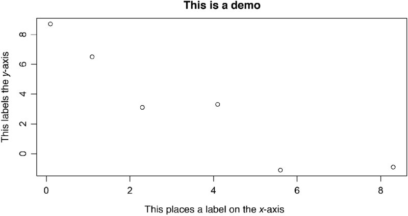
FIGURE 1.1 An example of a plot in R.
Some basic statistical analysis might involve inputting some values and performing some basic statistical analysis. Following the conventions already stated,
# this is a comment
x <- c(0.1,1.1,2.3,4.1, 5.6, 8.3) # create a vector of 6 values, these were just made up
y <- c(8.7, 6.5, 3.1, 3.3, −1.1, −0.9) #create a second vector
plot(x,y,xlab = “this places a label on the x axis”, ylab = “this labels the y axis”)
title(“this is a demo”)
# either “<-” or “=” can be used for assignments, but “<-” makes more sense.
# The reader should be aware that “=” and “<-” are not always interchangeable in R
(Figure 1.1).
The R code produces the data plotted in Figure 1.1.
[The commands for plots used in the book are simple commands that produce bitmap files that can easily be pasted into any report and resized. The actual graphs produced for the book use the slightly more complex tiff() function for better quality. For more information on better graphs check out help(tiff)].
Naming conventions used in this book:
| n | is always the sample size. |
| y | variants represent response variables. |
| noise | simulated white noise (independent normal random variables). |
| error | random error added to models (may not be white noise). |
| x | variants are independent/explanatory variables. |
| i | the square root of −1, in other words, we will not use this for any other purpose in this book. We will not use it as a variable or name. |
| time | usually integers from 1 to n, representing equally spaced time intervals. |
A number of simple statistical operations are worth mentioning, using the data simulated for Figure 1.1.
- mean(x) produces the output: 3.583333 which is the mean of the x values.
- sum(x) produces the output: 21.5 as expected (21.5/6 is the mean).
- var(y) produces the output: 15.28667, the sample variance of y.
Incidentally, it is best to write code in notepad or some other text editor and then paste it in R. As the code gets longer, this becomes mandatory (more sophisticated environments exist for writing and debugging R code, such as RStudio, but they are not necessary).
1.2 SPECIAL R CONVENTIONS
| Inf | infinity |
| NA | missing values |
| NaN | not a number, often an indeterminate form (Inf – Inf, 0/0, etc.) |
| TRUE | set a condition to true |
| FALSE | set a condition to false |
| == | Are two things equal? |
Examples
2==2 will produce the output: TRUE
2=2 will produce an error, as this is an attempt to assign a value to a number
2==3 will produce the output: FALSE
1/0 will produce the output: Inf
Inf/Inf will produce the output: NaN
1 - NA will produce the output: NA
1.3 COMMON STRUCTURES
All programming languages have some looping feature and some conditional action feature. In R, the “if” statement is used for conditional action and the “for” statement for iterating a process several times. These are not the only structures in R for this purpose, but they are all that is required for this book.
The “if” statement allows an action when a condition is met:
x <- 2        y <- 3        z <- 2        c <- TRUE        d <- TRUE
if(x == y) {c <- 1-c}
if(x == z) {d <- 1-d}
Can you guess what the values of c and d will be at the end? The variable c still has the value TRUE; it was unchanged, but d has the value 0, because it is 1—TRUE, which is 0 (see Exercise 1). TRUE can be understood as 1 and FALSE can be understood as 0 in R.
The “for” statement allows an action to occur a pre-set number of times. With mathematics, the “for” statement is often a summation or multiplication action.
Consider the formula ∑10j = 1j2 which can be evaluated in closed form m(m + 1)(2m + 1)/6, where m = 10, is 385.
sum <- 0
for(j in 1:10) {sum <- sum + j^2}
In the end, the sum will have the value 385. As with summation in most textbooks, as far as possible the letters j,k,l, and m will be used when indexing summation (i and n are already used as mentioned previously), although any letter could be used. For example,
sum <- 0
for(z in 1:10) {sum <- sum + z^2}
gets the right answer but would be considered poor style.
1.4 COMMON FUNCTIONS
| pi | is the value of pi, presumably to the decimal capacity of the computer. |
| sqrt() | the square root of a number. For example, sqrt(9) is 3. |
| log() | the (natural) logarithm of a number. For example, log(3) is slightly more than 1. |
| d^c | is the base d raised to the power c. For example, 2^4 is 16. |
| exp() | is exponentiation, the inverse of log(). For example, log(exp(5)) is 5. Also, exp(4) is about 2.718282^4 or about 54.6. |
| sin() | the sine function (all trigonometric functions assume radian inputs). |
| asin() | the arcsine or inverse sine function. For example, sin(asin(4)) = 4. |
| cos() | the cosine function. |
| acos() | the arccosine or inverse cosine function. |
| tan() | the tangent function. For example tan(3) is the same as sin(3)/cos(3). |
| atan() | the inverse tangent function. |
1.5 TIME SERIES FUNCTIONS
If what follows sounds like a foreign language, good, you are in the right class. Over the course of the book, these will all be introduced, but the students will learn to code primitive versions of these functions before they are allowed to use them.
| acf() | This function produces the autocorrelation plot and stores all information related to the autocorrelation function. |
| arima.sim() | This function simulates random noise with a user-specified correlation structure. |
| ar.yw() | This function produces all the information associated with Yule–Walker estimates for AR(m) processes. The related function ar.mle() will also be discussed. |
| spec.pgram() | This function produces a periodogram for a time series. |
| pacf() | This function produces the partial autocorrelation plot and stores all information related to the partial autocorrelation function. |
| ts() | This function defines a variable to be a time series. |
In some sense, a substantial portion of this course is to learn these functions, and all the background associated with these functions. Throughout the book, the underlying formulas will be derived and some crude R code that produces the computations and/or plots will be presented. Only when this is done does the student know exactly what the function does and is the student permitted to use the function, which can be viewed as elegant, often cosmetic, improvements over the crude R code.
1.6 IMPORTING DATA
Obviously, data sets are often very long and manual entry is unrealistic. The functions scan() and read.table() allow for reading large files. These will be discussed in Chapter 3 when the first time series data are read in and plotted.
Only scan() and read.table() are required for this book. However, read.csv() and read.delim() can be useful for reading formats that use commas or tabs to separate items. Using library(foreign), it is possible to import data from several other software formats (SPSS, Minitab, etc.).
The next chapter is a review of simple regression and an introduction to more R code in that context.
EXERCISES
-
Guess the output of the following bits of R code and check your answers (by typing the code in R).
(a) TRUE = FALSE; (b) TRUE == FALSE; (c) NA-NA; (d) 1/Inf; (e) Inf - Inf; (f) 1^Inf; (g) y <- 2, x <- 3, y == x; (h) 0/0; (i) 1 – TRUE; (j) 1 – FALSE; (k) TRUE + FALSE; (l) TRUE/FALSE; (m) 0^0.
-
Recall ∑mj = 1j = m(m + 1)/2. Write R code to find the sum ∑20j = 1j and verify that the sum is correct.
-
Write R code, using a “for” loop, to find the value 20! (20 factorial) and verify that it is correct.
-
Add log(15) + tan(π/2) in R.