
![]()
Input and Output
As a scripting language, R is perhaps not as flexible as Python or other languages, but as a statistical language, R provides all of the basic input and output capabilities that an average user is likely to need. In Chapter 3, you will learn how to get data into R and how to get output from R in the form and format you desire.
To prepare for our discussion of input and output, let me first remind you of some functions we have discussed and tell you about a few that we haven’t yet discussed. This will help greatly with your file management for both input and output.
Remember the functions getwd() and setwd() are used to identify and change the working directory. If the file is in the current directory, you can access it using only the file name. If you need a file in a different directory, you must give the path to the file as well as the name. If you want to know the information about a particular file, you can use the file.info() function. Sometimes, you might forget whether or not you saved a file to your working directory. You can find out whether you did by using the file.exists() function. As you have already seen, we can use ls() to get a list of all of the objects in the workspace and dir() to get a list of all of the files in the working directory. To get a complete list of all of the functions related to files and directories, just type ?files at the command prompt. Knowing these functions will make your life easier. Until you have memorized them, you may want to make a cheat sheet and keep it close at hand when you are programming.
You have already used the R console extensively to type in data and commands. When the demands of data input exceed the capacity of the console, you can access the R Editor for typing scripts (R code) and import worksheets to input data.
You also learned in Chapter 2 how to read in string data from a text file. In the example of the statistics quote, we made a simple replacement of one name with another. There are many more things you can do with strings, and we will discuss those in Chapter 15.
We can use the scan() function to read in data instead of typing the data in by using the c() function. For example, say we want to create a vector with 10 numbers. People are usually better at entering data in columns than rows. Here’s how to use scan() to build a vector:
> newVector <- scan ()
1: 11
2: 23
3: 44
4: 15
5: 67
6: 15
7: 12
8: 8
9: 9
10:
Read 9 items
> newVector
[1] 11 23 44 15 67 15 12 8 9
You simply type the numbers in one at a time and hit < Enter> when you are finished. It is also possible to read a vector into your workspace by using the scan function. Say you have a text file called “yvector.txt,” and have separated the numbers by spaces. Read it into the workspace as follows:
> yvector <- scan (" yvector . txt ", sep = " ")
Read 12 items
> yvector
[1] 11 22 18 32 39 42 73 27 34 32 19 15
In a similar way, we can get keyboard input using the readline() function. Examine the following code fragment so see how this works:
> myName <- readline (" What shall I call you ? ")
What shall I call you ? Larry
> myName
[1] " Larry "
3.1.1 The R Editor
Rstudio has some very convenient features in its graphical user interface. The Rstudio Editor is shown in Figure 3-1. You open this window by selecting from the menu bar the commands File ![]() New File
New File ![]() R script.
R script.
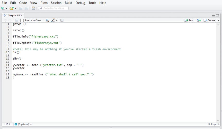
Figure 3-1. The Rstudio editor open
This is similar to a text processor; and many R programmers prefer to use different text editors. I find the Rstudio editor useful for writing lines of code and editing them before executing them. RStudio’s editor also includes a built-in debugger, which is very helpful in code development.
3.1.2 The R Data Editor
As you saw at the end of Chapter 1, the R Data Editor is a spreadsheet-like window into which you can type and edit data. To open the Data Editor, you must either already have a data frame, or you must create one. Although the Data Editor is not suitable for creating larger datasets, it is very good for quick changes to an existing dataset, as we discussed in Chapter 2. For example, suppose with our sports roster we needed to change Josh Smith’s Inches to 81. We might use the fix() function, which will allow us to click inside the variables replace ‘80’ with ‘81’. When you fix the labels, or make any other changes to the data frame, just close the R Data Editor to save the changes (see Figure 3-2).
> roster <- read.csv("roster.csv")
> fix(roster)
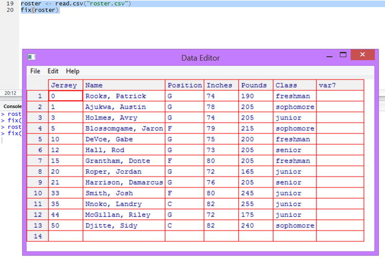
Figure 3-2. The Rstudio Data Editor open
3.1.3 Other Ways to Get Data Into R
We can read data into R from different kinds of files, including comma-separated value (CSV) files, text files, R data files, and others. The scan() function and the readline() function can be used as well.
You can also request user input via the console. Let’s examine these various approaches. We will discuss functional programming in more depth in Chapter 5, but as a teaser, see the following code to create a function that requests user input to calculate one’s body mass index (BMI):
BMI <- function () {
  cat (" Please enter your height in inches and weight in pounds :","
")
  height <- as.numeric ( readline (" height = "))
  weight <- as.numeric ( readline (" weight = "))
  bmi <- weight/(height^2)*703
  cat (" Your body mass index is:",bmi ,"
")
  if ( bmi < 18.5) risk = " Underweight "
  else if ( bmi >= 18.5 & bmi <= 24.9) risk = "Normal"
  else if ( bmi >= 25 & bmi <= 29.9) risk = "Overweight"
  else risk = "Obese"
  cat (" According to the National Heart, Lung, and Blood Institute,","
")
  cat (" your BMI is in the",risk ,"category.","
")
}
Open the R Editor and type the code just as you see it. Omit the R command prompts when typing code in the Editor window. To read the function into your R session, press <Ctrl> + A to select all the lines, and then press <Ctrl> + R to run the code. You should see the code in the R console now. When the function is executed, it will prompt the user for his or her height and weight. After the user enters these, the function then calculates and evaluates the person’s BMI. Because we provide the input from the keyboard, the function has no arguments, and we simply type BMI() and then press <Enter> to execute it. For example:
> BMI ()
Please enter your height in inches and weight in pounds :
height = 67
weight = 148
Your body mass index is: 23.17755
According to the National Heart, Lung, and Blood Institute,
your BMI is in the Normal category.
3.1.4 Reading Data from a File
The foreign and the Hmisc packages can read files produced by SPSS and many other programs (we’ve already met foreign). The basic operation in R to read in a data file is read.table. For text files, you must tell R if the first row of the dataset contains column headers that will be used as variable names. You must also tell read.table what your separator between variables is, that is, whether it is a tab, a space, or something else. If you use the read.csv function, it will assume that your data have a header row. You can control whether R converts strings to factors when it reads in the data by setting stringsAsFactors to TRUE or FALSE. The default behavior is TRUE. I usually set it to FALSE, because I do not necessarily want all strings to become factors. We will discuss factors in much more detail later.
Let’s see how these various input operations work in R. I’ve typed a brief history (from memory) of my recent cell phone purchases). We will read in the entire cellphone dataset from a tab-delimited text file called “cellphonetab.txt”. Remember that when the data are in text format, you must specify header = TRUE if you want to use the row of column headings in the first line. In this case, I want the strings to be recognized as factors, so I accept the default in this case by omitting stringsAsFactors = FALSE:
> cellPhones <- read.table ("cellphonetab.txt ", sep = "	", header = TRUE )
> str ( cellPhones )
'data.frame':    5 obs. of  2 variables:
 $ CellPhone: Factor w/ 5 levels "iPhone 4","iPhone 5",..: 4 5 1 2 3
 $ Year     : int  2006 2008 2010 2012 2014
3.1.5 Getting Data from the Web
It is also quite easy to download data from the web. For example, the Institute for Digital Research and Education at the University of California in Los Angeles has a series of tutorials on R with many example datasets (see Figure 3-3). Let’s download one of those lessons and work with it briefly.

Figure 3-3. The UCLA Institute for Digital Research and Education website
Although we have already discussed subsetting data, let’s go ahead and download the IDRE lesson and work with it briefly. See how easy it is to get the information from the website. We simply use the read.csv function with the URL to the data on the web as our source. Examine the following code snippet to see how the small dataset from IDRE can be used to help you learn subsetting:
> hsb2.small <- read.csv ("http://www.ats.ucla.edu/stat/data/hsb2_small.csv")
> names(hsb2.small)
[1] "id" "female" "race" "ses" "schtyp" "prog" "read" "write" "math" "science" "socst"
> (hsb3 <- hsb2.small [, c(1, 7, 8) ])
   id read write
1  70   57    52
2 121   68    59
3  86   44    33
4 141   63    44
5 172   47    52
6 113   44    52
##this data continues through 25 lines.
For example, you can learn how to subset the data by using comparison operators, such as selecting only the individuals with reading scores above or below a certain number. You can also combine the comparison operators so that you could select on multiple conditions. Here are all the variables, which makes it more obvious what the code above did. I learned the trick of enclosing a command in parentheses to print the result of the command from the IDRE lessons. The one command (hsb3 <- hsb2.small[, c(1, 7, 8)]) creates and prints the data frame hsb3, which contains the first, the seventh, and the eighth columns of hsb2.small, and prints the new data frame all in one statement. That’s efficiency at work:
> head (hsb2.small)
    id female race ses schtyp prog read write math science socst
1   70      0    4   1      1    1   57    52   41      47    57
2  121      1    4   2      1    3   68    59   53      63    61
3   86      0    4   3      1    1   44    33   54      58    31
4  141      0    4   3      1    3   63    44   47      53    56
5  172      0    4   2      1    2   47    52   57      53    61
6  113      0    4   2      1    2   44    52   51      63    61
3.2 R Output
R results appear by default in the R console or in the R graphics device, which we will examine in more detail in Chapter 10. We can also save output in different ways, for example, by writing data objects to files or saving graphics objects.
As you saw earlier with the example of the BMI function, You can use the cat() function, short for concatenate, to string together output to the console a line at a time. This is a very helpful way to print a combination of text and values. Note that you must use quotes and a backslash "n" to “escape” the new line character. If you want to enter a tab instead of a new line, use "t".
3.2.1 Saving Output to a File
The output analog of reading a file is writing it. In R, the basic operation is write.table. You can also use write.csv. When the data are to be saved in R format, you use the save command. Here is how to save the UCLA file data to a native R data file, which uses the extension .rda. You see that the new R data file is saved in the working directory. To read the file into R, instead of using read, you use load instead:
> save (hsb3, file = "hsb3save.rda")
> dir ()
 [1] "BeginningR.Rproj"                             "Chapter1.R"
 [3] "Chapter2.R"                                   "Chapter3.R"
 [5] "desktop.ini"                                  "fishersays.txt"
 [7] "GSS2012.sav"                                  "GSS2012merged_R5.sav"
 [9] "hsb3.RDS"                                     "hsb3save.rda"
[11] "Release Notes for the GSS 2012 Merged R5.pdf" "roster.csv"
[13] "stack.txt"                                    "yvector.txt"
> load ("hsb3save.rda")
> head (hsb3, 3)
   id read write
1  70   57    52
2 121   68    59
3  86   44    33
Let’s also save this data to a CSV file for practice. The following does the trick. We will also check to make sure the new file is in the working directory:
> write.csv( hsb3, file = "hsb3.csv")
> file.exists ("hsb3.csv")
[1] TRUE
Finally, we shall subject our poor hsb3 data to one last save, using a rather helpful set of commands saveRDS( ) and readRDS( ). Notice we take the object, save it as a file (it will show up in our working directory) and then we can read that file back in as a data object – notice we may even give it a new name as we read it back!
> saveRDS(hsb3, "hsb3.RDS")
> hsb3Copy <- readRDS("hsb3.RDS")