
Chapter 2
Starting Out: Becoming Familiar with R
What you will learn in this chapter:
- How to use R for simple math
- How to store results of calculations for future use
- How to create data objects from the keyboard, clipboard, or external data files
- How to see the objects that are ready for use
- How to look at the different types of data objects
- How to make different types of data objects
- How to save your work
- How to use previous commands in the history
So far you have learned how to obtain and install R, and how to bring up elements of the help system. As you have seen, R is a language and the majority of tasks require you to type commands directly into the input window. Like any language you need to learn a vocabulary of terms as well as the grammar that joins the words and makes sense of them. In this chapter you learn some of the basics that underpin the R language. You begin by using R as a simple calculator. Then you learn how to store the results of calculations for future use. In most cases, you will want to create and use complex data items, and you learn about the different kinds of data objects that R recognizes.
Some Simple Math
R can be used like a calculator and indeed one of its principal uses is to undertake complex mathematical and statistical calculations. R can perform simple calculations as well as more complex ones. This section deals with some of R’s commonly used mathematical functions. Learning how to carry out some of these simple operations will give you practice at using R and typing simple commands.
Use R Like a Calculator
You can think of R as a big calculator; it will perform many complicated calculations but generally, these are made up of smaller elements. To see how you can use R in this way, start by typing in some simple math:
> 3 + 9 + 12 -7
[1] 17
The first line shows what you typed: a few numbers with some simple addition and subtraction. The next line shows you the result (17). You also see that this line begins with [1] rather than the > cursor. R is telling you that the first element of the answer is 17. At the moment this does not seem very useful, but the usefulness becomes clearer later when the answers become longer. For the remainder of this book, the text will mimic R and display examples using the > cursor to indicate which lines are typed by the user; lines beginning with anything else are produced by R.
Now make the math a bit more complicated:
> 12 + 17/2 -3/4 * 2.5
[1] 18.625
To make sense of what was typed, R uses the standard rules and takes the multiplication and division parts first, and then does the additions and subtractions. If parentheses are used you can get a quite different result:
> (12 + 17/2 -3/4) * 2.5
[1] 49.375
Here R evaluates the part(s) in the parentheses first, taking the divisions before the addition and subtraction. Lastly, the result from the brackets is been multiplied by 2.5 to give the final result. It is important to remember this simple order when doing long calculations!
Many mathematical operations can be performed in R. In Table 2-1 you can see a few of the more useful mathematical operators.
Table 2-1: Some of the Mathematical Operations Available in R
| Command/Operation | Explanation |
| + - / * ( ) | Standard math characters to add, subtract, divide, and multiply, as well as parentheses. |
| pi | The value of pi (π), which is approximately 3.142. |
| x^y | The value of x is raised to the power of y, that is, xy. |
| sqrt(x) | The square root of x. |
| abs(x) | The absolute value of x. |
| factorial(x) | The factorial of x. |
| log(x, base = n) | The logarithm of x using base = n (natural log if none specified). |
| log10(x)log2(x) | Logarithms of x to the base of 10 or 2. |
| exp(x) | The exponent of x. |
| cos(x)sin(x)tan(x)acos(x)asin(x)atan(x) | Trigonometric functions for cosine, sine, tangent, arccosine, arcsine, and arctangent, respectively. In radians. |
Some of the mathematical operators can be typed in by themselves—for example, + - * ^ but others require one or more additional instructions. The log() command, for example, requires one or two instructions, the first being the number you want to evaluate and the second being the base of the log you require. If you type in only a single instruction, R assumes that you require the natural log of the value you specified. In the following activity you have the opportunity to try out some of the math and gain a feel for typing commands into the R console window.
> pi * 2^3 – sqrt(4)> abs(12-17*2/3-9)> factorial(4)> log(2, 10)
> log(2, base = 10)
> log10(2)> log(2)> exp(0.6931472)> log10(2)> 10^0.30103> sin(45 * pi / 180)asin(0.7071068) * 180 / piNow that you have the idea about using some simple math you need to look at how you can store the results of calculations for later use.
Storing the Results of Calculations
Once you have performed a calculation you can save the result for use in some later calculation. The way to do this is to give the result a name. R uses named objects extensively and understanding these objects is vital to working with R. To make a result object you simply type a name followed by an equals sign, and then anything after the = will be evaluated and stored as your result. The formula should look like this:
object.name = mathematical.expressionThe following example makes a simple result object from some mathematical expressions; the result can be recalled later:
> ans1 = 23 + 14/2 - 18 + (7 * pi/2)Here R is instructed to create an item called ans1 and to make this from the result of the calculation that follows the = sign. Note that if you carry out this command you will not see a result. You are telling R to create the item from the calculation but not to display it. To get the result you simply type the name of the item you just created:
> ans1
[1] 22.99557
You can create as many items as you like (although eventually you would fill up the memory of your computer); here is another example:
> ans2 = 13 + 11 + (17 - 4/7)Now you have two results, ans1 and ans2. You can use these like any other value in further calculations. For example:
> ans1 + ans2 / 2
[1] 43.20986
> ans3 = ans2 + 9 - 2 + pi
In these examples the = sign is used. This is perfectly logical but R allows you an alternative. In older versions of R and in most of the help examples you will see that the = sign is rarely used and a sort of arrow is used instead. For example:
> ans4 <- 3 + 5
> ans5 <- ans1 * ans2
Here two new result objects are created (ans4 and ans5) from the expressions to the right of the “arrow.” This is more flexible than the = sign because you can reverse the direction of the arrow:
> ans3 + pi / ans4 -> ans6If the regular = sign was used instead in this example, you would get an error.
The results you have created so far are simple values that have resulted from various mathematical operations. These result objects are revisited later in the chapter. The “Making Named Objects” section provides a look at listing the objects created as well as some rules for object names. Most often you will have sets of data to examine; these will comprise more complicated sets of numbers. Being able to create more complex data is covered in the next section.
Reading and Getting Data into R
So far you have looked at some simple math. More often you will have sets of data to examine (that is, samples) and will want to create more complex series of numbers to work on. You cannot perform any analyses if you do not have any data so getting data into R is a very important task. This next section focuses on ways to create these complex samples and get data into R, where you are able to undertake further analyses.
Using the combine Command for Making Data
The simplest way to create a sample is to use the c() command. You can think of this as short for combine or concatenate, which is essentially what it does. The command takes the following form:
c(item.1, item.2, item.3, item.n)Everything in the parentheses is joined up to make a single item. More usually you will assign the joined-up items to a named object:
sample.name = c(item.1, item.2, item.3, item.n)This is much like you did when making simple result objects, except now your sample objects consist of several bits rather than a single value.
Entering Numerical Items as Data
Numerical data do not need any special treatment; you simply type the values, separated by commas, into the c() command.
In the following example, imagine that you have collected some data (a sample) and now want to get the values into R:
>data1 = c(3, 5, 7, 5, 3, 2, 6, 8, 5, 6, 9)Now just create a new object to hold your data and then type the values into the parentheses. The values are separated using commas.
The “result” is not automatically displayed; to see the data you must type its name:
> data1
 [1] 3 5 7 5 3 2 6 8 5 6 9
Previously the named objects contained single values (the result of some mathematical calculation). Here the named object data1 contains several values, forming a sample. The [1] at the beginning shows you that the line begins with the first item (the number 3). When you get larger samples and more values, the display may well take up more than one line of the display, and R provides a number at the beginning of each row so you can see “how far along” you are. In the following example you can see that there are 41 values in the sample:
 [1]  582  132  716  515  158   80  757  529  335  497 3369  746  201  277  593
[16]  361  905 1513  744  507  622  347  244  116  463  453  751  540 1950  520
[31]  179  624  448  844 1233  176  308  299  531   71  717
The second row starts with [16], which tells you that the first value in that row is the 16th in the sample. This simple index system makes it a bit easier to pick out specific items.
You can incorporate existing data objects with values to make new ones simply by incorporating them as if they were values themselves (which of course they are). In this example you take the numerical sample that you made earlier and incorporate it into a larger sample:
> data1
 [1] 3 5 7 5 3 2 6 8 5 6 9
> data2 = c(data1, 4, 5, 7, 3, 4)
> data2
 [1] 3 5 7 5 3 2 6 8 5 6 9 4 5 7 3 4
Here you take your first data1 object and add some extra values to create a new (larger) sample. In this case you create a new item called data2, but you can overwrite the original as part of the process:
> data1 = c(6, 7, 6, 4, 8, data1)
> data1
 [1] 6 7 6 4 8 3 5 7 5 3 2 6 8 5 6 9
Now adding extra values at the beginning has modified the original sample.
Entering Text Items as Data
If the data you require are not numerical, you simply use quotes to differentiate them from numbers. There is no difference between using single and double quotes; R converts them all to double. You can use either or both as long as the surrounding quotes for any single item match, as shown in the following:
our.text = c(“item1”, “item2”, ‘item3’)In practice though, it is a good habit to stick to one sort of quote; single quote marks are easier to type.
The following example shows a simple text sample comprising of days of the week:
> day1 = c('Mon', 'Tue', 'Wed', 'Thu')
> day1
[1] "Mon" "Tue" "Wed" "Thu"
You can combine other text objects in the same way as you did for the numeric objects previously, like so:
> day1 = c(day1, 'Fri')
> day1
[1] "Mon" "Tue" "Wed" "Thu" "Fri"
If you mix text and numbers, the entire data object becomes a text variable and the numbers are converted to text, shown in the following. You can see that the items are text because R encloses each item in quotes:
> mix = c(data1, day1)
> mix
 [1] "3"   "5"   "7"   "5"   "3"   "2"   "6"   "8"   "5"   "6"   "9"   "Mon"
[13] "Tue" "Wed" "Thu" "Fri"
The c() command used in the previous example is a quick way of getting a series of values stored in a data object. This command is useful when you don’t have very large samples, but it can be a bit tedious when a lot of typing is involved. Other methods of getting data into R exist, which are examined in the next section.
Using the scan Command for Making Data
When using the c() command, typing all those commas to separate the values can be a bit tedious. You can use another command, scan(), to do a similar job. Unlike the c() command you do not insert the values in the parentheses but use empty parentheses. The command then prompts you to enter your data. You generally begin by assigning a name to hold the resulting data like so:
our.data = scan()Once you press the Enter key you will be prompted to enter your data. The following activity illustrates this process.
> data3 = scan()1: 6 7 8 7 6 3 8 9 10 711: 6 913: 13:
Read 12 items> data3
[1] 6 7 8 7 6 3 8 9 10 7 6 9Entering Text as Data
You can enter text using the scan() command, but if you simply enter your items in quotes you will get an error message. You need to modify the command slightly like so:
scan(what = 'character')You must tell R to expect that the items typed in are characters, not numbers; to do this you add the what = ‘character’ part in the parentheses. Note that character is in quotes. Once the command runs it operates in an identical manner as before.
In the following example a simple data item is created containing text stating the days of the week:
> day2 = scan(what = 'character')
1: Mon Tue Wed
4: Thu
5:
Read 4 itemsNote that quotes are not needed for the entered data. R is expecting the entered data to be text so the quotes can be left out. Typing the name of the object you just created displays the data, and you can see that they are indeed text items and the quotes are there:
> day2
[1] "Mon" "Tue" "Wed" "Thu"Using the Clipboard to Make Data
The scan() command is easier to use than the c() command because it does not require commas. The command can also be used in conjunction with the clipboard, which is quite useful for entering data from other programs (for example, a spreadsheet). To use these commands, perform the following steps:
If the data are text, you add the what = ‘character’ instruction to the scan() command as before.
At this point, if you can open the file in a spreadsheet, proceed with the aforementioned four steps. If the file opens in a text editor or word processor, you must look to see how the data items are separated before continuing.
If the data are separated with simple spaces, you can simply copy and paste. If the data are separated with some other character, you need to tell R which character is used as the separator. For example, a common file type is CSV (comma-separated values), which uses commas to separate the data items. To tell R you are using this separator, simply add an extra part to your command like so:
scan(sep = ‘,’)In this example R is told to expect a comma; note that you need to enclose the separator in quotes. Here are some comma-separated numerical data:
23,17,12.5,11,17,12,14.5,9
11,9,12.5,14.5,17,8,21To get these into R, use the scan() command like so:
> data4 = scan(sep = ',')
1: 23,17,12.5,11,17,12,14.5,9
9: 11,9,12.5,14.5,17,8,21
16:
Read 15 items
> data4
[1] 23.0 17.0 12.5 11.0 17.0 12.0 14.5 9.0 11.0 9.0 12.5 14.5 17.0 8.0 21.0Note that you have to press the Enter key to finish the data entry. Note also that some of the original data had decimal points (for example, 14.5); R appends decimals to all the data so that they all have the same level of precision. If your data are separated by tab stops you can use “ ” to tell R that this is the case.
If the data are text, you simply add what = ‘character’ and proceed as before. Here are some text data contained in a CSV text file:
"Jan","Feb","Mar","Apr","May","Jun"
"Jul","Aug","Sep","Oct","Nov","Dec"To get these data entered into R, perform the following steps:
The set of operations appears as follows:
> data5 = scan(sep = ',', what = 'char')
1: "Jan","Feb","Mar","Apr","May","Jun"
7: "Jul","Aug","Sep","Oct","Nov","Dec"
13:
Read 12 items
> data5
[1] "Jan" "Feb" "Mar" "Apr" "May" "Jun" "Jul" "Aug" "Sep" "Oct" "Nov" "Dec"In this example both sep = and what = instructions are used. Additionally, the scan() command allows you to create data items from the keyboard or from clipboard entries, thus enabling you to move data from other applications quite easily. It is also possible to get the scan() command to read a file directly as described in the following section.
Reading a File of Data from a Disk
To read a file with the scan() command you simply add file = ‘filename’ to the command. For example:
> data6 = scan(file = 'test data.txt')
Read 15 items
> data6
[1] 23.0 17.0 12.5 11.0 17.0 12.0 14.5 9.0 11.0 9.0 12.5 14.5 17.0 8.0 21.0In this example the data file is called test data.txt, which is plain text, and the numerical values are separated by spaces. Note that the filename must be enclosed in quotes (single or double). Of course you can use the what = and sep = instructions as appropriate.
R looks for your data file in the default directory. You can find the default directory by using the getwd() command like so:
> getwd()
[1] "C:/Documents and Settings/Administrator/My Documents"
> getwd()
[1] "/Users/markgardener"
> getwd()
[1] "/home/mark"The first example shows the default for a Windows XP machine, the second example is for a Macintosh OS X system, and the final example is for Linux (Ubuntu 10.10).
If your file is somewhere else you must type its name and location in full. The location is relative to the default directory; in the preceding example the file was on the desktop so the command ought to have been:
> data6 = scan(file = 'Desktop/test data.txt')The filename and directories are all case sensitive. You can also type in a URL and link to a file over the Internet directly; once again the full URL is required.
It may be easier to point permanently at a directory so that the files can be loaded simply by typing their names. You can alter the working directory using the setwd() command:
setwd('pathname')When using this command, replace the pathname part with the location of your target directory. The location is always relative to the current working directory, so to set to my Desktop I used the following:
> setwd('Desktop')
> getwd()
[1] "/Users/markgardener/Desktop"To step up one level you can type the following:
setwd('..')You can look at a directory and see which files/folders are within it using the dir() or list.files() command:
dir()
list.files()The default is to show the files and folders in the current working directory, but you can type in a path (in single quote marks) to list files in any directory. For example:
dir('Desktop')
dir('Documents')
dir('Documents/Excel files')Note that the listing is in alphabetical order; files are shown with their extensions and folders simply display the name. If you have files that do not have extensions (for example: .txt, .doc), it is harder to work out which are folders and which are files. Invisible files are not shown by default, but you can choose to see them by adding an extra instruction to the command like so:
dir(all.files = TRUE)In Windows and Macintosh OS there is an alternative method that enables you to select a file. You can include the instruction file.choose() as part of your scan() command. This opens a browser-type window where you can navigate to and select the file you want to read:
> data7 = scan(file.choose())
Read 15 items
> data7
[1] 23.0 17.0 12.5 11.0 17.0 12.0 14.5 9.0 11.0 9.0 12.5 14.5 17.0 8.0 21.0In the preceding example the target file was a plain text file with numerical data separated by spaces. If you have text or the items are separated by other characters, you use the what = and sep = instructions as appropriate, like so:
> data8 = scan(file.choose(), what = 'char', sep = ',')
Read 12 items
> data8
[1] "Jan" "Feb" "Mar" "Apr" "May" "Jun" "Jul" "Aug" "Sep" "Oct" "Nov" "Dec"In this example, the target file contained the month data that you met previously; the file was a CSV file where the names of the months (text labels) were separated with commas.
The file.choose() instruction is useful because you can select files from different directories without having to alter the working directory or type the names in full.
So far the data items that you have created are simple; they contain either a single value (the result of a mathematical calculation) or several items. A list of data items is called a vector. If you only have a single value, your vector contains only one item, that is, it has a length of 1. If you have multiple values, your vector is longer. When you display the list R provides an index to help you see how many items there are and how far along any particular item is. Think of a vector as a one-dimensional data object; most of the time you will deal with larger datasets than single vectors of values.
Reading Bigger Data Files
The scan() command is helpful to read a simple vector. More often though, you will have complicated data files that contain multiple items (in other words two-dimensional items containing both rows and columns). Although it is possible to enter large amounts of data directly into R, it is more likely that you will have your data stored in a spreadsheet. When you are sent data items, the spreadsheet is also the most likely format you will receive. R provides the means to read data that is stored in a range of text formats, all of which the spreadsheet is able to create.
The read.csv() Command
In most cases you will have prepared data in a spreadsheet. Your dataset could be quite large and it would be tedious to use the clipboard. When you have more complex data it is better to use a new command—read.csv():
read.csv()As you might expect, this looks for a CSV file and reads the enclosed data into R. You can add a variety of additional instructions to the command. For example:
read.csv(file, sep = ',', header = TRUE, row.names)You can replace the file with any filename as before. By default the separator is set to a comma but you can alter this if you need to. This command expects the data to be in columns, and for each column to have a helpful name. The instruction header = TRUE, the default, reads the first row of the CSV file and sets this as a name for each column. You can override this with header = FALSE. The row.names part allows you to specify row names for the data; generally this will be a column in the dataset (the first one is most usual and sensible). You can set the row names to be one of the columns by setting row.names = n, where n is the column number.
Some simple example data are shown in Table 2-2. Here you can see two columns; each one is a variable. The first column is labeled abund; this is the abundance of some water-living organism. The second column is labeled flow and represents the flow of water where the organism was found.
Table 2-2: Simple Data From a Two Column Spreadsheet
| abund | flow |
| 9 | 2 |
| 25 | 3 |
| 15 | 5 |
| 2 | 9 |
| 14 | 14 |
| 25 | 24 |
| 24 | 29 |
| 47 | 34 |
In this case there are only two columns and it would not take too long to use the scan() command to transfer the data into R. However, it makes sense to keep the two columns together and import them to R as a single entity. To do so, perform the following steps:
> fw = read.csv(file.choose())> fw
abund flow
1 9 2
2 25 3
3 15 5
4 2 9
5 14 14
6 25 24
7 24 29
8 47 34In the general, the read.csv() command is pretty useful because the CSV format is most easily produced by a wide variety of computer programs, spreadsheets, and is eminently portable. Using CSV means that you have fewer options to type into R and consequently less typing.
Alternative Commands for Reading Data in R
There are many other formats besides CSV in which data can exist and in which other characters, including spaces and tabs, can separate data. Consequently, the read.table() command is actually the basic R command for reading data. It enables you to read most formats of plain-text data. However, R provides variants of the command with certain defaults to make it easier when specifying some common data formats, like read.csv() for CSV files. Since most data is CSV though, the read.csv()is the most useful of these variants. But you may run into alternative formats, and the following list outlines the basic read.table() as well as other commands you can use to read various types of data:
- In the following example the data are separated by simple spaces. The read.table() command is a more generalized command and you could use this at any time to read your data. In this case you have to specify the additional instructions explicitly. The defaults are set to header = FALSE, sep = “ “ (a single space), and dec = “.”, for example.
data1 data2 data3 1 2 4 4 5 3 3 4 5 3 6 6 4 5 9 > my.ssv = read.table(file.choose(), header = TRUE) > my.ssv = read.csv(file.choose(), sep = ' ') - The next example shows data separated by tabs. If you have tab-separated values you can use the read.delim() command. In this command R assumes that you still have column heading names but this time the separator instruction is set to sep = “ ” (a tab character) by default:
data1 data2 data3 1 2 4 4 5 3 3 4 5 3 6 6 4 5 9 > my.tsv = read.delim(file.choose()) > my.tsv = read.csv(file.choose(), sep = ' ') > my.tsv = read.table(file.choose(), header = TRUE, sep = ' ') - The next example also shows data separated by tabs. In some countries the decimal point character is not a period but a comma, and a semicolon often separates data values. If you have a file like this you can use another variant, read.csv2(). Here the defaults are set to sep = “;”, header = TRUE, and dec = “,”.
day data1 data2 data3 mon 1 2 4 tue 4 5 3 wed 3 4 5 thu 3 6 6 fri 4 5 9 > my.list = read.delim(file.choose(), row.names = 1) > my.list = read.csv(file.choose(), row.names = 1, sep = ' ') > my.list = read.table(file.choose(), row.names = 1, header = TRUE, sep = ' ')
These commands essentially all perform the same function; the differences lie in the defaults. Regardless of which method you choose, getting data into R is a fundamental operation; you cannot do anything without having the data first. Bear the following checklist in mind when looking to get data from disk:
Missing Values in Data Files
In the examples you have seen so far the samples in the data files have all been the same length. In the real world samples are often of unequal size. The following example contains two samples, one called mow and one called unmow. The mow sample contains five values, whereas the unmow sample contains only four values. When these data are read into R from a spreadsheet or text file, the program recognizes that you have multiple columns of data and sets them out accordingly. R makes your data into a neat rectangular item and fills in any gaps with NA.
In the following example the data were stored in a CSV file and were read into R with the read.csv() command:
> grass = read.csv(file.choose())
> grass
mow unmow
1 12 8
2 15 9
3 17 7
4 11 9
5 15 NAHere the data have been called grass and you can see that R has filled in the gap using NA. R always pads out the shorter samples using NA to produce a rectangular object. This is called a data frame. The data frame is an important kind of R object because it is used so often in statistical data manipulation and is how you generally have data in spreadsheets.
Although the NA can be dealt with fairly easily you should strive to create data frames that do not contain them if at all possible. In the following example the data have been rearranged. There are still two columns, but the first contains all the values and the second contains a name that relates to one of the previous column headings:
species cut
1 12 mow
2 15 mow
3 17 mow
4 11 mow
5 15 mow
6 8 unmow
7 9 unmow
8 7 unmow
9 9 unmowYou can see that the label in the second column corresponds to a value in the first column. The first five items relate to the previous mow sample and the next four belong to the unmow sample. In statistical parlance the species column is called the response variable and the cut column is the predictor variable (or predictor factor).
R recognizes NA as a special kind of data object. It is important to know when your data contains NA items and what to do when you encounter them.
Viewing Named Objects
So far you have seen examples of creating data objects from some simple math and from reading in data files. In a general way you “make” new items by providing a name followed by the instruction that creates it. R is object oriented, which means that it expects to find named things to deal with in some way. For example, if you are conducting an experiment and collecting data from several samples, you want to create several named data objects in R in order to work on them and do your analyses later on.
As a reminder, the following examples show a few of the different ways you have seen thus far to create named items:
answer1 = 23 + 17/2 + pi/4
my.data = read.csv(file.choose())
sample1 = c(2, 5, 7, 3, 9, 4, 5)Now it is time to learn how to view these items in R and remove them as necessary. The following sections cover these topics.
Viewing Previously Loaded Named-Objects
Once you have made a few objects and have them stored in R, you might forget what you have previously loaded as time goes on. You need a way to see what R objects are available; to do this you use the ls() command like so:
ls()Viewing All Objects
The ls() command lists all the named items that you have available. You can also use the objects() command; (this is identical in function but slightly longer to type!) The result of either command is to list the objects stored in R at the current moment:
> ls()
[1] "answer1" "my.data" "sample1"This example contains three objects. The objects are listed in alphabetical order (with all the uppercase before the lowercase); if you have a lot of objects, the display will run to more lines like so:
[1] "A" "A.r" "B" "CI"
[5] "CI.1" "CI.dn" "CI.up" "Ell.F"
[9] "F" "F1" "area" "az"
[13] "bare" "beetle.cca" "beta" "bf"
[17] "bf.beta" "bf.lm" "biol" "biol.cca"
[21] "biomass" "bird" "bp" "bs"
[25] "bss" "but" "but.lm" "c3" Here there are 28 objects. At the beginning of each new row the display shows you an index number relating to “how far along” the list of items you are. For example the bare data object is the 13th item along (alphabetically). If you do not have any named objects at all, you get the following “result”:
> ls()
character(0)Viewing Only Matching Names
You may want to limit the display to objects with certain names; this is especially helpful if you have a lot of data already in R. You can limit the display by giving R a search pattern to match. For example:
> ls(pattern = 'b')
[1] "bare" "beetle.cca" "beta" "bf" "bf.beta"
[6] "bf.lm" "biol" "biol.cca" "biomass" "bird"
[11] "bp" "bs" "bss" "but" "but.lm"
[16] "cbh" "cbh.glm" "cbh.sf" "food.b" "nectar.b"
[21] "pred.prob" "prob2odd" "tab.est" "tab1" "tab2"Here the pattern looks for everything containing a “b”. This is pretty broad so you can refine it by adding more characters:
> ls(pattern = 'be')
[1] "beetle.cca" "beta" "bf.beta" Now the pattern picks up objects with “be” in the name. If you want to search for objects beginning with a certain letter you use the ^ character like so:
> ls(pattern = '^b')
[1] "bare" "beetle.cca" "beta" "bf" "bf.beta"
[6] "bf.lm" "biol" "biol.cca" "biomass" "bird"
[11] "bp" "bs" "bss" "but" "but.lm"Compare the following search listings. In the first case the pattern matches objects beginning with “be” but in the second case the letters are enclosed in square brackets:
> ls(pattern = '^be')
[1] "beetle.cca" "beta"
> ls(pattern = '^[be]')
[1] "bare" "beetle.cca" "beta" "bf" "bf.beta"
[6] "bf.lm" "biol" "biol.cca" "biomass" "bird"
[11] "bp" "bs" "bss" "but" "but.lm"
[16] "eF" "eF2" "env"The effect of the square brackets is to isolate the letters; each is treated as a separate item, hence objects beginning with “b” or “e” are matched. You can receive the same result using a slightly different approach as well:
ls(pattern = '^b|^e')The vertical brace (sometimes called a pipe) character stands for or, that is, you want to search for objects beginning with “b” or beginning with “e”.
To find objects ending with a specific character you use a dollar sign at the end like so:
> ls(pattern = 'm$')
[1] "bf.lm" "but.lm" "cbh.glm" "dep.pm"
[5] "dm" "frit.glm" "frit.lm" "frit.sum"
[9] "hlm" "mf.lm" "mr.lm" "n.glm"
[13] "newt.glm" "newt.test.glm" "sales.lm" "sm"
[17] "t.glm" "test.glm" "test.lm" "test1.glm"
[21] "tt.glm" "worm.pm"You can use the period as a wildcard and R will match any character:
> ls(pattern = 'a.e')
[1] "area" "bare" "date" "sales" "sales.frame"
[6] "sales.lm" "sales.ts" "water"
> ls(pattern = 'a..e')
[1] "tab.est" "treatment"In the first example a single wildcard was used but in the second there are two. This pattern matching uses more or less the same conventions as standard Regular Expressions, which are found in many programs. The ones demonstrated here are only a few of the array of options available. You can use help(regex) in R to see much more detail.
Removing Objects from R
You can remove objects from memory and therefore permanently delete them using the rm() or remove() commands. To remove objects you can simply list them in the parentheses of the command:
rm(list)
remove(list)You can type the names of the objects separated by commas. For example:
>rm(answer1, my.data, sample1)This removes the objects answer1, my.data, and sample1 from the workspace. You can use the ls() command to produce a list, which will then be deleted. You need to include the instruction list in the command like so:
>rm(list = ls(pattern = '^b'))Here the ls() command is used to search for objects beginning with “b” and remove them.
rm(list = ls())Types of Data Items
So far you have seen how to create some simple mathematical results, how to create simple samples, and how to read in more complex data containing multiple columns. Now is a good time to look at the types of data items that you may come across. Your data items can exist in one of two forms: numbers or text values. R regards these as numeric or character.
Number Data
Plain values that are whole numbers are integer values, whereas values that contain decimals are numeric. The distinction is fairly minor, but if you have a list of values that contain both integers and decimals, R will regard the entire sample as numeric.
> data3
 [1]  6  7  8  7  6  3  8  9 10  7  6  9
> data7
[1] 23.0 17.0 12.5 11.0 17.0 12.0 14.5 9.0 11.0 9.0 12.5 14.5 17.0 8.0 21.0In the first example the values are all whole numbers. In the second example some of them have decimal places, but R appends decimals to all of the data to achieve an equal level of precision; in this case they all have at least one decimal place.
Text Items
If you do not have numbers, you must have text. R recognizes two sorts of text data items. You can think of the first kind as plain text labels; R calls these character values.
> data8
[1] "Jan" "Feb" "Mar" "Apr" "May" "Jun" "Jul" "Aug" "Sep" "Oct" "Nov" "Dec"These items display as plain text and have the quote marks to remind you. However, another type of non-numeric data is called a factor:
> cut
[1] mow mow mow mow mow unmow unmow unmow unmow
Levels: mow unmowHere the data are text but they are not in quotes. When they are displayed the text appears plain without quote marks, but with an additional line showing you how many different things there are in this list. Recall the data that you met previously:
> grass
  species   cut
1      12   mow
2      15   mow
3      17   mow
4      11   mow
5      15   mow
6       8 unmow
7       9 unmow
8       7 unmow
9 9 unmowWhen R reads the data from the data file it assumes that the text column corresponds to the numeric column and sets the text to a factor rather than as a character. In most instances this is what you want for statistical analyses. However, you can elect to read any column as plain text using the as.is = instruction. To do this for the previous mowing data, for example, you would type:
grass2 = read.csv(file.choose(), as.is = 2)Here you tell R that the second column in your data file is to be regarded as plain text rather than a factor.
Converting Between Number and Text Data
You can shift between the two kinds of text quite easily. The following example begins with data that is a factor. The as.character() command is used to convert to plain text. Then the plain text is converted back to a factor using the as.factor() command:
> cut
[1] mow mow mow mow mow unmow unmow unmow unmow
Levels: mow unmow
> cut2 = as.character(cut)
> cut2
[1] "mow" "mow" "mow" "mow" "mow" "unmow" "unmow" "unmow" "unmow"
> cut3 = as.factor(cut2)
> cut3
[1] mow mow mow mow mow unmow unmow unmow unmow
Levels: mow unmowIn this case new data objects were created but the original object could be overwritten with the new one.
You can do a similar thing with numbers. If you begin with data that contain decimals, that is, numeric, you can convert to integers using the as.integer() command. You can convert integer values to numeric using the as.numeric() command:
> data7
[1] 23.0 17.0 12.5 11.0 17.0 12.0 14.5 9.0 11.0 9.0 12.5 14.5 17.0 8.0 21.0
> data7i = as.integer(data7)
> data7i
[1] 23 17 12 11 17 12 14 9 11 9 12 14 17 8 21
> data7n = as.numeric(data7i)
> data7n
[1] 23 17 12 11 17 12 14 9 11 9 12 14 17 8 21You can also convert numbers to text using as.character():
> data7c = as.character(data7)
> data7c
[1] "23" "17" "12.5" "11" "17" "12" "14.5" "9" "11" "9" "12.5"
[12] "14.5" "17" "8" "21"You can also try converting text into numbers like so:
> data7nt = as.numeric(data7c)
> data7nt
[1] 23.0 17.0 12.5 11.0 17.0 12.0 14.5 9.0 11.0 9.0 12.5 14.5 17.0 8.0 21.0This works out fine if the text is sensible; in the preceding example the text values were originally numbers. Now see what happens if you try this on a factor:
> cut
[1] mow mow mow mow mow unmow unmow unmow unmow
> cut.n = as.numeric(cut)
> cut.n
[1] 1 1 1 1 1 2 2 2 2Here you get a surprising (but potentially useful) result; the numbers relate directly to the different factors that you have. If you try to convert something that really is not going to work, R gives a warning like so:
> data8
 [1] "Jan" "Feb" "Mar" "Apr" "May" "Jun" "Jul" "Aug" "Sep" "Oct" "Nov" "Dec"
> data8n = as.numeric(data8)
Warning message:
NAs introduced by coercion
> data8n
[1] NA NA NA NA NA NA NA NA NA NA NA NAIn this case the data is plain text and cannot be forced into any sensible number, so you end up with a string of NAs. If you were to convert the plain text to a factor first and then to a number, that would be a different story:
> data8c = as.numeric(as.factor(data8))
> data8c
[1] 5 4 8 1 9 7 6 2 12 11 10 3Here one command is nested inside the other. R evaluated the as.factor() part first and then converted that into numbers. You started with twelve months and can see that they have been assigned numbers; notice how R has indexed them alphabetically.
The Structure of Data Items
The data that you have can exist in a variety of forms (or structures). For example, you may have many individual samples, each item being a separate entity. On the other hand, you may have complicated data—the results of surveys, for example—that each contain several columns of values. R recognizes several forms of data and these forms each have their own particular uses. This section focuses on these different forms of data.
Your data can exist as numerical or character data as you saw in the previous section. However, these data items can also be constructed and put together in a variety of ways. This section looks at these different structures: vector, matrix, data frame, and list.
Vector Items
So far you have met two kinds of data: vectors and data frames. A vector can be thought of as a one-dimensional object. You created vectors containing a single item from some mathematical operations; you also created vectors by making simple samples of values and text. Here are two simple vectors:
> data8
[1] "Jan" "Feb" "Mar" "Apr" "May" "Jun" "Jul" "Aug" "Sep" "Oct" "Nov" "Dec"
> data7
[1] 23.0 17.0 12.5 11.0 17.0 12.0 14.5 9.0 11.0 9.0 12.5 14.5 17.0 8.0 21.0The first one is a vector of text values; the second is a vector of numeric values. You could also have a vector of factors—the cut object from earlier is an example of a factor vector:
> cut
[1] mow   mow   mow   mow   mow   unmow unmow unmow unmow
Levels: mow unmowData Frames
You have also already met the data frame. A data frame is a two-dimensional object, that is, it has rows and columns. R treats the columns as separate samples or variables, and the rows represent the replicates or observations. All data frames are rectangular and R will pad out any “short” columns using NA.
Here is a simple example that you met previously. There are two columns; one represents a sample called mow and contains five replicates/observations. The second column is called unmow and contains four observations:
> grass
mow unmow
1 12 8
2 15 9
3 17 7
4 11 9
5 15 NAEach column can be a separate type of data; in the following example the data are reorganized so that the first is numeric and the second is a factor:
> grass
  species   cut
1      12   mow
2      15   mow
3      17   mow
4      11   mow
5      15   mow
6       8 unmow
7       9 unmow
8       7 unmow
9 9 unmowThe second form of the data frame is most useful, especially for statistical analyses. This is because there are no NA items.
Matrix Objects
A matrix is a two-dimensional data object. At first glance a matrix looks just like a data frame:
> bird
               Garden Hedgerow Parkland Pasture Woodland
Blackbird          47       10       40       2        2
Chaffinch          19        3        5       0        2
Great Tit          50        0       10       7        0
House Sparrow      46       16        8       4        0
Robin               9        3        0       0        2
Song Thrush         4        0        6       0        0
In this example you can see some observations of a variety of common birds and the habitat in which they were observed. The matrix has rows and columns just like a data frame but the object is handled differently, and some commands require a matrix to operate on rather than a data frame. Unlike a data frame, a matrix cannot contain mixed data; all the columns must be the same type, that is, all numeric or all character. A matrix can consist of a single row or a single column and so can also appear just like a vector object. You learn how to tell which is which shortly.
List Objects
A list is a series of items bundled together to form a single object. In the following example the grass data you met previously has been made into a list:
> grass.l
$mow
[1] 12 15 17 11 15

$unmow
[1] 8 9 7 9
When you look at it you see each vector listed separately along with its name, which is prefixed with a dollar sign. This example list is very simple and contains only two vectors. A list could be constructed from objects of various sorts, and you might have, for example, a matrix, a data frame, and several vectors containing a mixture of numbers and characters. The list is a flexible object but also harder to deal with, as you will find out in due course.
Examining Data Structure
As you collect and work on new data you will inevitably build a collection of items. Different kinds of analysis will require different approaches, and you will need to examine a data object in order to work out what kind it is so that you can determine the best strategy for dealing with it.
The vector is the smallest unit in the data structure. When you start to bundle vectors together you make more complex items. The complex item you make can be a data frame, a matrix, or a list.
You need a way to tell which form your data are in. If you look at a particular object, you can get a clue; a simple vector will be a one-dimensional set of characters or numbers. A data frame or a matrix will have a rectangular two-dimensional structure. A list will appear as a series of separately named vectors; each name starts with a dollar sign ($). The difficulty is differentiating between the matrix and the data frame. You can use the str() command to examine the structure of an object like so:
> str(grass)
'data.frame': 9 obs. of  2 variables:
 $ species: int  12 15 17 11 15 8 9 7 9
 $ cut    : Factor w/ 2 levels "mow","unmow": 1 1 1 1 1 2 2 2 2
In this example you see that the data object (grass) is a data frame with two columns. The first is named species and is an integer, whilst the second is named cut and is a factor.
If the object were a list, the str() command would produce something like the following:
> str(grass.l)
List of 2
 $ mow  : int [1:5] 12 15 17 11 15
 $ unmow: int [1:4] 8 9 7 9
Here you can see that your object is a list comprising two vectors of numbers. The list is helpful for occasions where you have objects of varying length that you want to tie together. The data frame requires objects to be of the same length and pads out to a rectangular shape using NA. The data frame is a powerful object because it can hold mixed items, so you can have a column of numbers followed by a column of factors. The matrix, on the other hand, is comprised of a rectangular (two-dimensional) block of one kind of object. So, you can have a numerical matrix or a character matrix, but not a mixture.
Now let’s examine the bird matrix that you met previously. If you apply the str() command to the matrix you get something like the following:
> str(bird)
 int [1:6, 1:5] 47 19 50 46 9 4 10 3 0 16 ...
 - attr(*, "dimnames")=List of 2
  ..$ : chr [1:6] "Blackbird" "Chaffinch " "Great Tit" "House Sparrow " ...
  ..$ : chr [1:5] "Garden" "Hedgerow" "Parkland" "Pasture" ...
The result of the command does not say that the item is a matrix explicitly. You can see that the type of data contained in the matrix is listed first; in this case the data are integer numbers. Then you see the row and column names listed.
You can also look at all the named objects you have at once using the ls.str() command. However, this can lead to quite lengthy output if you have many objects. You can use the pattern = instruction to narrow down your focus in the same way you met previously using the ls() command. For example:
ls.str(pattern = 'data')This lists all the objects with “data” in their name and shows you the structure of each.
You can obtain information about the type of object by using the class() command. This gives you the class of object, so, for example, if you examined some of the data from the current examples you get the following:
> class(grass.l)
[1] "list"

> class(grass)
[1] "data.frame"

> class(bird)
[1] "matrix"
These examples show that you are dealing with a list, a data frame, and a matrix, respectively. If you examine a simple vector object, you get the class of data. For example:
> class(month)
[1] "character"

> class(mow)
[1] "integer"
Here you can see that the month data are text (that is, characters) and the mow data are integers (that is, numbers).
Later in section “Constructing Data Objects” you learn how to create each particular type of object and how to convert from one to the other. Before you get there you will discover more about the R interface next.
Working with History Commands
When using R you have to be prepared to undertake a bit of typing. However, you can save yourself a lot of time by using the built-in history. Everything you type from the keyboard is potentially stored in a history file. You can access the previous command history by using the arrows on the keyboard. The up arrow scrolls back through the list of previous lines of the history. The down arrow moves forward. Once you reach a line that you want to repeat you can simply hit the Enter key. Alternatively, you can use the left and right arrows to move into the line; you can then edit the command. You can also click on the line you have reached and edit from there.
Using History Files
The history of previous commands is saved to disk each time you quit R (provided you say “yes” when asked if you want to save the workspace). You can access this list of commands in one of several ways according to which computer OS you are using. These access methods are outlined in the following sections.
Viewing the Previous Command History
You can view the current list of history items using the history() command like so:
> history(max.show = 25)In Windows or Macintosh this opens up a new window that displays the contents of the current history. The text can be copied to the clipboard.
On Linux you get a list of the items in the main console window. The list can be scrolled using the arrow keys and text can be copied to the clipboard. When you are done, press the Q key to return to the main console window.
The max.show part of the command instructs R to display up to a certain number of items; the default is set to 25.
> history()Saving and Recalling Lists of Commands
You can save the current history set to a disk file using the savehistory() command. Conversely, you can load a list of instructions from a file using loadhistory(). The basic forms of the commands are like so:
savehistory(file = '.Rhistory')
loadhistory(file = '.Rhistory')
You must specify the filename in quotes; the default name is blank followed by the .Rhistory extension. The file location is relative to the working directory (remember the getwd() command). In Windows you can also use the File menu to bring up Load History or Save History options.
Alternative History Commands in Macintosh OS
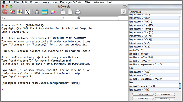
In Macintosh OS X the history items can be accessed and manipulated in an additional alternative fashion. The toolbar contains an icon that opens out a sidebar. This sidebar contains a list of the history items as shown in Figure 2-1.
At the foot of the sidebar are buttons that allow the loading or saving of history files. Any item can be pasted into the R console window by double clicking it.
You can still use the loadhistory(), savehistory(), and history() commands as described previously.
Editing History Files
The history files are saved on disk as plain text. This means that you can open them in any word processor and edit/manipulate them how you like. The history files saved by default have the .Rhistory extension. The files are stored in the default working directory unless you specified otherwise during the save operation. You can find out what the default directory is using the getwd() command described earlier.
When you save a history file and give it a name it becomes visible to the OS and to you in the file browser. The default history file has a name starting with a period and this makes it invisible in normal circumstances. The method you use to view these invisible files depends on the OS you are using.
In Macintosh you can check/alter the default history file by going to the Preferences menu. In Windows and Linux you must use a command like the following:
Sys.setenv('R_HISTFILE' = 'myhistory.Rhistory')You place the filename you require in quotes, remembering that the file will be saved in the default directory.
The history file does not grow infinitely; the number of entries is capped. You can set the limit from the preferences in Macintosh OS X, but in Windows or Linux you must use something along the following lines:
Sys.setenv('R_HISTSIZE' = 512)Unfortunately these commands only work while R is running and are “forgotten” when you quit. To make them permanent you need to get these commands to run automatically each time R is started. To do this search your home directory for a file called .Rprofile; it will be a hidden file. If this file does not exist, you can create one in a text editor and add the lines you require. These will be run when R opens.
You can check what the defaults for the history file and its size are by using the following commands, which work for all operating systems:
> Sys.getenv('R_HISTFILE')
          R_HISTFILE
"myhistory.Rhistory"
> Sys.getenv('R_HISTSIZE')
R_HISTSIZE
     "512"
If the default has not altered from the original, you will see a pair of quote marks. In practice there is little point altering the default history file. It is, however, useful to be able to save or load a set of commands as was described earlier (in the section “Saving and Recalling Lists of Commands”).
Saving Your Work in R
Once you begin working with R and creating named objects you will have a mixture of data items and results. You will want to save these to disk in order to work on them later or perhaps to share with others. You can use several methods to save your work. This section describes the most popular ones, including saving upon exit, saving to a disk, and saving to a text file.
Saving the Workspace on Exit
When you quit R, a message appears asking if you want to save the workspace image; it is a good habit to say yes. When you do, R saves all the objects currently in memory to the default workspace file (in your default working directory). The history items are also saved to their separate file.
This is a good way to keep all that you have been working on together so you can pick up where you left off. However, you can also save various objects to disk, either individually or in groups. This is especially useful if you are working on several projects and want to send data to a colleague or simply to keep items in separate places.
Saving Data Files to Disk
It is not really convenient to quit R every time you want to save your work to disk. Sometimes, if you are working on several items or projects at a time you may even want to save these separately. Fortunately, R provides a solution; you can save individual objects, or indeed all the objects, to disk at any time using the save() command.
Save Named Objects
The save() command operates like so:
save(list, file = 'filename')You need to specify a filename and it must be in quotes. The file will be saved to the current working directory by default. The list instruction can be in one of two forms: you can simply type the names of the objects you want to save separated with commas or you can link to a list of names created by some other means. Look at the examples that follow:
> save(bf, bf.lm, bf.beta, file = 'Desktop/butterfly.RData')
> save(list = ls(pattern = '^bf'), file = 'Desktop/butterfly.RData')
In the first case three objects were specified (bf, bf.lm, and bf.beta), and in the second example the ls() command was used to create a list of objects beginning with bf. In both cases, the output file was saved to the Desktop folder rather than the default.
Note that if you link to a list you must put the list instruction in the command explicitly, like so:
> mylist = c('bf', 'bf.beta', 'bf.lm')
> save(list = mylist, file = 'Desktop/butterfly.RData')
In this case the first command makes a simple list called mylist, which contains the names of the objects. The second command saves the objects to disk. Note also that the filename is completed by giving it an .RData extension; this is the preferred extension for saved data.
If you try to read an .RData file with a word processor, you will see a load of gibberish; data saved using the save() command is encoded. You are able to write files in a more generalized format using the write() command, as you see shortly.
Save Everything
If you want to save all the objects in memory, but there are a lot of them, it would be quite tedious to type all their names. R provides you with two alternative options:
save(list = ls(all=TRUE), file = 'filename')
save.image(file = 'filename')
In the first case everything is specified using the ls() command. The second example is a special command that allows you to save everything with a bit less typing. This is essentially what happens when you are asked to save the workspace when you quit R. If you do not specify a filename, the default is used; the filename defaults to “.RData”.
In both Windows and Macintosh OS X you can manipulate the workspace using the menu options. In Windows these are found under the File menu; in OS X they are in the Workspace menu.
Reading Data Files from Disk
When you save a file to disk, R saves the data in a binary format. This means that the file cannot be read by a regular word processor or text editor. You can read one of these binary files from within R using the load() command:
load(file = ‘filename.Rdata’)You need to put the filename in quotes (single or double, as long as the pair match) and remember to include the extension. The usual extension to use is .Rdata. If the file is not in your working directory the full path must be entered (all in the quotes). Alternatively, you can use the file.choose() instruction and select your file if you are using Windows or Macintosh operating systems.
load(file = file.choose())Once the file is read, any data objects that were saved in it are available and can be seen by using the ls() command.
It is also possible to load binary data items directly from your operating system by double-clicking the file you want. In Windows and Macintosh systems the .Rdata file extension should automatically become associated with R when you install the program. This is a useful way to open R because the only data that is loaded will be the data within the .Rdata file.
Creating data objects and transferring them to and from disk are really important activities. You will need to save data to disk in order to share with colleagues or simply to archive the data and keep your projects separate. In the following activity you get a chance to practice creating a simple data item, save it to disk, and reload it.
> ls()> savedata = c(9, 2, 4, 6, 5, 7, 9, 2, 1, 1, 7)> savedata
[1] 9 2 4 6 5 7 9 2 1 1 7> save(savedata, file = ‘savedata test.Rdata’)> rm(savedata)> load(file = ‘savedata test.Rdata’)> load(file = file.choose())> savedata
[1] 9 2 4 6 5 7 9 2 1 1 7Saving Data to Disk as Text Files
Saving your data in “R format” is extremely useful, especially if you are working on multiple projects; you are able to keep things separate. R maintains everything in memory though so if you have a very large amount of data, performance could suffer. In addition, there may well be times when you want to be able to save data items in a more universal format: for example, CSV or tab-delimited text. This can be useful to share data with colleagues who do not have R or to use for other purposes. For these reasons, it is available to save your data to disk as a text file instead of saving it to disk as a binary (R format) coded file.
Previously you met the read.table() and read.csv() commands (refer to the section “Reading Bigger Data Files”), which were used to transfer data into R. You can transfer data out of R using the write.table(), write.csv(), and cat() commands.
The command you use depends on what it is you want to save to disk. If you have a single vector of values you use write() or cat(); if you have a multiple column item containing several variables, you use write.table() or write.csv().
Writing Vector Objects to Disk
If you have a vector, you can use the write() command. The basic form of the command is the following:
write(x, file = "data", ncolumns = if(is.character(x)) 1 else 5, sep = " ")This looks a bit complicated because the ncolumns = part contains a conditional statement. This is because the if() statement creates a file with multiple columns according to the type of data. If the data are text, a single column is created. If the data are numeric, five columns are created (you can alter the number of columns). The items are separated by a space by default; you can change this by altering the sep = instruction. For example, the following code snippet contains a list of numbers. The write() command sees that these are numeric and creates five columns by default. The data are separated with commas.
> data7
 [1] 23.0 17.0 12.5 11.0 17.0 12.0 14.5  9.0 11.0  9.0 12.5 14.5 17.0  8.0 21.0
> write(data7, file = 'Desktop/data7.txt', sep = ',')
The resulting file looks like the following if viewed in a basic text editor:
23,17,12.5,11,17
12,14.5,9,11,9
12.5,14.5,17,8,21
If you want to create a single column you set the ncolumns = instruction to 1. If you want to create a single row you need to know how many items there are and set the number of columns to this value. You can do this automatically like so:
> write(data7, file = 'Desktop/data7.txt', sep = ',', ncolumns = length(data7))Here a command called length() was used, which determines how “long” the vector of data is. The resulting file looks like the following:
23,17,12.5,11,17,12,14.5,9,11,9,12.5,14.5,17,8,21A quicker way to achieve this result is to use the cat() command. Think of this as short for catalogue; just “print” the object and send it to a file.
> cat(data7, file = 'Desktop/data7.txt')In this instance the separator is left as a space (the default) and the data values are written as a simple row of numbers.
Writing Matrix and Data Frame Objects to Disk
If you have a matrix object or a data frame, you need to use the write.table() command. The basic command has various instructions that can be set as follows:
write.table(mydata, file = 'filename', row.names = TRUE, sep = ' ', col.names = TRUE)You replace the mydata part with the data item you want to write to disk. The filename needs to be in quotes and its location is relative to the current working directory. Each row of data is given an index number; most of the time you do not want to save this index to a file, so you need to alter the instruction to row.names = FALSE. If you want to make a file with columns separated by tabs, you put ‘ ’ in the sep = instruction. You can also specify the decimal point character using the dec = instruction.
If you want to make a CSV file, you could use the alternative write.csv() command. This is essentially the same but the default settings are slightly different:
write.csv(mydata, file = 'filename', row.names = TRUE, sep = ',', col.names = TRUE)The write.table() and write.csv() commands are most useful to save complex data items that contain multiple columns, such as you would expect to see in a spreadsheet. If you have a complex item like a matrix or a data frame object, this is the command you should use. List objects are also complex items, but they require special handling, as you see next.
Writing List Objects to Disk
Lists can be quite untidy and contain multiple items of varying sorts. Running an analytical command and storing the “result” generally creates a list, but you can also make a list as a way to tie together data items.
You can produce a text representation of the list using the dput() command and you can recall it using the dget() command. The two commands are simple:
dput(object, file = ““)
dget(file)
The following example shows a simple list. Here it is simply two numerical vectors but it could be a lot more complex:
> grass.l
$mow
[1] 12 15 17 11 15

$unmow
[1] 8 9 7 9

> dput(grass.l, file = 'Desktop/grass.txt')
The resulting file looks like this:
structure(list(mow = c(12L, 15L, 17L, 11L, 15L), unmow = c(8L,
9L, 7L, 9L)), .Names = c("mow", "unmow"))
This is not exactly what you would want in a spreadsheet, but it is the best you can do without pulling out the bits you want and re-arranging them. You can recall the list using dget(); in the following example a new object is created from the file using this command:
grass.list = dget(file = 'Desktop/grass.txt')The dput() command attempts to write an ASCII representation of your object to disk so that it can be recalled using the dget() command. The process does not always work smoothly. In general, data objects that are lists are recalled successfully but results of analyses are not. What generally happens is that the list object is reconstructed successfully, but certain attributes are lost. If your object is data this is not a problem, but if your result is a linear regression, for example, you may not be able to carry out some of the further commands that you may have wanted.
If you have complex results it is better to save them as .Rdata objects. If you want to use the text of a result you can easily copy it from the R console window and paste it into another program.
Converting List Objects to Data Frames
If you have a fairly simple list, perhaps containing several numerical samples, you can manipulate the list to produce a data frame and then save that to a text file.
Here is a simple list comprising of four numerical samples; you have met them all before:
> my.list
$mow
[1] 12 15 17 11 15

$unmow
[1] 8 9 7 9

$data3
 [1]  6  7  8  7  6  3  8  9 10  7  6  9

$data7
 [1] 23.0 17.0 12.5 11.0 17.0 12.0 14.5  9.0 11.0  9.0 12.5 14.5 17.0  8.0 21.0
Remember that you can check the structure of your object using the str() command like so:
> str(my.list)
List of 4
 $ mow  : int [1:5] 12 15 17 11 15
 $ unmow: int [1:4] 8 9 7 9
 $ data3: num [1:12] 6 7 8 7 6 3 8 9 10 7 ...
 $ data7: num [1:15] 23 17 12.5 11 17 12 14.5 9 11 9 ...
Because they are all numbers you could create a data frame that contained two columns, one for the actual numbers and one for the name of the sample each value relates to. To do this, you can use the stack() command like so:
> my.stack = stack(my.list)This creates a two-column data frame:
   values   ind
1      12   mow
2      15   mow
3      17   mow
4      11   mow
5      15   mow
6       8 unmow
7       9 unmow
8       7 unmow
9       9 unmow
10      6 data3
11      7 data3
12      8 data3
...
Not all of the data are shown here for brevity (try it out on your own and you will see the entire display). Notice that the column headings are values and ind. You can easily rename them to anything you like using the names() command:
> names(my.stack) = c('numbers', 'sample')Here the first column is changed to numbers and the second column is now called sample. You simply use the c() command to give the names you require.
To get back to the list from this new two-column data frame, you use the unstack() command like so:
> unstack(my.stack)
$data3
[1]  6  7  8  7  6  3  8  9 10  7  6  9

$data7
[1] 23.0 17.0 12.5 11.0 17.0 12.0 14.5 9.0 11.0 9.0 12.5 14.5 17.0 8.0 21.0

$mow
[1] 12 15 17 11 15

$unmow
[1] 8 9 7 9
This pulls the data apart back to its component samples, but you still need to create the list that “ties” the objects together. You do this like so:
> my.new.list = as.list(unstack(my.stack))In other words, you use the as.list() command to make the list from the unstacked data frame!
If you have several data vectors and want to create a list from them (rather than from a data frame like the preceding example), you use the as.list() command and give the object names that you want to include in the list:
> my.list = as.list(mow, unmow, data3, data7)However, this does not name the individual parts of the list (unlike the previous example where you had a data frame), so you need to add names afterwards like so:
> names(my.list) = c('mow', 'unmow', 'data3', 'data7')You can also use the list() command to do the same job, and in most ways they are identical.
Summary
- R can function as a simple calculator and the basic mathematical operators (for example, + - / *) can be used to perform math.
- You can store results of calculations for later use simply by typing a name to hold the result; the calculation then follows an = sign.
- You can create data objects from the keyboard, clipboard, or external data files using c(), scan(), and read.csv() commands.
- You can list objects that are ready for use using the ls() command and you can remove (delete) objects using the rm() command.
- There are different types of data, numerical and character. Data can exist in one of several forms; vectors are one-dimensional: matrixes and data frames are two-dimensional. List objects are loose collections of other objects.
- You can cycle through previous commands in the history using the up and down arrows. You can also save lists of commands to a file.
- You can write data from R to disk and save your work using the save() command. Other commands allow all items to be saved at once or for CSV files to be written.
Exercises
You can find answers to these exercises in Appendix A.
Buff tail: 10 1 37 5 12
Garden bee: 8 3 19 6 4
Red tail: 18 9 1 2 4
Honeybee: 12 13 16 9 10
Carder bee: 8 27 6 32 23What You Learned in This Chapter
| Topic | Key Points |
| Simple math: + - / * ^ log() cos() acos() abs() sqrt() pi() factorial() |
R can perform like a regular calculator and there are a range of mathematical operators and functions that can be used. Use help(Arithmetic) in R to get more information. |
| Assigning object names: Object.name = calculation Object.name <- calculation calculation -> Object.name |
Results of calculations can be stored as named objects. The = and <- symbols enable you to create an object from the result of the following calculation (in other words, you assign from right to left). The -> symbol enables you to assign the results of a calculation to a named object (that is, you assign from left to right). |
| Object names for example: data1 Data1 data.1 |
Objects are allowed names using all the letters a–z and uppercase A–Z as well as the numbers 0–9. A name must begin with a letter. The only punctuation mark allowed is a period. Names are case sensitive. |
| Making data: object.name = c(x, y, z) |
The c() command allows the concatenation of several items. It can be used to create data samples, for example. |
| Making data: object.name = scan() |
The scan() command allows data items to be entered from the keyboard, clipboard, or a simple text file. |
| Making data: object.name = read.table(file = ) |
The read.table() command allows a text file to be read from disk. The resulting object is a data frame with columns of equal length; short columns are padded out with NA.The read.csv() command is a special case of the command with defaults set for CSV files. |
| Listing objects: ls(pattern = regex)rm(item1, item2, …) |
The ls() command lists all the objects currently in memory. The rm() command removes objects (thereby deleting them). The list can use a regular expression and refine the result by listing only certain names. |
| Data type: numerical (numeric, integer)character (factor, character) |
Data can be in one of two major types, numerical for numbers or character for text. Number data can be integer or numeric. Text data can be classed as factor or character. The latter is a general type and items are shown enclosed in quotes. Factor data are text but not quoted. |
| Data form: vectordata framematrixlist |
Data can be in one of several forms. A one-dimensional structure is a vector. Data in 2D form can be a data frame or a matrix. In a matrix all the data of the same type. A data frame can contain mixtures of data (for example, numeric and factor). Missing values and “short” columns are padded with NA. A list object is a collection of other objects and can contain items of different lengths and types. |
| History commands: history()loadhistory()savehistory() |
Previously executed commands can be viewed using the up and down arrow keys. The entire history can be viewed using the history() command and files of commands can be loaded from or saved to disk. |
| Saving and loading data: save(x, y, z, …, file =)save.image(file =)write(x, file =)write.csv(data, file =)load(file =) |
When closing R all data can be saved to the default .RData file. The save() command can be used to save one or more objects to a file. The save.image() command can be used to save all objects to a file. The resulting files can be recalled using the load() command.A plain text representation of a data object can be saved to disk using the write() or write.csv() commands. |
| Finding data on disk: dir()getwd() setwd()file.choose() |
The dir() command allows the listing of files stored on disk. The working directory is where files are looked for and stored to by default. The location of the current working directory can be ascertained using getwd(). The working directory can be set to a new location using the setwd() command. Filenames must be specified explicitly but on Windows and Mac systems file.choose() can be used in place of a name, allowing a file to be selected by the user. |