
Chapter 9
KSC-net
Community Detection for Big Data Networks
Raghvendra Mall and Johan A.K. Suykens
Abstract
In this chapter, we demonstrate the applicability of the kernel spectral clustering (KSC) method for community detection in Big Data networks. We give a practical exposition of the KSC method [1] on large-scale synthetic and real-world networks with up to 106 nodes and 107 edges. The KSC method uses a primal–dual framework to construct a model on a smaller subset of the Big Data network. The original large-scale kernel matrix cannot fit in memory. So we select smaller subgraphs using a fast and unique representative subset (FURS) selection technique as proposed in Reference 2. These subsets are used for training and validation, respectively, to build the model and obtain the model parameters. It results in a powerful out-of-sample extensions property, which allows inferring of the community affiliation for unseen nodes. The KSC model requires a kernel function, which can have kernel parameters and what is needed to identify the number of clusters k in the network. A memory-efficient and computationally efficient model selection technique named balanced angular fitting (BAF) based on angular similarity in the eigenspace is proposed in Reference 1. Another parameter-free KSC model is proposed in Reference 3. In Reference 3, the model selection technique exploits the structure of projections in eigenspace to automatically identify the number of clusters and suggests that a normalized linear kernel is sufficient for networks with millions of nodes. This model selection technique uses the concept of entropy and balanced clusters for identifying the number of clusters k.
We then describe our software called KSC-net, which obtains the representative subset by FURS, builds the KSC model, performs one of the two (BAF and parameter-free) model selection techniques, and uses out-of-sample extensions for community affiliation for the Big Data network.
9.1 INTRODUCTION
In the modern era, with the proliferation of data and ease of its availability with the advancement of technology, the concept of Big Data has emerged. Big Data refers to a massive amount of information, which can be collected by means of cheap sensors and wide usage of the Internet. In this chapter, we focus on Big Data networks that are ubiquitous in current life. Their omnipresence is confirmed by the modern massive online social networks, communication networks, collaboration networks, financial networks, and so forth.
Figure 9.1 represents a synthetic network with 5000 nodes and a real-world YouTube network with over a million nodes. The networks are visualized using the Gephi software (https://gephi.org/).
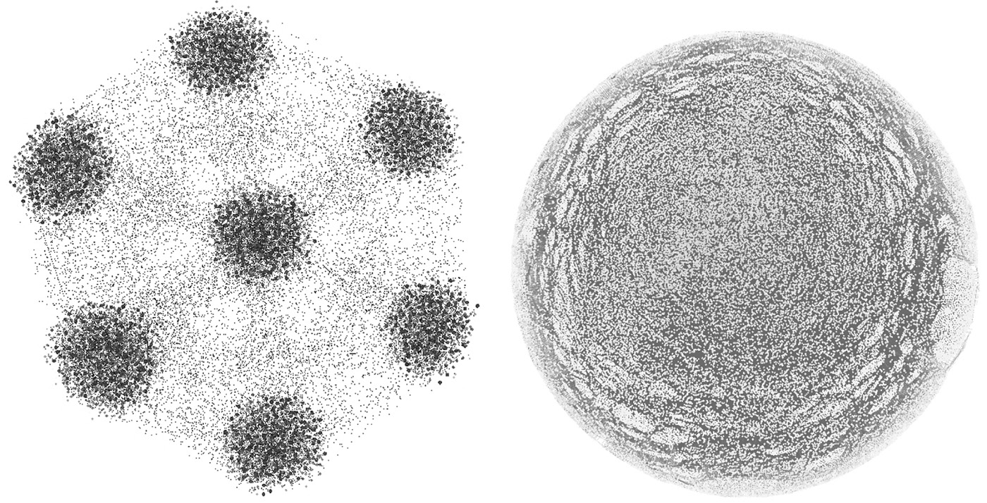
Real-world complex networks are represented as graphs G(V, E) where the vertices V represent the entities and the edges E represent the relationship between these entities. For example, in a scientific collaboration network, the entities are the researchers, and the presence or absence of an edge between two researchers depicts whether they have collaborated or not in the given network. Real-life networks exhibit community-like structure. This means nodes that are part of one community are densely connected to each other and sparsely connected to nodes belonging to other communities. This problem of community detection can also be framed as graph partitioning and graph clustering [4] and, of late, has received wide attention [5–16]. Among these techniques, one class of methods used for community detection is referred to as spectral clustering [13–16].
In spectral clustering, an eigen-decomposition of the graph Laplacian matrix (L) is performed. L is derived from the similarity or affinity matrix of the nodes in the network. Once the eigenvectors are obtained, the communities can be detected using the k-means clustering technique. The major disadvantage of the spectral clustering technique is that we need to create a large N × N kernel matrix for the entire network to perform unsupervised community detection. Here, N represents the number of nodes in the large-scale network. However, as the size of network increases, calculating and storing the N × N matrix becomes computationally infeasible.
A spectral clustering method based on weighted kernel principal component analysis (PCA) with a primal–dual framework is proposed in Reference 17. The formulation resulted in a model built on a representative subset of the data with a powerful out-of-sample extensions property. This representative subset captures the inherent cluster structure present in the data set. This property allows community affiliation for previously unseen data points in the data set. The kernel spectral clustering (KSC) method was extended for community detection on moderate-size graphs in Reference 11 and for large-scale graphs in Reference 1.
We use the fast and unique representative subset (FURS) selection technique introduced in Reference 2 for selection of the subgraphs on which we build our training and validation models (Figure 9.2). An important step in the KSC method is to estimate the model parameters, that is, kernel parameters, if any, and the number of communities k in the large-scale network. In the case of large-scale networks, the normalized linear kernel is an effective kernel as shown in Reference 18. Thus, we use the normalized linear kernel, which is parameter-less in our experiments. This saves us from tuning for an additional kernel parameter. In order to estimate the number of communities k, we exploit the eigen-projections in eigenspace to come up with a balanced angular fitting (BAF) criterion [1] and another self-tuned approach [3] where we use the concept of entropy and balance to automatically get k.
In this chapter, we give a practical exposition of the KSC method by first briefly explaining the steps involved and then showcasing its usage with the KSC-net software. We demonstrate the options available during the usage of KSC-net by means of two demos and explain the internal structure and functionality in terms of the KSC methodology.
9.2 KSC fOR Big Data NETWORKS
We first provide a brief description of the KSC methodology along with the FURS selection technique. We also explain the BAF and self-tuned model selection techniques. The notations used in this chapter are explained in Section 9.2.1.
9.2.1 Notations
- A graph is represented as G = (V, E) where V represents the set of nodes and E ⊆ V × V represents the set of edges in the network. The nodes represent the entities in the network, and the edges represent the relationship between them.
- The cardinality of the set V is given as N.
- The cardinality of the set E is given as Etotal.
- The adjacency matrix A is an N × N sparse matrix.
- The affinity/kernel matrix of nodes is given by Ω, and the affinity matrix of projections is depicted by S.
- For unweighted graphs, Aij = 1 if (vi, vj) ∈ E, else Aij = 0.
- The subgraph generated by the subset of nodes B is represented as G(B). Mathematically, G(B) = (B, Q) where B ⊂ V and Q = (S × S) ∩ E represents the set of edges in the subgraph.
- The degree distribution function is given by f(V). For the graph G, it can written as f(V), while for the subgraph B, it can be presented as f(B). Each vertex vi ∈ V has a degree represented as f(vi).
- The degree matrix is represented as D. It is a diagonal matrix with diagonal entries .
- The adjacency list corresponding to each vertex vi ∈ V is given by xi = A(:,i).
- The set of neighboring nodes of a given node vi is represented by Nbr(vi).
- The median degree of the graph is represented as M.
The KSC methodology comprises three major steps:
- Building a model on the training data
- Identifying the model parameters using the validation data
- The out-of-sample extension to determine community affiliation for the unseen test set of nodes
9.2.2 FURS Selection
Nodes that have higher-degree centrality or more connections represent the presence of more influence and have the tendency to be located in the center of the network. The goal of the FURS selection technique is to select several such nodes of high-degree centrality from different dense regions in the graph to capture the inherent community structure present in the network. However, this problem of selection of such a subset (B) takes nondeterministic polynomial time (NP-hard) and is formulated as
(9.1)
where D(vj) represents the degree centrality of the node vj, s is the size of the subset, ci represents the ith community, and k represents the number of communities in the network that cannot be determined explicitly beforehand.
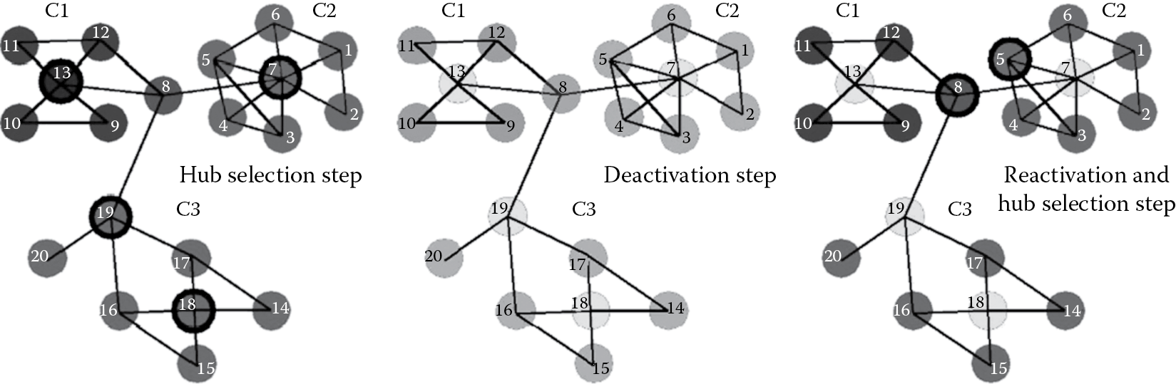
The FURS selection technique is a greedy solution to the aforementioned problem. It is formulated as an optimization problem where we maximize the sum of the degree centrality of the nodes in the selected subset B, such that neighbors of the selected node are deactivated or cannot be selected in that iteration. By deactivating its neighborhood, we move from one dense region in the graph to another, thereby approximately covering all the communities in the network. If all the nodes are deactivated in one iteration and we have not yet reached the required subset size s, then these deactivated nodes are reactivated, and the procedure is repeated till we reach the required size s. The optimization problem is formulated in Equation 9.2:
(9.2)
where st is the size of the set of nodes selected by FURS during iteration t.
Several approaches have been proposed for sampling a graph, including References 2, 19 through 21. The FURS selection approach was proposed in Reference 2 and used in Reference 1. A comprehensive comparison of various sampling techniques has been explained in detail in Reference 2. We use the FURS selection technique in KSC-net software for training and validation set selection.
9.2.3 KSC Framework
For large-scale networks, the training data comprise the adjacency list of all the nodes vi, i = 1,…,Ntr. Let the training set of nodes be represented by Vtr and the training set cardinality be Ntr. The validation and test sets of nodes are represented by Vvalid and Vtest, respectively. The cardinalities of these sets are Nvalid and Ntest, respectively. These sets of adjacency lists can efficiently be stored in the memory as real-world networks are highly sparse and there are limited connections for each node vi ∈ Vtr. The maximum length of the adjacency list can be equal to N. This is the case when a node is connected to all the other nodes in a network.
9.2.3.1 Training Model
For Vtr training nodes selected by the FURS selection technique, , such that . Here, xi represents the adjacency list of the ith training node. Given and a user-defined maxk (maximum number of clusters in the network), the primal formulation of the weighted kernel PCA [17] is given by
(9.3)
where are the projections onto the eigenspace; l = 1;…; maxk − 1 indicates the number of score variables required to encode the maxk communities; is the inverse of the degree matrix associated to the kernel matrix Ω; Φ is the Ntr × dh feature matrix; and and are the regularization constants. We note that Ntr ≪ N, that is, the number of nodes in the training set is much less than the total number of nodes in the large-scale network. The kernel matrix Ω is obtained by calculating the similarity between the adjacency list of each pair of nodes in the training set. Each element of Ω, denoted as Ωij = K(xi, xj) = ϕ(xi)⊺ϕ(xj), is obtained by calculating the cosine similarity between the adjacency lists xi and xj. Thus, can be calculated efficiently using notions of set unions and intersections. This corresponds to using a normalized linear kernel function [22]. The clustering model is then represented by
(9.4)
where is the mapping to a high-dimensional feature space of dimension dh; bl are the bias terms; and l = 1;…;maxk − 1. However, for large-scale networks, we can utilize the explicit expression of the underlying feature map and dh = N. Since the KSC formulation is valid for any positive definite kernel, we use a normalized linear kernel function to avoid any kernel parameter. The projections represent the latent variables of a set of maxk − 1 binary cluster indicators given by , which can be combined with the final groups using an encoding/decoding scheme. The dual problem corresponding to this primal formulation is
(9.5)
where . The α(l) are the dual variables, and the kernel function plays the role of similarity function.
9.2.3.2 Model Selection
KSC-net provides the user with the option to select one of the two model selection techniques, that is, the BAF criterion [1] or the self-tuned procedure [3].
Algorithm 1: BAF Model Selection Criterion
Data: Given codebook C , maxk, and .
Result: Maximum BAF value and optimal k.
1 foreach k ∈ (2, maxk] do
2 Calculate the cluster memberships of training nodes using codebook C .
3 Get the clustering Δ = {C1,…,Ck} and calculate cluster mean ui for each Ci.
4 For each validation node validi, obtain , where .
5 Maintain dictionary .
6 Obtain clustering for the validation nodes.
7 Define BAF as .
8 end
9 Save the maximum BAF value along with the corresponding k.
9.2.3.3 Out-of-Sample Extension
Ideally, when the communities are nonoverlapping, we will obtain k well-separated communities, and the normalized Laplacian has k piecewise constant eigenvectors. This is because the multiplicity of the largest eigenvalue, that is, 1, is k as depicted in Reference 23. In the case of KSC due to the centering matrix MD, the eigenvectors have zero mean, and the optimal threshold for binarizing the eigenvectors is self-determined (equal to 0). So we need k − 1 eigenvectors. However, in real-world networks, the communities exhibit overlap and do not have piecewise constant eigenvectors.
Algorithm 2: Algorithm to Automatically Identify k Communities
Data: .
Result: The number of clusters k in the given large-scale network.
1 Construct S using the projection vectors and their CosDist().
2 Set td = [0.1, 0.2, …, 1].
3 foreach t ∈ td do
4 Save S in a temporary variable R, that is, R : = S and SizeCt = [].
5 while S is not an empty matrix do
6 Find with maximum number of nodes whose cosine distance is < t.
7 Determine the number of these nodes and append it to SizeCt.
8 Remove rows and columns corresponding to the indices of these nodes.
9 end
10 Calculate the entropy and expected balance from SizeCt as in Reference 3.
11 Calculate the F-measure F(t) using entropy and balance.
12 end
13 Obtain the threshold corresponding to which F-measure is maximum as maxt.
14 Estimate k as the number of terms in the vector SizeCmaxt.
The decoding scheme consists of comparing the cluster indicators obtained in the validation/test stage with the codebook C and selecting the nearest codebook based on Hamming distance. This scheme corresponds to the error correcting output codes (ECOC) decoding procedure [24] and is used in out-of-sample extensions as well.
The out-of-sample extension is based on the score variables that correspond to the projections of the mapped out-of-sample nodes onto the eigenvectors found in the training stage. The cluster indicators can be obtained by binarizing the score variables for the out-of-sample nodes as
(9.6)
where l = 1;…; k − 1; Ωtest is the Ntest × Ntr kernel matrix evaluated using the test nodes with entries Ωr,i = K(xr, xi); r = 1;…; Ntest; and i = 1;…; Ntr. This natural extension to out-of-sample nodes is the main advantage of KSC. In this way, the clustering model can be trained, validated, and tested in an unsupervised learning procedure. For the test set, we use the entire network. If the network cannot fit in memory, we divide it into blocks to calculate the cluster memberships for each test block in parallel.
9.2.4 Practical Issues
In this chapter, all the graphs are undirected and unweighted unless otherwise specified. We conducted all our experiments on a machine with a 12 GB RAM, 2.4 GHz Intel Xeon processor. The maximum cardinality allowed for the training (Ntr) and the validation set (Nvalid) is 5000 nodes. This is because the maximum-size kernel matrix that we can store in the memory of our PC is 5000 × 5000. We use the entire network as test set Vtest. We perform the community affiliation for unseen nodes in an iterative fashion by dividing Vtest into blocks of 5000 nodes. This is because the maximum-size Ωtest that we can store in the memory of our PC is 5000 × 5000. However, this operation can easily be extended to a distributed environment and performed in parallel.
9.3 KSC-net SOFTWARE
The KSC-net software is available for Windows and Linux platforms at ftp://ftp.esat.kuleuven.be/SISTA/rmall/KSCnet_Windows.tar.gz and ftp://ftp.esat.kuleuven.be/SISTA/rmall/KSCnet_Linux.tar.gz, respectively. In our demos, we use a benchmark synthetic network obtained from Reference 9 and an anonymous network available freely from the Stanford SNAP library, http://snap.stanford.edu/data/index.html.
9.3.1 KSC Demo on Synthetic Network
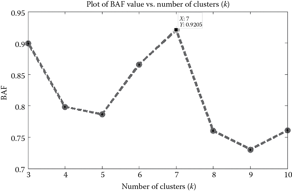
We first provide a demo script to showcase the KSC methodology on a synthetic network that has 5000 nodes and 124,756 edges. The network comprises communities that are known beforehand and act as ground truth. We provide the demo script below. Figure 9.3 is also obtained as an output of the demo script to show the effectiveness of the BAF model selection criterion. From Figure 9.3, we can observe that the maximum BAF value is 0.9205, and it occurs corresponding to k = 7, which is equal to the actual number of communities in the network. The adjusted Rand index (ARI) [25] value is 0.999, which means that the community membership provided by the KSC methodology is as good as the original ground truth.
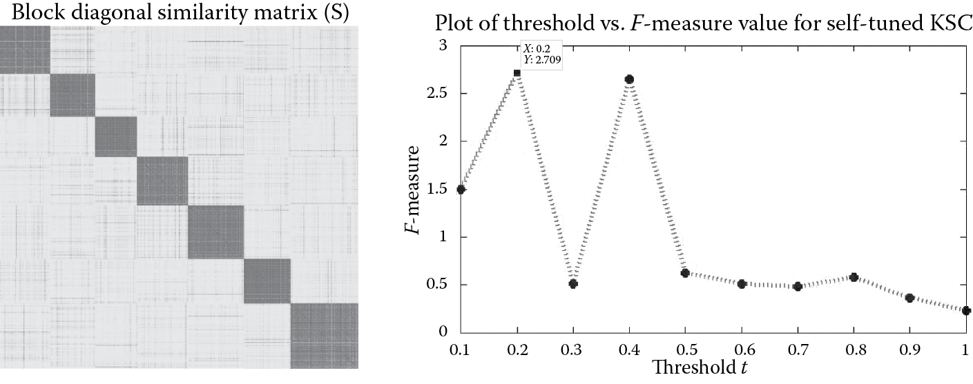
If we put mod_sel = 'Self' in the demo script of Algorithm 3, then we perform the self-tuned model selection. It uses the concept of entropy and balance clusters to identify the optimal number of clusters k in the network. Figure 9.4 showcases the block diagonal affinity matrix S generated from the eigen-projections of the validation set using the self-tuned model selection procedure. From Figure 9.4, we can observe that there are seven blocks in the affinity matrix S. In order to calculate the number of these blocks, the self-tuned procedure uses the concept of entropy and balance together as an F-measure. Figure 9.4 shows that the F-measure is maximum for threshold t = 0.2, for which it takes the value 2.709. The number of clusters k identified corresponding to this threshold value is 7, which is equivalent to the number of ground truth communities.
Algorithm 3: Demo Script for Synthetic Network Using BAF Criterion
Data:
netname = 'network';//Name of the file and extension should be '.txt'
baseinfo = 1; //Ground truth exists
cominfo = 'community'; //Name of ground truth file and extension should be '.txt'
weighted = 0; //Whether a network is weighted or unweighted
frac_network = 15; //Percentage of network to be used as training and //validation set
maxk = 10; //maxk is maximum value of k to be used in eigen-decomposition, use //maxk = 10 for k < = 10 else use maxk = 100
mod_sel = 'BAF'; //Method for model selection (options are 'BAF' or 'Self')
output = KSCnet(netname,baseinfo,cominfo,weighted,frac_network,maxk,mod_sel);
Result
output = 1; //When community detection operation completes
netname_numclu_mod_sel.csv; //Number of clusters detected
netname_outputlabel.csv; //Cluster labels assigned to the nodes
netname_ARI.csv; //Valid only when ground truth is known, provides information //about ARI and number of communities covered
9.3.2 KSC Subfunctions
We briefly describe some of the subfunctions that are called within the KSCnet() function. First, the large-scale network is provided as an edge list with or without the ground truth information; we convert the edge list into a sparse adjacency matrix A. The frac network provides information about what percentage of the total number of nodes in the network is to be used as a training and validation set. We put a condition to check that the Ntr or Nvalid cannot exceed a maximum value of 5000. We then use the “system” command to run the FURS selection technique as it is implemented in the scripting language Python. The Python prerequisites are provided in the “ReadMe.txt.” Figure 9.5 demonstrates the output obtained when the FURS selection technique is used for selecting the training and validation set.
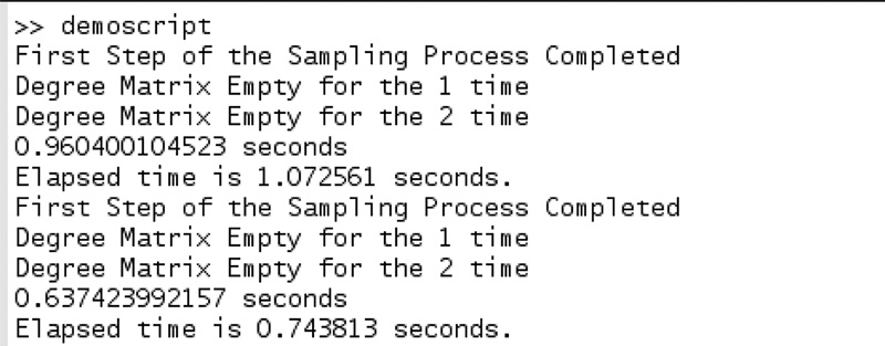
From Figure 9.5, we can observe that the statement “First Step of the Sampling Process Completed” appears twice (once for training and once for validation).
- KSCmod. The KSCmod function takes as input a Boolean state variable to determine whether it is the training or test phase. If it is 0, then we provide as input the training and validation set; otherwise, the input is the training and test sets. It also takes as input maxk and the eigenvalue decomposition algorithm (options are “eig” or “eigs”). It calculates the kernel matrix using a Python code and then solves the eigen-decomposition problem to obtain the model. Output is the model along with its parameters, training/validation/test set eigen-projections, and codebook C . For the validation set, we also obtain the community affiliation corresponding to maxk, but for the test set, we obtain cluster membership corresponding to optimal k.
- KSCcodebook. KSCcodebook takes as input the eigen-projections and eigenvectors. It takes the sign of these eigen-projections, calculates the top k most frequent code words, and outputs them as a codebook. It also estimates the cluster memberships for the training nodes using the KSCmembership function.
- KSCmembership. KSCmembership takes as input the eigen-projections of the train/validation/test set and codebook. It takes a sign of these eigen-projections and calculates the Hamming distance between the codebook and the sign (ei). It assigns the corresponding node to that cluster with which it has minimum Hamming distance.
In the case of the BAF model selection criterion, we utilize the KSCcodebook and KSCmembership functionality to estimate the optimal number of communities k in the large-scale network. However, the “Self” model selection technique works independent of these functions and uses the concept of entropy and balance to calculate the number of block diagonals in the affinity matrix S generated by the validation set eigen-projections after reordering by means of the ground truth information. Figure 9.6 represents a snippet that we obtain when trying to identify the optimal number of communities k in the large-scale network.
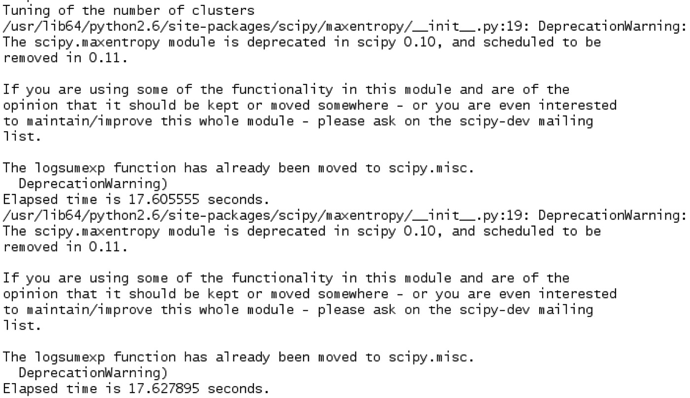
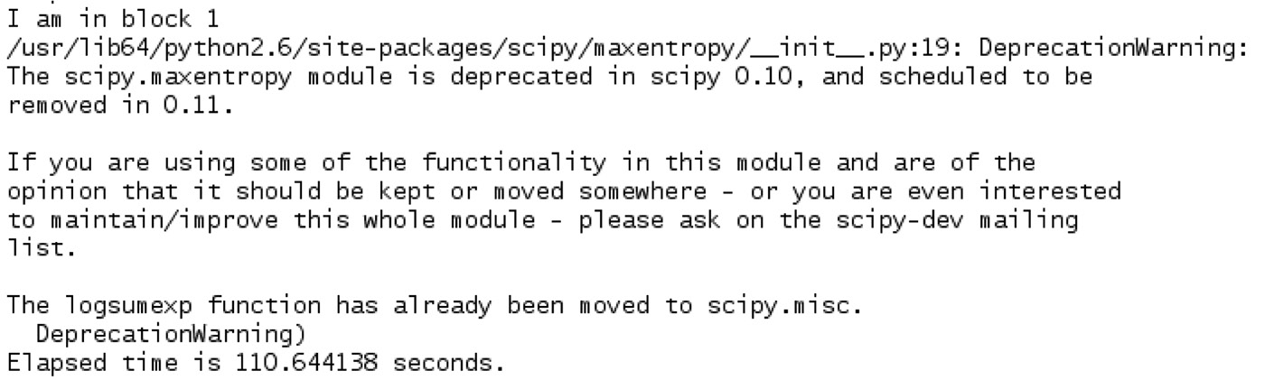
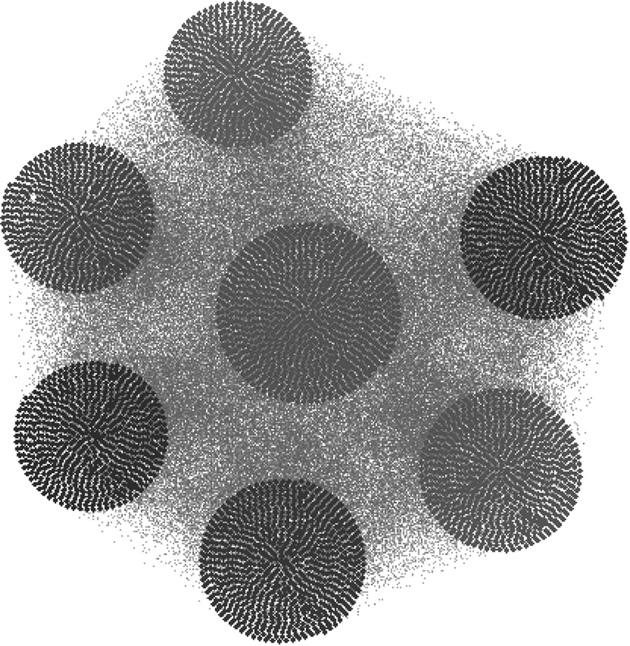
In Figure 9.6, we observe a “DeprecationWarning,” which we ignore as it is related to some functionality in the “scipy” library, which we are not using. We also observe that we obtained “Elapsed time…” at two places. Once, it occurs after building the training model, and the second time, it appears after we have performed the model selection using the validation set. Figure 9.7 represents the time required to obtain the test set community affiliation. Since there are only 5000 nodes in the entire network and we divide the test set into blocks of 5000 nodes due to memory constraints, we observe “I am in block 1” in Figure 9.7. Figure 9.8 showcases the community-based structure for the synthetic network. We get the same result in either case when we use the BAF selection criterion or the “Self” selection technique.
9.3.3 KSC Demo on Real-Life Network
We provide a demo script to showcase the KSC methodology on a real-life large-scale YouTube network that has 1,134,890 nodes with 2,987,624 edges. The network is highly sparse. It is a social network where users form friendship with each other and can create groups that other users can join. We provide the demo script below.
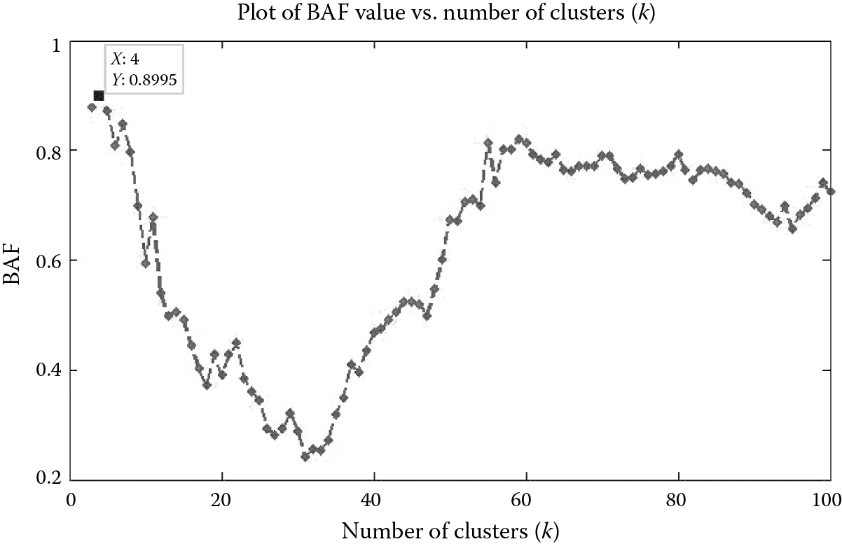
Figure 9.9 shows the effectiveness of the BAF model selection criterion on the YouTube social network. From Figure 9.9, we observe that there are multiple local peaks on the BAF-versus-k curve. However, we select the peak corresponding to which the BAF value is maximum. This occurs at k = 4 for the BAF value of 0.8995. Since we provide the cluster memberships for the entire network to the end user, the end user can use various internal quality criteria to estimate the quality of the resulting communities.
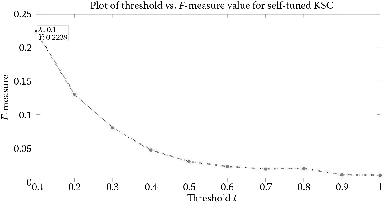
If we put mod_sel = 'Self' in the demo script of Algorithm 4, then we would be using the parameter-free model selection technique. Since the ground truth communities are not known beforehand, we try to estimate the block diagonal structure using the greedy selection technique mentioned in Algorithm 2 to determine the SizeCt vector. Figure 9.10 shows that the F-measure is maximum for t = 0.1, for which it takes the value 0.224. The number of communities k identified corresponding to this threshold value is 36 (Figure 9.11).
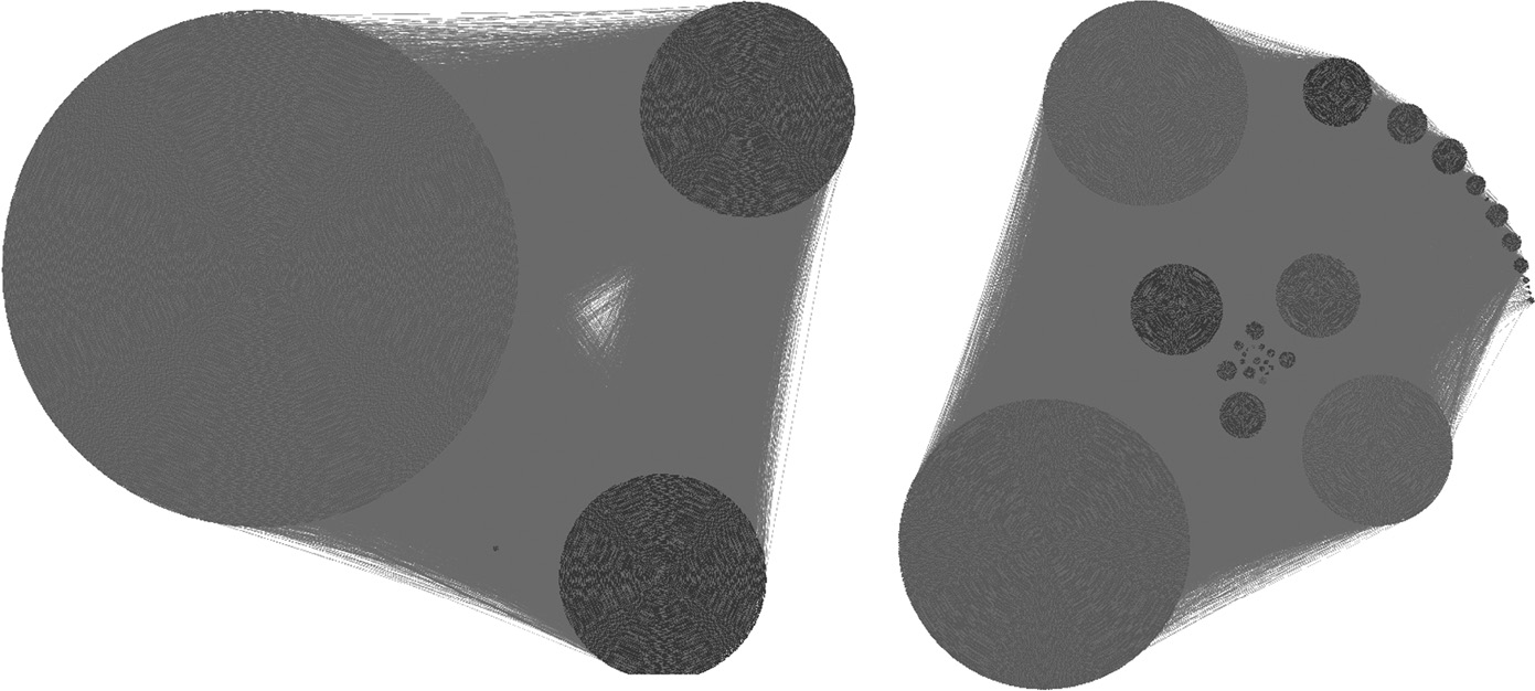
Community structure detected for the YouTube network by “BAF” and “Self” model selection techniques respectively visualized using the software provided in Reference 26. (From Lancichinetti, A. et al., Plos One, 6(e18961), 2011.)
Algorithm 4: Demo Script for YouTube Network Using BAF Criterion
Data:
netname = 'youtube_mod'; //Name of the file and extension should be '.txt'
baseinfo = 0; //Ground truth does not exists
cominfo = []; //No ground truth file so empty set as input
weighted = 0; //Whether a network is weighted or unweighted
frac_network = 10; //Percentage of network to be used as training and //validation set
maxk = 100; //maxk is maximum value of k to be used in eigen-decomposition, //use maxk = 10 for k < = 10 else use maxk = 100
mod_sel = 'BAF'; //Method for model selection (options are 'BAF' or 'Self')
output = KSCnet(netname,baseinfo,cominfo,weighted,frac_network,maxk,mod_sel);
Result:
output = 1; //When community detection operation completes
netname_numclu_mod_sel.csv; //Number of clusters detected
netname_outputlabel.csv; //Cluster labels assigned to the nodes
9.4 CONCLUSION
In this chapter, we gave a practical exposition of a methodology to perform community detection for Big Data networks. The technique was built on the concept of spectral clustering and referred to as KSC. The core concept was to build a model on a small representative subgraph that captured the inherent community structure of the large-scale network. The subgraph was obtained by the FURS [2] selection technique. Then, the KSC model was built on this subgraph. The model parameters were obtained by one of the two techniques: (1) BAF criterion or (2) self-tuned technique. The KSC model has a powerful out-of-sample extensions property. This property was used for community affiliation of previously unseen nodes in the Big Data network. We also explained and demonstrated the usage of the KSC-net software, which uses the KSC methodology as the underlying core concept.
Acknowledgments
EU: The research leading to these results has received funding from the European Research Council under the European Union’s Seventh Framework Programme (FP7/2007-2013)/ERC AdG A-DATADRIVE-B (290923). This chapter reflects only the authors’ views; the Union is not liable for any use that may be made of the contained information. Research Council KUL: GOA/10/09 MaNet, CoE PFV/10/002 (OPTEC), BIL12/11T; PhD/postdoc grants. Flemish government—FWO: projects G.0377.12 (structured systems), G.088114N (tensor-based data similarity); PhD/postdoc grants. IWT: project SBO POM (100031); PhD/postdoc grants. iMinds Medical Information Technologies: SBO 2014. Belgian Federal Science Policy Office: IUAP P7/19 (DYSCO, dynamical systems, control and optimization, 2012–2017).
References
1. R. Mall, R. Langone and J.A.K. Suykens; Kernel spectral clustering for Big Data networks. Entropy (Special Issue: Big Data), 15(5):1567–1586, 2013.
2. R. Mall, R. Langone and J.A.K. Suykens; FURS: Fast and Unique Representative Subset selection retaining large scale community structure. Social Network Analysis and Mining, 3(4):1–21, 2013.
3. R. Mall, R. Langone and J.A.K. Suykens; Self-tuned kernel spectral clustering for large scale networks. In Proceedings of the IEEE International Conference on Big Data (IEEE BigData 2013). Santa Clara, CA, October 6–9, 2013.
4. S. Schaeffer; Algorithms for nonuniform networks. PhD thesis. Espoo, Finland: Helsinki University of Technology, 2006.
5. L. Danaon, A. Diáz-Guilera, J. Duch and A. Arenas; Comparing community structure identification. Journal of Statistical Mechanics: Theory and Experiment, 9:P09008, 2005.
6. S. Fortunato; Community detection in graphs. Physics Reports, 486:75–174, 2009.
7. A. Clauset, M. Newman and C. Moore; Finding community structure in very large scale networks. Physical Review E, 70:066111, 2004.
8. M. Girvan and M. Newman; Community structure in social and biological networks. Proceedings of the National Academy of Sciences of the United States of America, 99(12):7821–7826, 2002.
9. A. Lancichinetti and S. Fortunato; Community detection algorithms: A comparative analysis. Physical Review E, 80:056117, 2009.
10. M. Rosvall and C. Bergstrom; Maps of random walks on complex networks reveal community structure. Proceedings of the National Academy of Sciences of the United States of America, 105:1118–1123, 2008.
11. R. Langone, C. Alzate and J.A.K. Suykens; Kernel spectral clustering for community detection in complex networks. In IEEE WCCI/IJCNN, pp. 2596–2603, 2002.
12. V. Blondel, J. Guillaume, R. Lambiotte and L. Lefebvre; Fast unfolding of communities in large networks. Journal of Statistical Mechanics: Theory and Experiment, 10:P10008, 2008.
13. A.Y. Ng, M.I. Jordan and Y. Weiss; On spectral clustering: Analysis and an algorithm. In Proceedings of the Advances in Neural Information Processing Systems, Dietterich, T.G., Becker, S., Ghahramani, Z., editors. Cambridge, MA: MIT Press, pp. 849–856, 2002.
14. U. von Luxburg; A tutorial on spectral clustering. Statistics and Computing, 17:395–416, 2007.
15. L. Zelnik-Manor and P. Perona; Self-tuning spectral clustering. In Advances in Neural Information Processing Systems, Saul, L.K., Weiss, Y., Bottou, L., editors. Cambridge, MA: MIT Press, pp. 1601–1608, 2005.
16. J. Shi and J. Malik; Normalized cuts and image segmentation. IEEE Transactions on Pattern Analysis and Intelligence, 22(8):888–905, 2000.
17. C. Alzate and J.A.K. Suykens; Multiway spectral clustering with out-of-sample extensions through weighted kernel PCA. IEEE Transactions on Pattern Analysis and Machine Intelligence, 32(2):335–347, 2010.
18. L. Muflikhah; Document clustering using concept space and concept similarity measurement. In ICCTD, pp. 58–62, 2009.
19. A. Maiya and T. Berger-Wolf; Sampling community structure. In WWW, pp. 701–710, 2010.
20. U. Kang and C. Faloutsos; Beyond ‘caveman communities’: Hubs and spokes for graph compression and mining. In Proceedings of ICDM, pp. 300–309, 2011.
21. N. Metropolis, A. Rosenbluth, M. Rosenbluth, A. Teller and E. Teller; Equation of state calculations by fast computing machines. Journal of Chemical Physics, 21(6):1087–1092, 1953.
22. J.A.K. Suykens, T. Van Gestel, J. De Brabanter, B. De Moor and J. Vandewalle; Least Squares Support Vector Machines. Singapore: World Scientific, 2002.
23. F.R.K. Chung; Spectral Graph Theory. Providence, RI: American Mathematical Society, 1997.
24. J. Baylis; Error Correcting Codes: A Mathematical Introduction. Boca Raton, FL: CRC Press, 1988.
25. R. Rabbany, M. Takaffoli, J. Fagnan, O.R. Zaiane and R.J.G.B. Campello; Relative validity criteria for community mining algorithms. In International Conference on Advances in Social Networks Analysis and Mining (ASONAM), pp. 258–265, 2012.
26. A. Lancichinetti, F. Radicchi, J.J. Ramasco and S. Fortunato; Finding statistically significant communities in networks. PLoS One, 6:e18961, 2011.