
Chapter 14
Managing Big Trajectory Data
Online Processing of Positional Streams
Kostas Patroumpas and Timos Sellis
Abstract
As smartphones and GPS-enabled devices proliferate, location-based services become all the more important in social networking, mobile applications, advertising, traffic monitoring, and many other domains. Managing the locations and trajectories of numerous people, vehicles, vessels, commodities, and so forth must be efficient and robust, since this information must be processed online and should provide answers to users’ requests in real time. In this geostreaming context, such long-running continuous queries must be repeatedly evaluated against the most recent positions relayed by moving objects, for instance, reporting which people are now moving in a specific area or finding friends closest to the current location of a mobile user. In essence, modern processing engines must cope with huge amounts of streaming, transient, uncertain, and heterogeneous spatiotemporal data, which can be characterized as big trajectory data. In this chapter, we examine Big Data processing techniques over frequently updated locations and trajectories of moving objects. Rapidly evolving trajectory data pose several research challenges with regard to their acquisition, storage, indexing, analysis, discovery, and interpretation in order to be really useful for intelligent, cost-effective decision making. Indeed, the Big Data issues regarding volume, velocity, variety, and veracity also arise in this case. Thus, we foster a close synergy between the established stream processing paradigm and spatiotemporal properties inherent in motion features. Taking advantage of the spatial locality and temporal timeliness that characterize each trajectory, we present methods and heuristics from our recent research results that address such problems. We highlight certain aspects of big trajectory data management through several case studies. Regarding volume, we suggest single-pass algorithms that can summarize each object’s course into succinct, reliable representations. To cope with velocity, an amnesic trajectory approximation structure may offer fast, multiresolution synopses by dropping details from obsolete segments. Detection of objects that travel together can lead to trajectory multiplexing, hence reducing the variety inherent in raw positional data. As for veracity, we discuss a probabilistic method for continuous range monitoring against user locations with varying degrees of uncertainty, due to privacy concerns in geosocial networking. Last, but not least, as we are heading toward a next-generation framework in trajectory data management, we point out interesting open issues that may provide rich opportunities for innovative research and applications.
14.1 Introduction
Nowadays, hundreds of millions of GPS-enabled devices are in use globally. The amount of information exchanged on a daily basis is in the order of terabytes for several social networks (like Facebook or Twitter) or financial platforms (e.g., New York Stock Exchange). Billions of radio-frequency identification (RFID) tags are generated per day, and millions of sensors collect measurements in diverse application domains, ranging from meteorology and biodiversity to energy consumption, battlefield monitoring, and many more. These staggering figures are expected to double every 2 years over the next decade, as the number of Internet users, smartphone holders, online customers, and networked sensors is growing at a very fast rate. Quite often, this information also includes a spatial aspect, either explicitly in the form of coordinates (from GPS, RFID, or global system for mobile communications [GSM]) or implicitly (via geo-tagged photos or addresses). As smartphones and GPS-enabled devices proliferate and related platforms penetrate into the market, managing the bulk of rapidly accumulating traces of objects’ movement becomes all the more crucial in modern, high-availability applications. Such location-based services (LBSs) are capable of identifying the geographical location of a mobile device and then providing services based on that location. Platforms for traffic surveillance and fleet management, mobile applications in tourism or advertising, notification systems for natural resources and hazards, tracing services for stolen objects or elder people, and so forth must cope with huge amounts of such flowing, uncertain, and heterogeneous spatiotemporal data.
These data sets can certainly be characterized as Big Data [1], not only because of their increasingly large volumes but also due to their volatility and complexity, which make their processing and analysis quite difficult, if not impossible, through traditional data management tools and applications. Obviously, it is too hard for a centralized server to sustain massive amounts of positional updates from a multitude of people, vehicles, vessels, containers, and so forth, which may also affect network traffic and load balancing. The main challenge is how such fluctuating, transient, and possibly unbounded positional data streams can be processed in online fashion. In such a geostreaming context, it is important to provide incremental answers to continuous queries (CQs), that is, to various and numerous user requests that remain active for long and require their results to be refreshed upon changes in the incoming data [2]. There are several types of location-aware CQs [3,4] that examine spatial relationships against the current locations of numerous moving objects. For instance, a continuous range search must report which objects are now moving in a specific area of interest (e.g., vehicles in the city center). A mobile user who wishes to find k of his/her friends that are closest to his/her current location is an example of a continuous k-nearest neighbor (k-NN) search. As the monitored objects are moving and their relative positions are changing, new results must be emitted, thus cancelling or modifying previous ones (e.g., 5 min after the previous answer to this k-NN CQ, the situation has changed, and another friend is now closer to him/her).
In the course of time, many locations per object are being accumulated and can actually be used to keep track of its trace. Of course, it is not realistic to maintain a continuous trace of each object, since practically, point samples can only be collected from the respective data source at distinct time instants (e.g., every few seconds, a car sends its location measured by a GPS device). Still, these traces can be a treasure trove for innovative data analysis and intelligent decision making. In fact, data exploration and trend discovery against such collections of evolving trajectories are also crucial, beyond their effective storage or the necessity for timely response to user requests. From detection of flocks [5] or convoys [6] in fleet management to clustering [7] for wildlife protection, similarity joins [8] in vehicle traces for carpooling services, or even identification of frequently followed routes [9,10] for effective traffic control, the prospects are enormous.
The core challenges regarding Big Data [11] are usually described through the well-known three Vs, namely, volume, velocity, and variety, although in Reference 12, it was proposed to include a fourth one for veracity. In the particular case of big trajectory data collected from moving objects, these challenges may be further specified as follows:
- Volume. If numerous vehicles, parcels, smartphones, animals, and so forth are monitored and their locations get relayed very frequently, then large amounts of positional data are being captured. Hence, the processing mechanism must be scalable, as the sheer volume of positional data may be overwhelming and could exceed several terabytes per day. Further, processing every single position incurs some overhead but does not necessarily convey significant movement changes (e.g., if a vessel moves along a straight line for some time), so opportunities exist for data compression because of similar redundancies in the input.
- Velocity. As data are generated continuously at various rates and are inherently streaming in a time-varying fashion, they must be handled and processed in real time. However, typical spatiotemporal queries like range, k-NN, and so forth are costly, and their results should not be computed from scratch upon admission of fresh input. Ideally, evaluation of the current batch of positional data must be completed before the next one arrives, in order to provide timely results and also keep in pace with the incoming streaming locations.
- Variety. Data can actually come from multiple, possibly heterogeneous sources and may be represented in various types or formats, either structured (e.g., as relational tuples, sensor readings) or unstructured (logs, text messages, etc.). Location could have differing semantics, for example, positions may come from both GPS devices and GSM cells; hence, accuracy may vary widely, up to hundreds of meters. Besides, these dynamic positional data might also require interaction with static data sets, for example, for matching vehicle locations against the underlying road network. Handling the intricacies of such data, eliminating noise and errors (e.g., positional outliers), and interpreting latent motion patterns are nontrivial tasks and may be subject to assumptions at multiple stages of the analysis.
- Veracity. Due to privacy concerns, hiding a user location and not just his/her identity is important. Hence, positional data may be purposely noisy, obfuscated, or erroneous in order to avoid malicious or inappropriate use (e.g., prevent locating of people or linking them to certain groups in terms of social, cultural, or market habits). But handling such uncertain, incomplete information adds too much complexity to processing; hence, results cannot be accurate and are usually associated with a probabilistic confidence margin.
To address such challenging research issues related to trajectory data collection, maintenance, and analytics at a very large scale, there have been several recent initiatives, each proposing methods that take advantage of the unique characteristics of these data. In this chapter, we focus on results from our own work regarding real-time processing techniques over frequently updated locations and trajectories of moving objects. We foster a close synergy between the stream processing paradigm and spatiotemporal properties inherent in motion features, in line with modern trends regarding mobility of data, fast data access, and summarization. Thus, we highlight certain case studies on big trajectory data, especially regarding online data reduction of streaming trajectories and approximate query answering against scalable data volumes. In particular,
- In Section 14.2, we present fundamental notions about moving objects and trajectory representation. We also stress certain characteristics that arise in modeling and querying in a geostreaming context, such as the necessity of timestamps in the incoming locations, the use of sliding windows, and the most common types of online analytics.
- In Section 14.3, we discuss single-pass approximation techniques based on sampling, which take advantage of the spatial locality and temporal timeliness inherent in trajectory streams. The objective is to tackle volume and maintain a concise yet quite reliable summary of each object’s movement, avoiding any superfluous details and reducing processing complexity and communication cost.
- In Section 14.4, we present a hierarchical tree structure that reserves more precision for the most recent object positions, while tolerating increasing error for gradually aging stream portions. Intended to cope with rapidly updated locations (i.e., velocity), this time-decaying approach can effectively provide online trajectory approximations at multiple resolutions and may also offer affordable estimates when counting distinct moving objects.
- In Section 14.5, we describe a methodology for probabilistic range monitoring over privacy-preserving user locations of limited veracity. Assuming a continuous uncertainty model for streaming positional updates, novel pruning heuristics based on spatial and probabilistic properties of the data are employed so as to offer reliable response with quality guarantees.
- In Section 14.6, we outline an online framework for detecting groups of moving objects with approximately similar routes over the recent past. Thanks to a flexible encoding scheme, this technique can cope with the variety in motion features, by synthesizing an indicative trajectory that collectively represents motion patterns pertaining to objects in the same group.
- Finally, in Section 14.7, we point out several interesting open issues that may provide rich opportunities for innovative research and applications involving big trajectory and spatiotemporal data.
14.2 Trajectory Representation and Management
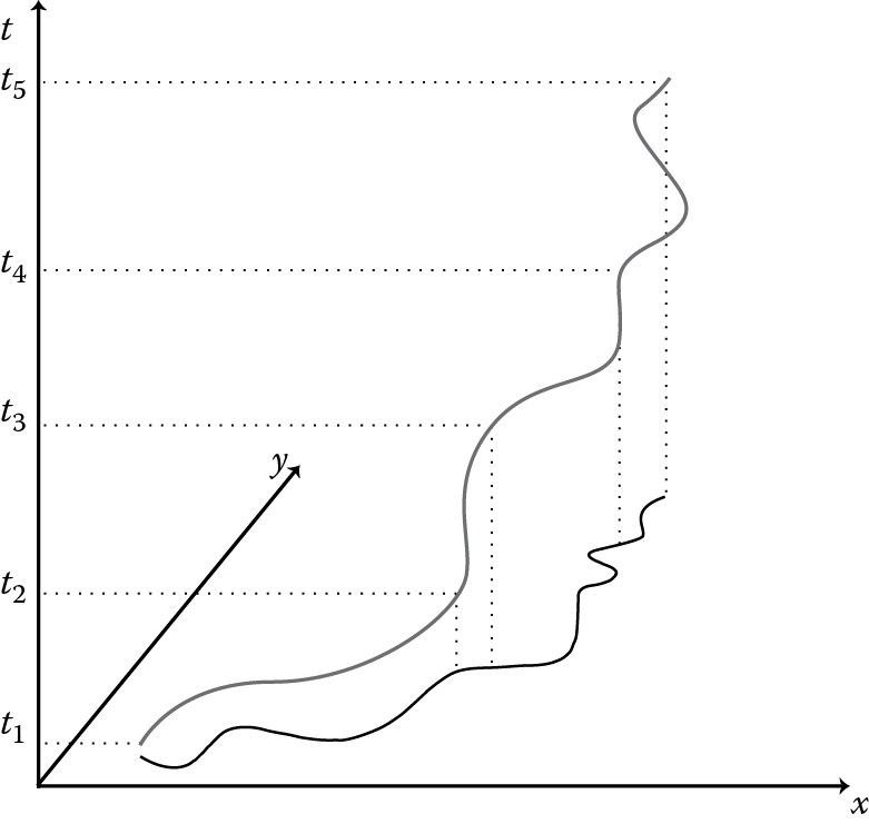
In the sequel, we assume a three-dimensional model for tracing entities (e.g., people, vehicles, commodities, etc.) of known identities that are moving in two spatial and one temporal dimensions. In general, moving objects have spatial extent (i.e., shape), which might be varying over time. Our principal concern is to capture movement characteristics of objects, rather than other changes (appearance, disappearance, etc.) occurring during their lifetime. Without loss of generality, we restrict our interest to point entities (not regions or lines) moving on the Euclidean plane across time, as illustrated in Figure 14.1. As a convention, for a given object id, its successive positional samples p are pairs of geographic coordinates (x, y), measured at discrete, totally ordered timestamps τ from a given time domain. This time domain may be considered as an ordered, infinite set of discrete, primitive time instants (e.g., seconds). Successive positions of an individual object are assigned ever-increasing timestamp values that denote the time at which each recording took place. This time-stamping actually establishes a unique ordering reference among all positional elements. Of course, not all objects may be relaying a new position concurrently. Indeed, sampling rates may not be identical (e.g., a vehicle could report every few seconds, while a pedestrian, once every minute) and may be also varying even for a single object (e.g., less point samples when moving at steady speed along a straight course).
When a large number of objects are being monitored, their relayed time-stamped locations effectively constitute a positional stream of tuples < id, p, τ > that keep arriving into the processing engine from each moving source. However, no deletions or updates are allowed to already-registered locations, so that coherence is preserved among append-only positional items. On the basis of such current locations, the processor may evaluate location-aware queries, for example, detect if a vehicle has just entered into a designated region or if the closest friend has changed. The sequential nature in each object’s path is also very significant in order to inspect movement patterns over a period of time, as well as interactions between objects (e.g., objects traveling together) or with stationary entities (e.g., crossing region boundaries). In essence, this sequence of point locations traces the movement of this object across time. More specifically, trajectory T of a point object identified as id and moving over the Euclidean plane is a possibly unbounded sequence of items consisting of its position p recorded at timestamp τ. Thus, each trajectory is approximated as an evolving sequence of point samples collected from the respective data source at distinct time instants (e.g., a GPS reading taken every few seconds).
Considering that numerous objects may be monitored, this information creates a trajectory stream of locations concurrently evolving in space and time. It is worth mentioning two characteristics inherent in such streaming trajectories. First, time monotonicity dictates a strict ordering of spatial positions taken by a moving object all along its trajectory. Thus, items of the trajectory stream are in increasing temporal order as time advances. Hence, positional tuples referring to the same trajectory can be ordered by simply comparing their time indications. Second, locality in an object’s movement should be expected, assuming that its next location will be recorded somewhere close to the current one. Therefore, it is plausible to anticipate consistent object paths in space, with the possible exception of discontinuities in movement due to communication failures or noise.
Several models and algorithms have been proposed for managing continuously moving objects in spatiotemporal databases. In Reference 13, an abstract data model and a query language were developed toward a foundation for implementing a spatiotemporal Data Base Management System (DBMS) extension where trajectories are considered as moving points. Based on that infrastructure, the SECONDO prototype [14] offered several built-in and extensible operations. Due to obvious limitations in storage and communication bandwidth, it is not computationally efficient to maintain a continuous trace of an object’s movement. As a trade-off between performance and positional accuracy, a discrete model is usually assumed for movement, by simply collecting point samples along its course. The discrete model proposed in Reference 15 decomposes temporal development into fragments and then uses a simple function to represent movement along every such “time slice.” For trajectories, each time slice is a line segment connecting two consecutively recorded locations of a given object, as a trade-off between performance and positional accuracy. In moving-object databases [16], interpolation techniques can be used to estimate intermediate positions between recorded samples and thus approximately reconstruct an acceptable trace of movement. In addition, spline methods have also been suggested as a means to provide synchronized, curve-based trajectory representations by resampling original positional measurements at a fixed rate.
In practice, a trajectory is often reconstructed as a “polyline” vector, that is, a sequence of line segments for each object that connect each observed location to the one immediately preceding it. Therefore, from the original stream of successive positions taken by the moving points, a stream of append-only line segments may be derived online, maintaining progressively the trace of each object’s movement up to its most recent position. Again, no updates are allowed to segments already registered, in order to avoid any modification to historical information and thus preserve coherence among streaming trajectory segments. We adhere to such representation of trajectories as point sequences across time, implying that locations are linearly connected. Also, note that trajectories are viewed from a historical perspective, not dealing at all with predictions about future object positions as in Reference 17. Therefore, robust indexing structures are needed in order to support complex evaluations in both space and time [18].
In LBS applications, several types of location-aware CQs can be expressed, so as to examine spatial interactions among moving objects or with specific static geometries (including spatial containment, range or distance search). According to the classification in Reference 18, two types of spatiotemporal queries can be distinguished:
- Coordinate-based queries. In this case, it is the current position of objects that matters most in typical range [19] and nearest-neighbor search [3].
- Trajectory-based queries, involving the topology of trajectories (topological queries) and derived information, such as speed or heading of objects (navigational queries). Such queries may be used to examine any interactions among trajectories, like joins [8] to identify those that exhibit some kind of similarity (e.g., vehicles following similar routes after 8 a.m.) or nearest-neighbor queries [20]. Clustering operations can also be employed to detect convoys [6], flocks [5], or swarms [21].
In addition, this model conveniently enables calculation of derived attributes, such as speed or acceleration. This information may be produced from location updates after some processing or by simply manipulating time-stamped locations per object. For example, as soon as a positional update is received, the average or instantaneous speed of the respective moving object can be calculated at once. Results may be propagated to a secondary data stream that maintains the speed for each moving object. Note that this kind of derived stream for speed, acceleration, traveled distance, and so forth can be suitably time-stamped with respect to the time indications of incoming tuples, but they do not necessarily retain any spatial features from the original positional stream.
Given that a possibly large but always finite number of location updates arrive for processing at each timestamp τ, the evaluation mechanism must maintain an ordered sequence of all data elements accumulated thus far, practically representing the historical movement of objects. Due to the sheer volume of positional updates and the necessity to answer CQs in real time, it is hardly feasible to deal with lengthy, ever-growing trajectories that represent every detail of the entire history of movement. Instead, it becomes imperative to examine lightweight yet connected motion paths for a limited time period close to the present. Stream processing is mainly achieved by employing CQs, whose results are always refreshed with the most recently arrived positional updates. Such requests usually refer to the most recent portion of objects’ paths, rather than remote ones, since users are primarily concerned with the current or most recent situation. So, they specify evolving periods of interest for their computations (e.g., examine locations received during the last hour), instead of dealing with potentially unbounded object traces piling up during long periods.
This inherent and valuable characteristic, along with time monotonicity, has a subtle effect: After a while, older positions may be considered as obsolete, so they may be either discarded or archived. The semantics of sliding windows [22] against such positional streams are an ideal choice, as trajectories always evolve steadily along the temporal dimension. Such windows actually restrict the amount of inspected data into temporary yet finite chunks. They are declared in user requests against the stream through properties inherent in the data, mostly thanks to timestamps in the incoming items. Typically, users express interest in a recent time range ω (e.g., positions relayed during past 10 min), which gets frequently refreshed every β units (e.g., each minute), so that the window slides forward to keep in pace with newly arriving items. In effect, such windows can naturally abstract the recent portion of trajectories and thus provide synchronized and compact subsequences without temporal gaps.
14.3 Online Trajectory Compression with Spatiotemporal Criteria
One way to deal with the overwhelming volume of streaming positions is to maintain a concise yet quite reliable summary of each object’s movement, avoiding any superfluous details and reducing processing complexity. A suitable algorithm could be based on heuristics, taking advantage of the spatial locality and temporal timeliness that characterize each trajectory, and thus distinguish locations that should be preserved in the compressed paths. As a rule in data stream processing, single-pass algorithms are the most adequate means to effectively summarize massive data items into concise synopses, by examining each incoming point only once. Essentially, there is always a trade-off between approximation quality and both time and space complexity. In the special case of trajectory streams, an additional requirement is posed: Not only exploit the timely spatiotemporal information but also take into account and preserve the sequential nature of the data. Therefore, in order to efficiently maintain trajectories online, there is no other way but to apply compression techniques, thus not only reducing drastically the overall data size but also speeding up query answering, for example, identifying pairs of trajectories that have recently been moving close together. By intelligently dropping some points with negligible influence on the general movement of an object, a simplified yet quite reliable trajectory representation may be obtained. Such a procedure may be used as a filter over the incoming spatiotemporal updates, essentially controlling the stream arrival rate by discarding items before passing them to further processing. Besides, since each object is considered in isolation, such item-at-a-time filtering could be applied directly at the sources, with substantial savings both in communication bandwidth and in computation overhead at the processing engine.
Clearly, there is a need for techniques that can successfully maintain an online summary consisting of the most significant trajectory locations, with minimal process cost per point. Such algorithms should take advantage of the spatiotemporal features that characterize movement, successfully detecting changes in speed and orientation in order to produce a representative synopsis as close as possible to the original route. Our key intuition in the techniques proposed in Reference 23 is that a point should be taken into the sample as long as it reveals a relative change in the course of a trajectory. If the location of an incoming point can be safely predicted (e.g., via interpolation) from the current movement pattern, then this point contributes little information and hence can be discarded without significant loss in accuracy. As a result, retained points may be used to approximately reconstruct the trajectory; discarded locations could be derived via linear interpolation with small error. It is important to note that locations are examined not on the basis of spatial positions only but, rather, on velocity considerations (e.g., speed changes, turns, etc.), such that the sample may catch any significant alterations at the known pattern of movement.
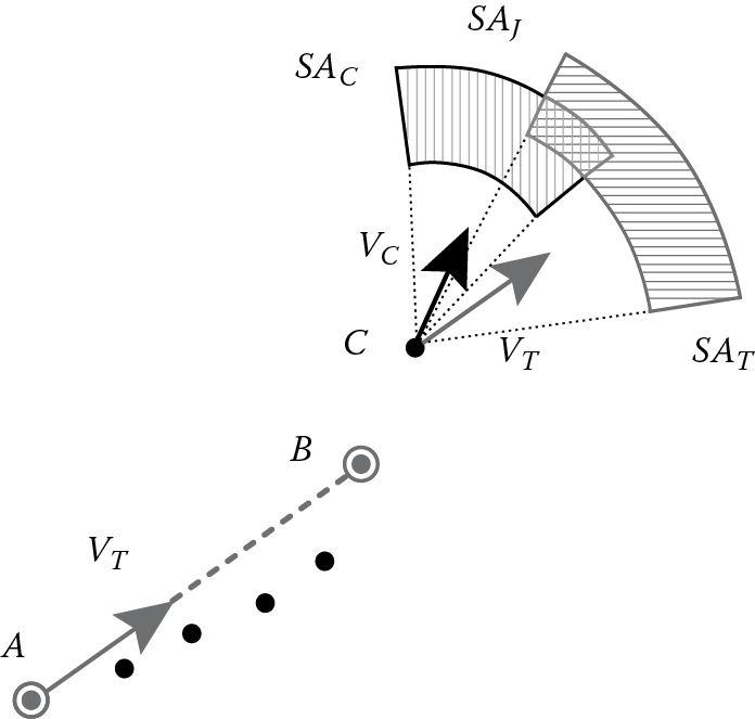
The first algorithm is called threshold-guided sampling because a new point is appended to the retained trajectory sample once a specified threshold is exceeded for an incoming location. A decision to accept or reject a point is taken according to user-defined rules specifying the allowed tolerance (“threshold”) for changes in speed and orientation. In order to decide whether the current location can be safely predicted from the recent past and is thus superfluous, this approach takes under consideration both the mean and instantaneous velocity of the object. As illustrated in Figure 14.2, the mean velocity VT comes from the last two locations (A, B) stored in the current trajectory sample, while the instantaneous velocity VC is derived from the last two observed locations (B, C). Also note that small variations in the orientation of the predicted course are tolerable; hence, deviation by a few degrees is allowed, as long as it does not change the overall direction of movement by more than dϕ (threshold parameter in degrees). Actually, the corresponding two loci derived by these criteria are the ring sections SAT and SAC, called “safe areas,” where the object is normally expected to be found next, according to the mean and current instantaneous velocities, respectively. As justified in Reference 23, it is not sufficient to use only one of these loci as a criterion to drop locations, because critical points may be missed and errors may be propagated and hence lead to distortions in the compressed trajectories. Instead, taking the intersection SAJ of the two loci shown in Figure 14.2 as a joint safe area is a more secure policy. As time goes by, this area is more likely to shrink as the number of discarded points increases after the last insertion into the sample, so the probability of missing any critical points is diminishing. As soon as no intersection of these loci is found, an insertion will be prompted into the compressed trajectory, regardless of the current object location. The only problem with this scheme is that the total amount of items in the trajectory sample keeps increasing without eliminating any point already stored, so it is not possible to accommodate under a fixed memory space allocated to each trajectory.
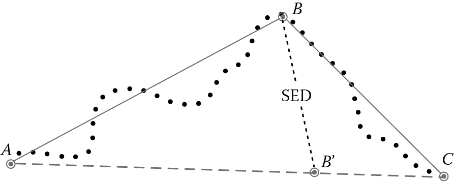
To remedy this downside, the second algorithm introduced in Reference 23 and called STTrace is more tailored for streaming environments. The intuition behind STTrace is to use an insertion scheme based on the recent movement features but at the same time allowing deletions from the sample to make room for the newly inserted points without exceeding allocated memory per trajectory. However, a point candidate for deletion is chosen not randomly over the current sample contents but according to its significance in trajectory preservation. In order to quantify the importance of each point in the trajectory, we used a metric based on the notion of synchronous Euclidean distance (SED) [24]. As shown in Figure 14.3, for any point B in the retained sample (i.e., the compressed trajectory), SED is the distance between its actual location and its time-aligned position B’ estimated via interpolation between its predecessor A and successor point C in the sample. Since this is essentially the distance between the actual point and its spatiotemporal trace along the line segment that connects its immediate neighbors in the sequence, this sampling algorithm was named STTrace. Admittedly, it is better to discard a point that will produce the least distortion to the current trajectory synopsis. As soon as the allocated memory gets exhausted and a new point is examined for possible insertion, the compressed representation is searched for the item with the lowest SED. That point represents the least possible loss of information in case it gets discarded. But this comes at a cost: For every new insertion, the most appropriate candidate point must be searched for deletion over the entire sample with O(N) worst-case cost, where N is the actual size of the compressed trajectory. Nevertheless, as N is expectedly very small and the sampled points may be maintained in an appropriate data structure (e.g., a binary balanced tree) with logarithmic cost for operations (search, insert, delete), normally, this is an affordable trade-off.
There have been several other attempts to compress moving-object traces, either through load shedding policies on incoming locations like in References 25 through 27 or by taking also into account trajectory information as in References 28 and 29. Still, based on a series of experiments reported in Reference 23, threshold-guided sampling emerges as a robust mechanism for semantic load shedding for trajectories, filtering out negligible locations with minor computational overhead. The actual size of the sample it provides is a rough indication of the complexity of each trajectory, and the parameters can be fine-tuned according to trajectory characteristics and memory availability. Besides, it can be applied close to the data sources instead of a central processor, sparing both transmission cost and processing power. Regarding efficiency, STTrace always manages to maintain a small representative sample for a trajectory of unknown size. It outperforms threshold-guided sampling for small compression rates since it is not easy to define suitable threshold values in this case. Empirical results show that STTrace incurs some overhead in maintaining the minimum synchronous distance and in-memory adjustment of the sampled points. However, this cost can be reduced if STTrace is applied in a batch mode, that is, executed at consecutive time intervals.
14.4 Amnesic Multiresolution Trajectory Synopses
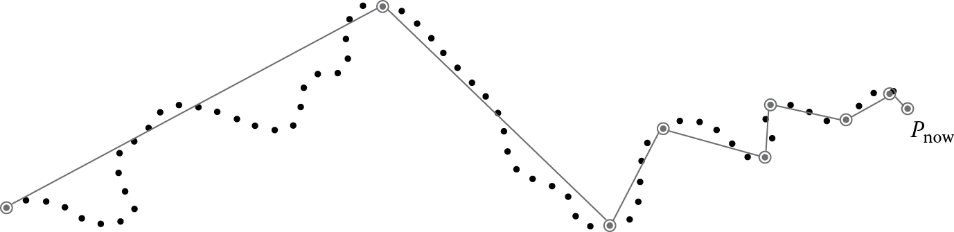
It is apparent that the significance of each isolated location is inherently time decaying, since any recorded position of an object will be soon outdated by forthcoming ones. This motivates a policy for dropping detail with age: The older a location gets, the coarser its representation could become in a progressive fashion, implying that greater precision should be reserved for the most recent positions, as exemplified in Figure 14.4. Effectively, this amnesic treatment of trajectories can cope with the frequent positional updates gathered per object, known as the velocity challenge in big trajectory data.
With respect to approximation of one-dimensional time series, a wide range of amnesic functions was identified in Reference 30, useful in controlling the amount of error tolerated for every single point in the time series. In our work in Reference 31, we presented a multiple-granularity framework based on an amnesic tree structure (AmTree), which accepts streaming items and maintains summaries over hierarchically organized levels of precision, essentially realizing an amnesic behavior over stream portions. In addition, different levels of abstraction are inherent in semantics related to multiscale representation of spatiotemporal features, allowing progressive refinements of their evolution. This time-aware scheme distantly resembles SWAT [32], but this latter is intrinsically bound to wavelet transform of scalar stream values and cannot handle multidimensional points with user-specified approximation functions.
Actually, AmTree can be easily calibrated to work with a varying number of time granules (i.e., nodes) per level. In Figure 14.5, we present several consecutive snapshots of this amnesic processing scheme that manipulates pairs of items at every level. For simplicity, we utilize one-dimensional numeric values and not two-dimensional positional ones, and we assume that a time granule at each level spans two granules half its temporal span at the level beneath. Except for the root, each level i of the tree consists of a right (Ri) and a left node (Li). At the lowest level, node R0 accepts data with reference to the finest time granularity (e.g., seconds), which characterizes every timestamp attached to incoming tuples. Each node at level i contains information across twice as many timestamps as a node at level i − 1. Hence, a node at level i contains information characterizing 2i timestamps, and it is being updated accordingly.
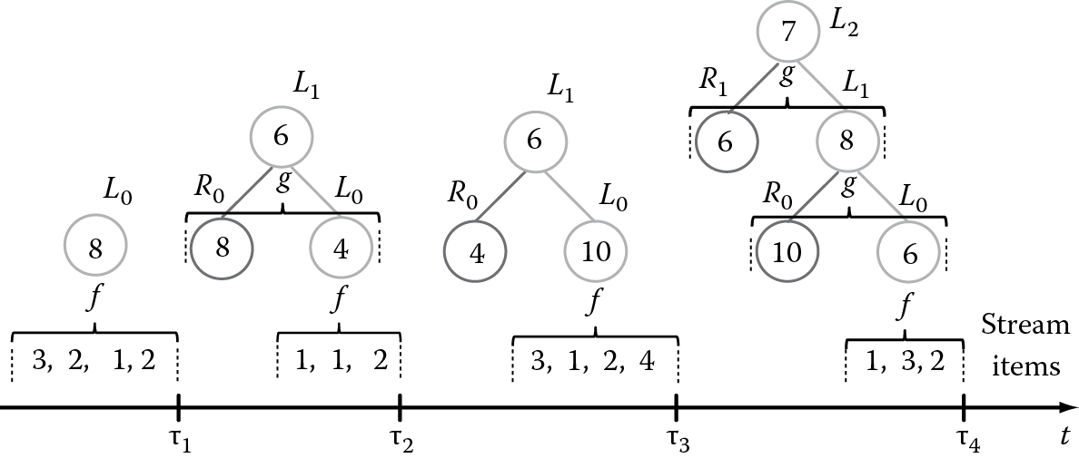
Once this structure starts consuming streaming items, node updates are performed in a bottom-up fashion. A user-defined mapping f is applied over the batch of fresh positions with current timestamp value τ and transforms them into a single tuple that can become the content of a tree node. As illustrated in Figure 14.5, where f is a simple summation of numeric items, the resulting content is assigned to node R0, while the previous content of R0 is shifted to node L0. As time goes by and new data come in, the contents of each level are merged using a function g (average in the example of Figure 14.5) and propagated higher up in the tree, thus retaining less detail. Note that node R0 is the only entry point to the synopsis maintained by the AmTree. As justified in Reference 31, AmTree updates can be carried out online in O(1) amortized time per location with only logarithmic requirements in memory storage.
This framework is best suited for summarizing streams of sequential features, and it has been applied to create amnesic synopses concerning singleton trajectories. As an alternative representation to a time series of points, the trajectory of a moving object can be represented with a polyline composed of consecutive displacements. Every such line segment connects a pair of successive point locations recorded for this object, eventually providing a continuous, though approximate, trace of its movement. With respect to compressing a single trajectory, an AmTree instantiation manipulates all successive displacement tuples relayed by this object. In direct correspondence to the generic AmTree functionality, mapping f converts every current object position into a displacement tuple with respect to its previous location. This displacement is then inserted into the R0 node, possibly triggering further updates higher up in the AmTree. When the contents of level i must be merged to produce a coarser representation, a simple concatenation function g is used to combine the successive displacements stored in nodes Li and Ri. After eliminating the common articulation point of the two original segments, a single line segment is produced and then stored in node Ri+1. As a result, end points of all displacements stored in AmTree nodes correspond to original positional updates, while consecutive displacements remain connected to each other at every level. Evidently, an amnesic behavior is achieved for trajectory segments through levels of gradually less detail in this bottom-up tree maintenance. As long as successive displacements are preserved, the movement of a particular object can be properly reconstructed by choosing points in descending temporal order, starting from its most recent position and going steadily backward in time. Any trajectory reconstruction process can be gradually refined by combining information from multiple levels and nodes of the tree, leading to a multiresolution approximation for a given trajectory, as depicted in Figure 14.4.
This structure can also provide unbiased estimates for the number of objects that are moving in an area of interest during a specified time interval. When each object must be counted only once, the problem is known as distinct counting [33]. We consider a regular decomposition of the two-dimensional Euclidean plane into equal-area grid cells, which serve as a simplified spatial reference for the moving objects instead of their exact coordinates. Thus, each cell corresponds to a separate AmTree, which maintains gradually aging information concerning the number of moving objects inside that cell. Query-oriented compression is achieved using Flajolet-Martin (FM) sketches [34], which are based on Probabilistic Counting with Stochastic Averaging (FM_PCSA). Each node of an AmTree retains m bitmap vectors utilized by the FM_PCSA sketch, as illustrated in Figure 14.6. Hence, we avoid enumeration of objects, as we are satisfied with an acceptable estimate of their distinct count (DC) given by the sketching algorithm. In order to estimate the number of distinct objects moving within a given area a during a time interval Δτ, we first identify the grid cells that completely cover region a. Those cells determine the group of qualifying AmTree structures that maintain the aggregates. For each such tree, we need to locate the set of nodes that overlap time period Δτ specified by the query; these nodes are identical for each qualifying tree. By taking the union of the sketches attached to these nodes (i.e., an OR operation over the respective bitmaps), we can finally provide an approximate answer to the DC query.
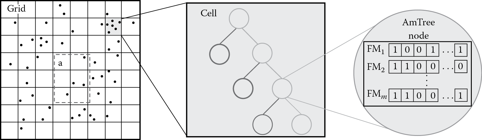
The three-tier FM-AmTree structure used for approximate distinct counting of moving objects.
The experimental study conducted in Reference 31 confirms that recent trajectory segments always remain more accurate, while overall error largely depends on the temporal extent of the query in the past. Even for heavily compressed trajectories, accuracy is proven quite satisfactory for answering spatiotemporal range queries. With respect to DC queries, it was observed that a finer grid partitioning incurs more processing time at the expense of increased accuracy.
Overall, the suggested AmTree framework is a modular amnesic structure with exponential decay characteristics. It is especially tailored to cope with streaming positional updates, and it can retain a compressed outline of entire trajectories, always preserving contiguity among successive segments for each individual object. Effectively, such a policy constructs a multiresolution path, offering finer motion paths for the recent past and keeping gradually less and less details for aging parts of the trajectory.
In conjunction with FM sketches, AmTree can further be used in spatiotemporal aggregation for providing good-quality estimates to DC queries over locations of moving objects.
14.5 Continuous Range Search over Uncertain Locations
Recently, the increasingly popular social networking applications have been enhanced with location-aware features toward geosocial networking services [35], thus allowing mobile users to interact relative to their current positions. Platforms like Facebook Places [36], Google Latitude [37], and Foursquare [38] enable users to pinpoint friends on a map and share their whereabouts and preferences with the followers they choose. Despite their attraction, such features may put people’s privacy at risk, revealing sensitive information about everyday habits, political affiliations, cultural interests, and so forth. Mobile users are aware of their own exact location, but they may not wish to disclose it to third parties; instead, they consent to relay just a cloaked indication of their whereabouts [39]; hence, the veracity of this information is purposely limited.
In Reference 40, we suggested a framework for real-time processing of continuous range queries against such imprecise locations, so that a user may receive instant notifications when a friend appears with sufficient probability within his/her area of interest (e.g., “it is more than 75% probable that one of my friends is in my neighborhood”). Each position is obfuscated as an uncertainty region ro with bivariate Gaussian characteristics, enclosing (but apparently not centered at) the user’s current location. Depending on the variance, the density of a Gaussian random variable is rapidly diminishing with increasing distances from the mean. Thanks to its inherent simplicity, the uncertainty region can be truncated in a natural way on the server side, so the user itself does not need to specify a bounded area explicitly. It suffices that an object sends the origin (μx, μy) of its own probability density function (pdf) and the standard deviation σ (common along both spatial dimensions). As illustrated in Figure 14.7a, there is 99.73% probability that the actual location is found somewhere within a radius 3σ from the origin. Uncertainty parameters are expressed in distance units (e.g., meters) and can be changed dynamically as the object is moving or adjusting its degree of privacy. Larger σ values indicate that an object’s location can be hidden in a greater area around its indicated mean (μx, μy). Based on such massive, transient, imprecise data, the server attempts to give a response to multiple search requests. Each CQ q may dynamically modify its spatial range (a moving rectangular extent rq) and its cutoff probability threshold θ. Evaluation takes place periodically at execution cycles, upon reception of a batch of updates from objects and changes in queries. Query q identifies any object o registered as a member in its contact list Lq (e.g., friends or followers of q) and is currently within range rq with an appearance probability of at least θ.
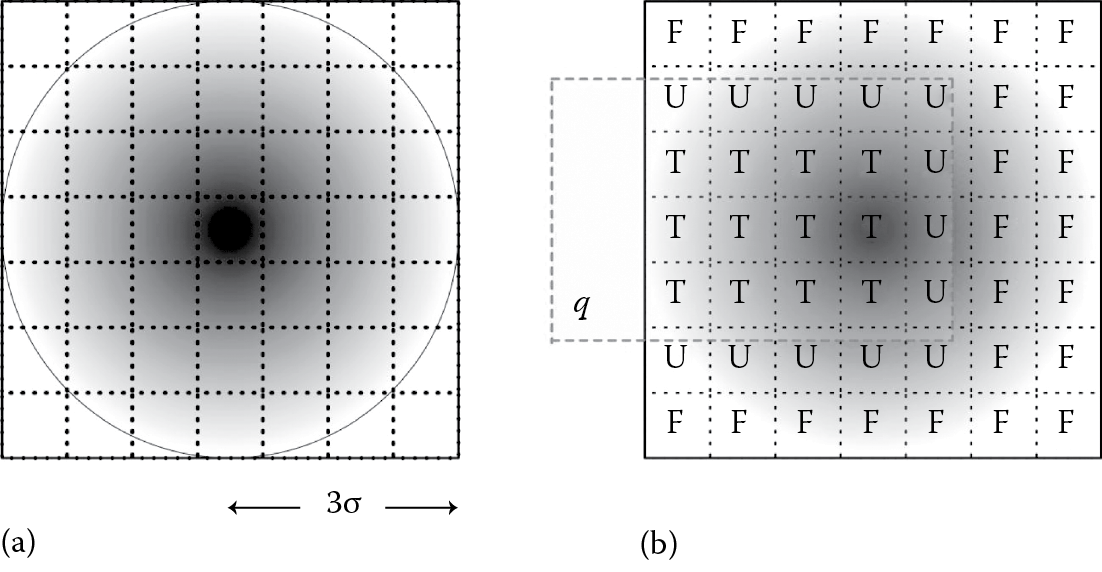
(a) Standard bivariate Gaussian distribution N(0, 1) as a model for an uncertain location. (b) Verifier with 7 × 7 elementary boxes for checking an object against range query q.
The problem is that Gaussian distributions cannot be integrated analytically, whereas numerical methods like Monte Carlo are prohibitively costly for getting a fair estimation for appearance probabilities in online fashion. Given the mobility and mutability of objects and queries alike, in Reference 40, we approximated each uncertainty region with its rectilinear circumscribed square of side 6σ around the origin of the pdf. As illustrated in Figure 14.7a, the cumulative probability of this minimum bounding box (MBB) is greater than 99.73% and tends asymptotically to 1, although its area is larger than the circle of radius 3σ. If this MBB were uniformly subdivided into λ × λ elementary boxes, then each box would represent diverse cumulative probabilities, indicated by the differing shades in Figure 14.7a. However, for a known σ, the cumulative probability in each elementary box is independent of the parameters of the applied bivariate Gaussian distribution. Once precomputed (e.g., by Monte Carlo), these probabilities can be retained in a lookup table.
The rationale behind this subdivision is that it may be used as a discretized verifier V when probing uncertain Gaussians. Consider the case of query q against an object, shown as a shaded rectangle in Figure 14.7b. Depending on its topological relation with the given query, each elementary box of V can be easily characterized by one of three possible states: (1) T is assigned to elementary boxes totally within query range; (2) F signifies disjoint boxes, that is, those entirely outside the range; and (3) U marks boxes partially overlapping with the specified query range. Then, summing up the respective cumulative probabilities for each subset of boxes returns three indicators pT , pF, and pU suitable for object validation against the cutoff threshold θ. The confidence margin in the results equals the overall cumulative probability of the U-boxes, which depends entirely on granularity λ. Indeed, a small λ can provide answers quickly, which is critical when coping with numerous objects. In contrast, the finer the subdivision into elementary boxes (i.e., a larger λ), the less the uncertainty in the emitted results.
As a trade-off between timeliness and answer quality in a geostreaming context, in Reference 40, we turned this range search into an (ε, δ) approximation problem, where ε quantifies the error margin in the allowed overestimation when reporting a qualifying object and δ specifies the tolerance that an invalid answer may be given (i.e., a false positive). We introduced several optimizations based on inherent probabilistic and spatial properties of the uncertain streaming data; details can be found in Reference 40.
In a nutshell, this technique can quickly determine whether an item possibly qualifies for the query or safely prune examination of nonqualifying cases altogether. Inevitably, such a probabilistic treatment returns approximate answers, along with confidence margins as a measure of their quality. Simulations over large synthetic data sets indicated that, compared with an exhaustive Monte Carlo evaluation, about 15% of candidates were eagerly rejected, while another 25% were pruned. Most importantly, false negatives were less than 0.1% in all cases, which demonstrates the efficiency of this approach. Qualitative results are similar for varying λ, but finer subdivisions naturally incur increasing execution costs, yet always at least an order of magnitude more affordable than naïve Monte Carlo evaluation.
14.6 Multiplexing of Evolving Trajectories
Identifying objects that approximately travel together over a recent time interval would also be important for reducing storage requirements as well as in fast query answering when dealing with big trajectory data. Our work in Reference 41 suggests a framework that intends to cope with the great variety of paths being monitored in applications that handle massive motion data, as in traffic monitoring (e.g., carpooling services); fleet management (logistics); airspace control using radars; biodiversity protection (e.g., for tracking wildlife); and so forth. The key idea is that a symbolic encoding for sequences of trajectory segments may offer a rough yet succinct abstraction of their concurrent evolution. Intuitively, a processing scheme could take advantage of inherent spatiotemporal properties, such as heading, speed, and current position, in order to continuously report groups of objects with similar motion traces. Then, an indicative “delegate” path could be regularly constructed per detected group, since it could actually epitomize spatiotemporal features shared by its participating objects.
The main objective of this scheme is to detect groups of objects according to the following constraints:
- Similarity: pairwise similar trajectory segments must be within distance ε.
- Simultaneity: positions are checked over a recent sliding window [22] with temporal range ω.
- Timeliness: groups are adjusted periodically every β time units (i.e., once the window slides), in order to reflect any changes in objects’ movement.
Hence, pairs of concurrently recorded locations from each object should not deviate more than ε during interval ω. This notion of similarity is confined within the recent past (window ω) and does not extend over the entire history of movement. Moreover, it can be easily generalized for multiple objects with pairwise similar trajectory segments (Figure 14.8). In addition, a threshold is applied when incrementally creating “delegate” traces from such trajectory groupings; a synthetic trace T is returned only if the respective group currently includes more than n objects. Note that no original location in such a group can deviate more than the given tolerance ε from its delegate path T.
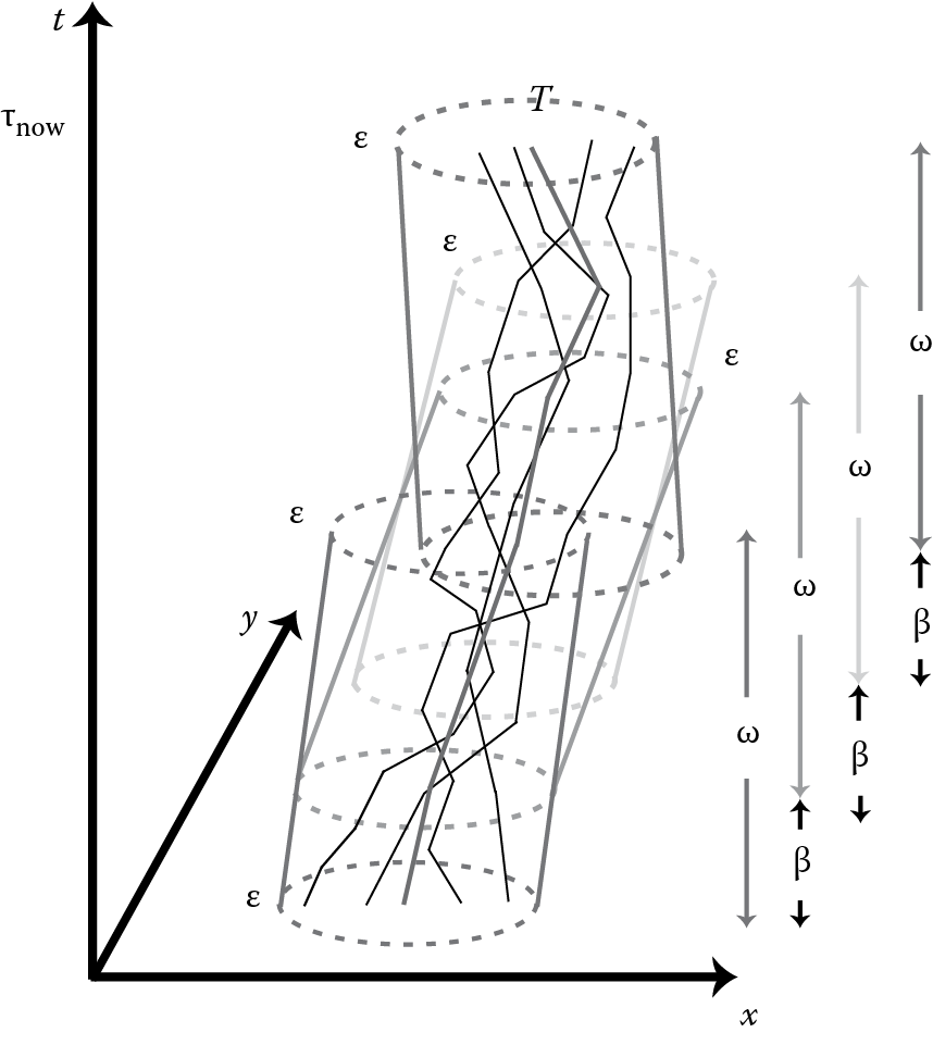
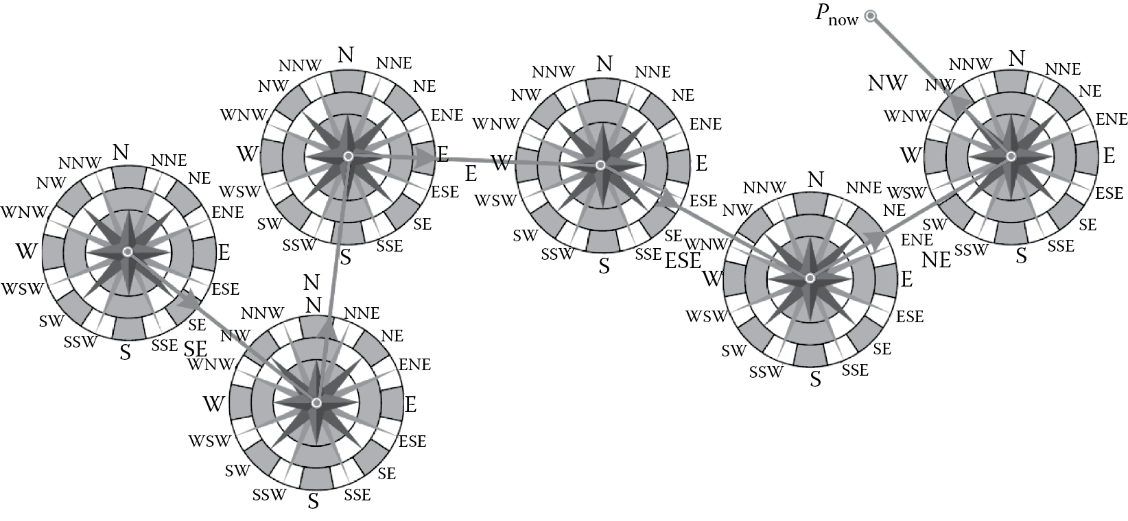
Checking the similarity of trajectory segments according to their time-stamped positions soon becomes a bottleneck for escalating numbers of moving objects or wider window ranges. To avoid this, in Reference 41, we opt for an approximate representation of traces based on consecutive velocity vectors that end up at the current location of each respective object (Figure 14.9). Every vector is characterized by a symbol that signifies the orientation of movement using the familiar notion of a compass, which roughly exemplifies an object’s course between successive position messages. Effectively, compass resolution α determines the degree of motion smoothing; when α = 4, orientation symbols {N, S, E, W} offer just a coarse indication, but finer representations are possible with α = 16 symbols (Figure 14.9) or more. Typically, once the window slides at the next execution cycle, an additional symbol (approximating motion during the latest β timestamps) will be appended at the tail of this first-in, first-out (FIFO) sequence, while the oldest one (i.e., at the head) gets discarded. Thus, instead of the bulk of original positions, only a series of few symbols and speed measures need be maintained per trajectory, thus offering substantial memory savings.
Symbolic sequences are more amenable to similarity checks since they act as motion signatures. In Reference 41, we identified objects with common signatures through a hash table. Objects with identical symbolic sequences might have almost “parallel” courses but can actually be very distant from each other. The crux of our approach is that objects with identical signatures and currently within distance ε from each other most probably have followed similar paths recently. Therefore, identifying groups of at least n objects with a common signature can be performed against their current locations through a point clustering technique. We provisionally make use of the Density-Based Spatial Clustering of Applications with Noise (DBSCAN) algorithm [42] to detect groups of similar trajectories with proximal current positions. Afterward, a delegate path T per discovered cluster with sufficient membership (>n objects) can be easily created by simply starting from the most recent location and rewinding the symbolic sequence backward, that is, reversely visiting all samples retained within the sliding window frame.
Simulations against synthetic trajectories have shown that this framework has great potential for data reduction and timely detection of motion trends, without hurting performance or approximation quality. Some preliminary results regarding traffic trends on the road network of Athens are available in Reference 41.
Overall, we believe that this ongoing work fuses ideas from trajectory clustering [7] and path simplification [23] but proceeds further beyond. Operating in a geostreaming context, not only can it identify important motion patterns in online fashion, but it may also provide concise summaries without resorting to sophisticated spatiotemporal indexing. Symbolic representation of routes was first proposed in Reference 8 for filtering against trajectory databases. Yet, our encoding differs substantially, as it attempts to capture evolving spatiotemporal vectors using a versatile alphabet of tunable object headings instead of simply compiling time-stamped positions in a discretized space. In practice, processed features may serve various needs, such as the following: (i) data compression, by collectively representing traces of multiple objects with a single “delegate” that suitably approximates their common recent movement; (ii) data discovery, by detecting trends or motion patterns from real-time location feeds; (iii) data visualization, by estimating the significance of each multiplexed group of trajectories and illustrating its mutability across time; and (iv) query processing, if multiplexed traces are utilized at the filtering stage when evaluating diverse queries (range, k-NN, aggregates, etc.) instead of the detailed, bulky trajectories.
14.7 Toward Next-Generation Management of Big Trajectory Data
Processing trajectory data sets with a focus on their inherent spatiotemporal features has been widely studied in the last decade. However, big spatiotemporal data brings in new research challenges and the need for effective and efficient ways to process such information and extract useful knowledge.
Undoubtedly, the processing infrastructure should be able to tackle scalability and load balancing. Stream processing in the cloud may offer flexible, highly distributed resource allocation, as data emanates from multimodal devices and flows through heterogeneous networks. For instance, Hadoop-GIS [43] is a scalable and high-performance data warehousing system specifically for spatial data and queries. Running on Hadoop, it supports several types of queries (including spatial join, containment, aggregation, etc.) through partitioning and multilevel spatial indexing.
Novel index structures are also needed to support a variety of queries regarding spatial proximity, navigation, recommendation, and so forth, as well as interaction with trajectories. TrajStore [44] is a recently proposed scheme for indexing, clustering, and storing trajectory data, which is optimized for retrieving data about many trajectories passing through a particular location. The suggested index dynamically identifies both spatially and temporally adjacent segments in order to compress them on disk.
Exploring dynamic motion patterns across time, like flocks [5], convoys [6], traveling companions [45], or swarms [21], is a very attractive topic and may have many applications, for example, in fleet management, carpooling services, biodiversity protection, and so forth. These concepts aim to identify groups of moving objects traveling together for a certain time period. The recent notion of gathering [46] is able to model a variety of additional group events or incidents. Examples include celebrations, parades, large-scale business promotions, protests, traffic jams, and other public congregations.
Regarding more specific analytics, the methodology in Reference 47 identifies time period–based most-frequent paths over large trajectory data sets. The proposed two-step strategy first constructs a graph with the frequencies of the candidate paths and then executes a graph search to find the results. The SimpleFleet platform [48] aggregates online data from vehicle trajectories and provides live traffic analytics for large metropolitan areas, including services for route searching; statistics; as well as map visualization of paths, traffic conditions, and isochrones. This may be useful in car navigation, in order to recommend routes according to actual traffic patterns. vTrack [49] is a prototype system that uses mobile phones in order to accurately estimate road travel times from a sequence of inaccurate position samples. For example, if GPS readings are unavailable or erroneous (e.g., in “urban canyons”), it is possible to use alternative, but noisier, sensors (like Wi-Fi) so as to estimate both a user’s trajectory and travel times. The techniques proposed in Reference 50 are based on a multicost, time-dependent, uncertain graph model of a road network according to GPS positions from vehicles. Thus, optimal routes may consider multiple costs and time-dependent uncertainty for a given origin–destination pair and a start time.
Rapid proliferation of popular, location-based social networking (e.g., Foursquare, Facebook) has also given rise to large amounts of trajectories associated with activity information. Such activity trajectories [51] essentially record not only the spatiotemporal aspects of movement but textual descriptions of users’ activities as well. This gives rise to interesting problems such as similarity retrieval: Given a sequence of query locations, each associated with a set of desired activities, an activity trajectory similarity query returns k trajectories that cover the query activities and yield the shortest minimum match distance [51]. It is expected that more interesting problems around spatiotextual descriptions of activities in time will emerge, including personalized aspects of similarity retrieval [52].
Similarly, interpreting human lifestyles [53] not only is essential to many scientific disciplines but also has a profound business impact on geomarketing applications. Devising algorithms that integrate data from multiple social network accounts of millions of individuals along with their publicly available heterogeneous behavioral data as stored in location-based social networks could lead to interesting classification schemes. The results can be precious for personalized recommendation and targeted advertising.
Another increasingly common trend is the advent of geographic information created by voluntary communities, known as volunteered geographic information (VGI) or crowdsourced geospatial data [54]. The OpenStreetMap project [55] is one of the most successful VGI efforts, which aims to develop a collaborative, freely available, digital map of the planet with contributions from volunteers. Another form of crowdsourcing is location sharing in social media, such as annotated Twitter posts [56] or geo-tagged photos in Flickr [57]. Beyond issues in privacy [58], extra processing is required on these social media data to retrieve any spatial information [59]. Due to the nonauthoritative nature, VGI efforts have often been questioned regarding the quality and reliability of the information collected. Preprocessing and noise removal of VGI seems a promising research direction toward addressing uncertainty in these spatiotemporal data.
Last, but not least, next-generation platforms should offer advanced functionality to users in order to better deal with the peculiarities in trajectory data and better interpret hidden properties. Interactive mapping tools should sustain the bulk of data, by leveraging representation detail according to the actual map scale, the amount of distinct objects, the complexity of their traces, and so forth. In application development, APIs for fine-grain control over complex events that could correlate dynamic positional data against stationary data sets (e.g., transportation networks or administrative boundaries) or other trajectories would be valuable as well. Finally, dealing with inherent stream imperfections like disorder or noise would offer the ability for dynamic revision of query results, thus increasing the quality of answers.
References
1. Agrawal, D., P. Bernstein, E. Bertino, S. Davidson, U. Dayal, M. Franklin, J. Gehrke, L. Haas, A. Halevy, J. Han, H.V. Jagadish, A. Labrinidis, S. Madden, Y. Papakonstantinou, J.M. Patel, R. Ramakrishnan, K. Ross, C. Shahabi, D. Suciu, S. Vaithyanathan, and J. Widom. 2012. Challenges and Opportunities with Big Data—A Community White Paper Developed by Leading Researchers across the United States. Available at http://www.cra.org/ccc/files/docs/init/bigdatawhitepaper.pdf (accessed April 30, 2014).
2. Stonebraker, M., U. Cetintemel, and S. Zdonik. 2005. The 8 Requirements of Real-Time Stream Processing. ACM SIGMOD Record, 34(4):42–47.
3. Mouratidis, K., M. Hadjieleftheriou, and D. Papadias. 2005. Conceptual Partitioning: An Efficient Method for Continuous Nearest Neighbor Monitoring. In Proceedings of the 24th ACM SIGMOD International Conference on Management of Data, pp. 634–645.
4. Hu, H., J. Xu, and D.L. Lee. 2005. A Generic Framework for Monitoring Continuous Spatial Queries over Moving Objects. In Proceedings of the 24th ACM SIGMOD International Conference on Management of Data, pp. 479–490.
5. Vieira, M., P. Bakalov, and V.J. Tsotras. 2009. On-line Discovery of Flock Patterns in Spatio-Temporal Data. In Proceedings of the 17th ACM SIGSPATIAL International Conference on Advances in Geographic Information Systems (ACM GIS), pp. 286–295.
6. Jeungy, H., M.L. Yiu, X. Zhou, C.S. Jensen, and H.T. Shen. 2008. Discovery of Convoys in Trajectory Databases. Proceedings of Very Large Data Bases (PVLDB), 1(1):1068–1080.
7. Lee, J., J. Han, and K. Whang. 2007. Trajectory Clustering: A Partition-and-Group Framework. In Proceedings of the 26th ACM SIGMOD International Conference on Management of Data, pp. 593–604.
8. Bakalov, P., M. Hadjieleftheriou, E. Keogh, and V.J. Tsotras. 2005. Efficient Trajectory Joins Using Symbolic Representations. In MDM, pp. 86–93.
9. Chen, Z., H.T. Shen, and X. Zhou. 2011. Discovering Popular Routes from Trajectories. In Proceedings of the 27th International Conference on Data Engineering (ICDE), pp. 900–911.
10. Sacharidis, D., K. Patroumpas, M. Terrovitis, V. Kantere, M. Potamias, K. Mouratidis, and T. Sellis. 2008. Online Discovery of Hot Motion Paths. In Proceedings of the 11th International Conference on Extending Database Technology (EDBT), pp. 392–403.
11. Manyika, J., M. Chui, B. Brown, J. Bughin, R. Dobbs, C. Roxburgh, and A.H. Byers. 2011. Big Data: The Next Frontier for Innovation, Competition, and Productivity. McKinsey Global Institute, New York. Available at http://www.mckinsey.com/insights/business_technology/big_data_the_next_frontier_for_innovation (accessed April 30, 2014).
12. Ferguson, M. 2012. Architecting a Big Data Platform for Analytics. Whitepaper Prepared for IBM.
13. Güting, R.H., M.H. Böhlen, M. Erwig, C.S. Jensen, N.A. Lorentzos, M. Schneider, and M. Vazirgiannis. 2000. A Foundation for Representing and Querying Moving Objects. ACM Transactions on Database Systems, 25(1):1–42.
14. Güting, R.H., T. Behr, and C. Duentgen. 2010. SECONDO: A Platform for Moving Objects Database Research and for Publishing and Integrating Research Implementations. IEEE Data Engineering Bulletin, 33(2):56–63.
15. Forlizzi, L., R.H. Güting, E. Nardelli, and M. Schneider. 2000. A Data Model and Data Structures for Moving Objects Databases. In Proceedings of the 19th ACM SIGMOD International Conference on Management of Data, pp. 319–330.
16. Pfoser, D., and C.S. Jensen. 1999. Capturing the Uncertainty of Moving-Object Representations. In Proceedings of the 6th International Symposium on Advances in Spatial Databases (SSD), pp. 111–132.
17. Sistla, A.P., O. Wolfson, S. Chamberlain, and S. Dao. 1997. Modeling and Querying Moving Objects. In Proceedings of the 13th International Conference on Data Engineering (ICDE), pp. 422–432.
18. Pfoser, D., C.S. Jensen, and Y. Theodoridis. 2000. Novel Approaches to the Indexing of Moving Object Trajectories. In Proceedings of 26th International Conference on Very Large Data Bases (VLDB), pp. 395–406.
19. Mokbel, M., X. Xiong, and W. Aref. 2004. SINA: Scalable Incremental Processing of Continuous Queries in Spatiotemporal Databases. In Proceedings of the 23rd ACM SIGMOD International Conference on Management of Data, pp. 623–634.
20. Frentzos, E., K. Gratsias, N. Pelekis, and Y. Theodoridis. 2007. Algorithms for Nearest Neighbor Search on Moving Object Trajectories. GeoInformatica, 11(2):159–193.
21. Zhenhui, L., D. Bolin, H. Jiawei, and R. Kays. 2010. Swarm: Mining Relaxed Temporal Moving Object Clusters. Proceedings on Very Large Data Bases (PVLDB), 3(1–2):723–734.
22. Patroumpas, K., and T. Sellis. 2011. Maintaining Consistent Results of Continuous Queries under Diverse Window Specifications. Information Systems, 36(1):42–61.
23. Potamias, M., K. Patroumpas, and T. Sellis. 2006. Sampling Trajectory Streams with Spatiotemporal Criteria. In Proceedings of the 18th International Conference on Scientific and Statistical Data (SSDBM), pp. 275–284.
24. Meratnia, N., and R. de By. 2004. Spatiotemporal Compression Techniques for Moving Point Objects. In Proceedings of the 9th International Conference on Extending Database Technology (EDBT), pp. 765–782.
25. Nehme, R., and E. Rundensteiner. 2007. ClusterSheddy: Load Shedding Using Moving Clusters over Spatio-Temporal Data Streams. In Proceedings of the 12th International Conference on Database Systems for Advanced Applications (DASFAA), pp. 637–651.
26. Gedik, B., L. Liu, K. Wu, and P.S. Yu. 2007. Lira: Lightweight, Region-Aware Load Shedding in Mobile CQ Systems. In Proceedings of the 23rd International Conference on Data Engineering (ICDE), pp. 286–295.
27. Mokbel, M.F., and W.G. Aref. 2008. SOLE: Scalable On-line Execution of Continuous Queries on Spatio-Temporal Data Streams. VLDB Journal, 17(5):971–995.
28. Cao, H., O. Wolfson, and G. Trajcevski. 2006. Spatio-Temporal Data Reduction with Deterministic Error Bounds. VLDB Journal, 15(3):211–228.
29. Lange, R., F. Dürr, and K. Rothermel. 2011. Efficient Real-Time Trajectory Tracking. VLDB Journal, 25:671–694.
30. Palpanas, T., M. Vlachos, E. Keogh, D. Gunopulos, and W. Truppel. 2004. Online Amnesic Approximation of Streaming Time Series. In Proceedings of the 20th International Conference on Data Engineering (ICDE), pp. 338–349.
31. Potamias, M., K. Patroumpas, and T. Sellis. 2007. Online Amnesic Summarization of Streaming Locations. In Proceedings of the 10th International Symposium on Spatial and Temporal Databases (SSTD), pp. 148–165.
32. Bulut, A., and A.K. Singh. 2003. SWAT: Hierarchical Stream Summarization in Large Networks. In Proceedings of the 19th International Conference on Data Engineering (ICDE), pp. 303–314.
33. Tao, Y., G. Kollios, J. Considine, F. Li, and D. Papadias. 2004. Spatio-Temporal Aggregation Using Sketches. In Proceedings of the 20th International Conference on Data Engineering (ICDE), pp. 214–226.
34. Flajolet, P., and G.N. Martin. 1985. Probabilistic Counting Algorithms for Database Applications. Journal of Computer and Systems Sciences, 31(2):182–209.
35. Mascetti, S., D. Freni, C. Bettini, X.S. Wang, and S. Jajodia. 2011. Privacy in Geo-Social Networks: Proximity Notification with Untrusted Service Providers and Curious Buddies. VLDB Journal, 20(4):541–566.
36. Facebook. Available at http://facebook.com/about/location (accessed April 30, 2014).
37. Google Latitude. Available at http://google.com/latitude (accessed August 1, 2013).
38. Foursquare. Available at https://foursquare.com/ (accessed April 30, 2014).
39. Chow, C.-Y., M.F. Mokbel, and W.G. Aref. 2009. Casper*: Query Processing for Location Services without Compromising Privacy. ACM Transactions on Database Systems, 34(4):24.
40. Patroumpas, K., M. Papamichalis, and T. Sellis. 2012. Probabilistic Range Monitoring of Streaming Uncertain Positions in GeoSocial Networks. In Proceedings of the 24th International Conference on Scientific and Statistical Data (SSDBM), pp. 20–37.
41. Patroumpas, K., K. Toumbas, and T. Sellis. 2012. Multiplexing Trajectories of Moving Objects. In Proceedings of the 24th International Conference on Scientific and Statistical Data (SSDBM), pp. 595–600.
42. Ester, M., H.-P. Kriegel, J. Sander, and X. Xu. 1996. A Density-Based Algorithm for Discovering Clusters in Large Spatial Databases with Noise. In Proceedings of the 2nd International Conference on Knowledge Discovery and Data Mining (KDD), pp. 226–231.
43. Aji, A., F. Wang, H. Vo, R. Lee, Q. Liu, X. Zhang, and J. Saltz. 2013. Hadoop-GIS: A High Performance Spatial Data Warehousing System over MapReduce. Proceedings of Very Large Data Bases (PVLDB), 6(11):1009–1020.
44. Cudré-Mauroux, P., E. Wu, and S. Madden. 2010. TrajStore: An Adaptive Storage System for Very Large Trajectory Data Sets. In Proceedings of the 26th International Conference on Data Engineering (ICDE), pp. 109–120.
45. Tang, L., Y. Zheng, J. Yuan, J. Han, A. Leung, C. Hung, and W. Peng. 2012. On Discovery of Traveling Companions from Streaming Trajectories. In Proceedings of the 29th International Conference on Data Engineering (ICDE), pp. 186–197.
46. Zheng, K., Y. Zheng, N. Jing Yuan, and S. Shang. 2013. On Discovery of Gathering Patterns from Trajectories. In Proceedings of the 29th IEEE International Conference on Data Engineering (ICDE 2013), pp. 242–253.
47. Luo, W., H. Tan, L. Chen, and L.M. Ni. 2013. Finding Time Period-Based Most Frequent Path in Big Trajectory Data. In Proceedings of the 33rd ACM SIGMOD International Conference on Management of Data, pp. 713–724.
48. Efentakis, A., S. Brakatsoulas, N. Grivas, G. Lamprianidis, K. Patroumpas, and D. Pfoser. 2013. Towards a Flexible and Scalable Fleet Management Service. In Proceedings of the 6th ACM SIGSPATIAL International Workshop on Computational Transportation Science (IWCTS), p. 79.
49. Thiagarajan, A., L. Ravindranath, K. LaCurts, S. Madden, H. Balakrishnan, S. Toledo, and J. Eriksson. 2009. vTrack: Accurate, Energy-Aware Road Traffic Delay Estimation Using Mobile Phones. In Proceedings of the 7th ACM Conference on Embedded Networked Sensor Systems (SenSys), pp. 85–98.
50. Yang, B., C. Guo, C.S. Jensen, M. Kaul, and S. Shang. 2014. Multi-Cost Optimal Route Planning under Time-Varying Uncertainty. In Proceedings of the 30th IEEE International Conference on Data Engineering (ICDE).
51. Zheng, K., S. Shang, N. Jing Yuan, and Y. Yang. 2013. Towards Efficient Search for Activity Trajectories. In Proceedings of the 29th International Conference on Data Engineering (ICDE), pp. 230–241.
52. Shang, S., R. Ding, K. Zheng, C.S. Jensen, P. Kalnis, and X. Zhou. 2014. Personalized Trajectory Matching in Spatial Networks. VLDB Journal, 23(3): 449–468.
53. Yuan, N.J., F. Zhang, D. Lian, K. Zheng, S. Yu, and X. Xie. 2013. We Know How You Live: Exploring the Spectrum of Urban Lifestyles. In Proceedings of the 1st ACM Conference on Online Social Networks (COSN), pp. 3–14.
54. Goodchild, M.F. 2007. Citizens as Voluntary Sensors: Spatial Data Infrastructure in the World of Web 2.0. International Journal of Spatial Data Infrastructures Research (IJSDIR), 2(1):24–32.
55. OpenStreetMap Project. Available at http://www.openstreetmap.org (accessed April 30, 2014).
56. Twitter. Available at https://twitter.com (accessed April 30, 2014).
57. Flickr. Available at https://www.flickr.com (accessed April 30, 2014).
58. Damiani, M.L., C. Silvestri, and E. Bertino. 2011. Fine-Grained Cloaking of Sensitive Positions in Location-Sharing Applications. Pervasive Computing, 10(4):64–72.
59. Zheng, Y.-T., Z.-J. Zha, and T.-S. Chua. 2012. Mining Travel Patterns from Geotagged Photos. ACM Transactions on Intelligent Systems and Technology (TIST), 3(3):56.