6.4. Hierarchical Machine Learning Models
The information made available by the functional modules in a modular network must be properly integrated to reach a final decision or recommendation. There are many possible techniques to integrate or fuse information from various local modules. The most popular approach uses some kind of hierarchical structure. For example, under a hierarchical model, a set of class-based modules can collectively form an expert subnet in expert-based type networks. Therefore, both the notions of expert modules and class modules play a vital role in the construction of such a hierarchical learning network.
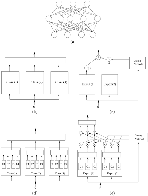
According to the levels of hierarchy involved, hierarchical networks can be divided structurally into the following categories (Figure 6.5).
One-level (i.e., structurally flat) networks. This is exemplified by the traditional MLP that has a "single-network" structure shown in Figure 6.5(a).
Two-level modular structures. By adopting the divide-and-conquer principle, the task is first divided into modules, and then the individual results are integrated into a final and collective decision. Two typical modular networks are (1) mixture-of-experts (MOE), which uses the expert-level modules (cf. Figure 6.5(c)); and (2) the decision-based neural networks (DBNN) based on the class-level modules (cf. Figure 6.5(b)). See Section 6.3 and Chapter 7 for details.
Three-level hierarchical structures. To this end, the divide-and-conquer principle needs to be applied twice: one time on the expert-level and another on the class-level. Depending on the order used, this could result in two kinds of hierarchical networks: one with an experts-in-class construct and another a classes-in-expert construct, as depicted in Figures 6.5(d) and 6.5(e). These two hierarchical structures are further discussed in Section 6.4.2.
Figure 6.5. Several possible hierarchies in NN structures: (a) Multi-layer perceptrons, (b) decision-based neural network, (c) MOE network, (d) experts-in-class network, and (e) classes-in-expert network.

6.4.1. Hierarchical Mixture-of-Experts
A popular hierarchical learning model is the hierarchical mixture-of-experts (HME) network [167]. Many theoretical derivations of HME, which is basically a Bayesian belief network, have been proposed (e.g., [161, 167, 389, 390]). Given a pattern, each expert network estimates the pattern's conditional posterior probability on local areas of the input space, and the gating network computes the conditional probability, which represents the likelihood of the expert subnet producing the correct answer. The final output is the weighted sum of the estimated probabilities from all the expert networks.
Figure 6.6 illustrates the architecture of a K-output HME classifier. The experts and gating networks in the HME can take any form as long as the information about the probability-generating function for each expert is known. In most cases, the HME classifier adopts the generalized linear models (GLIM) [167, 373] for the expert and gating networks. The GLIM model is described next.
To perform multiway classification over K classes, Jordan and Jacobs [167] and Waterhouse and Robinson [373] proposed that each expert network either adopts K-independent binomial models, each modeling only one class, or one multinomial model for all classes. For the former, the form of the binomial model in expert Ej is
Equation 6.4.1
![]()
where ![]() is the k-th element of the output vector
is the k-th element of the output vector ![]() , and
, and ![]() is the parameter vector associated with output node k. This is clearly reminiscent of the single-layer perceptron, with logistic output functions.
is the parameter vector associated with output node k. This is clearly reminiscent of the single-layer perceptron, with logistic output functions.
As for the multinomial model, the output of the lower-level expert Eij is
Equation 6.4.2

where ![]() is the k-th vector of the weight matrix Ψ(ij) corresponding to Expert Eij for class wi. This is equivalent to a single-layer perceptron with K outputs and a softmax output function. Richard and Lippmann [311] have shown that Eq. 6.4.2 can lead to the estimation of posterior probabilities. For simplicity's sake, the output of each expert network will henceforth be considered as the posterior probability estimated in a local area in the input space; that is, given an input vector x, the k-th output in expert network Eij is
is the k-th vector of the weight matrix Ψ(ij) corresponding to Expert Eij for class wi. This is equivalent to a single-layer perceptron with K outputs and a softmax output function. Richard and Lippmann [311] have shown that Eq. 6.4.2 can lead to the estimation of posterior probabilities. For simplicity's sake, the output of each expert network will henceforth be considered as the posterior probability estimated in a local area in the input space; that is, given an input vector x, the k-th output in expert network Eij is
Equation 6.4.3
![]()
The HME also uses an auxiliary network known as the gating network, which partitions the input space into regions corresponding to the various expert networks. The j-th output of gij of the lower-level gating network models the probability that Expert Eij produces the correct answer, given the input vector x—that is, gij(x) = P(Eij|x). Jordan and Jacobs [167] implement the gating network by the softmax function:
Equation 6.4.4

where ![]() is the j-th weight vector of the gating network corresponding to Expert Ei. By combining Eqs. 6.4.3 and 6.4.4, the k-th output of the Expert Ei in the HME network is the following:
is the j-th weight vector of the gating network corresponding to Expert Ei. By combining Eqs. 6.4.3 and 6.4.4, the k-th output of the Expert Ei in the HME network is the following:
Equation 6.4.5
![]()
Notice that both the expert outputs and network weights (gating outputs) are functions of input x.
The higher-level gating network in the HME combines the outputs of the lower-level experts as follows:
Equation 6.4.6
![]()
where ![]() is a K-dimensional output vector; and
is a K-dimensional output vector; and
Equation 6.4.7

where ![]() is the i-th weight vector of the higher-level gating network. For K-class classification problem, x is assigned to the k*-th class if
is the i-th weight vector of the higher-level gating network. For K-class classification problem, x is assigned to the k*-th class if
![]()
The training rules for the HME are based on the EM algorithm. The following details the procedures for estimating the parameters of the high-level expert. The extension to low-level experts is trivial. Suppose there are M experts and that each expert has K outputs. Define ![]() as the parameter set for the expert network Ej. Also define
as the parameter set for the expert network Ej. Also define ![]() as the parameter set for the gating network. The output vector of the whole HME network is defined as y = [y1, y2, ... , yk]T. If the input pattern x belongs to class wi, then yi = 1, yj = 0, and ∀j ≠ i. The likelihood function of the network output y is
as the parameter set for the gating network. The output vector of the whole HME network is defined as y = [y1, y2, ... , yk]T. If the input pattern x belongs to class wi, then yi = 1, yj = 0, and ∀j ≠ i. The likelihood function of the network output y is
Equation 6.4.8

where p(y|x, Ej) is the output likelihood function conditional on the expert network Ej. The p(y|x, Ej) is defined as follows:
Equation 6.4.9
![]()
Since only one yi is 1 (others are 0), the likelihood function of the output y is equal to the i-th posterior probability of the input x, that is,
Equation 6.4.10
![]()
The EM algorithm is used to maximize the following likelihood function:
Equation 6.4.11
![]()
Let W represents the set of parameters in the HME network (![]() ). Given the current estimate
). Given the current estimate ![]() , the EM procedure for maximizing Eq. 6.4.11 consists of two steps.
, the EM procedure for maximizing Eq. 6.4.11 consists of two steps.
1. | |
2. |
Chapter 3 provides a detailed discussion on the EM algorithm.
Notice that due to the nonlinearity of the softmax functions, it is impossible to obtain an analytical solution of ![]() and maxV
and maxV
![]() . Therefore, Jordan and Jacobs [167] use a gradient ascent method called the iteratively reweighted least-squares (IRLS) algorithm in the M-step optimization.
. Therefore, Jordan and Jacobs [167] use a gradient ascent method called the iteratively reweighted least-squares (IRLS) algorithm in the M-step optimization.
Unlike the Jordan and Jacobs proposal, where the exact values of yk are needed, this method requires only the class labels. Eq. 6.4.9 expresses the log-likelihood function conditional on the expert Ej as
Equation 6.4.15

By substituting Eq. 6.4.15 into Eq. 6.4.13, ![]() is rewritten as
is rewritten as
Equation 6.4.16

Since yi=1 if x(t) ∊ wi and yi = 0, if x(t) ∉ wi, Eq. 6.4.16 becomes
Equation 6.4.17

Then the derivatives of ![]() in Eq. 6.4.17 with respect to
in Eq. 6.4.17 with respect to ![]() are
are
Equation 6.4.18

where these relationships are used

![]()
and
![]()
The gradients for the gating network can be obtained in the same way. Eq. 6.4.18 shows that the gradient values are proportional to the estimation errors—(1 – Pwi|x(t), Ej)) in the first row or –P(wi|x(t), Ej) in the second row—and that the ratio of the contribution of this expert to the final estimation results in (hj (t)). Because the IRLS algorithm does not guarantee the updating process to converge to a global maximum, the learning algorithm used for the HME is actually not the EM, but the generalized EM (GEM) algorithm. Unlike the EM algorithm, in which convergence is guaranteed without setting learning parameters, some safeguard measures (e.g., appropriate choice of learning rate) are required for the IRLS algorithm to converge. Moreover, since the learning procedure for the HME has double training loops (at each M-step there are several iterations for IRLS), computation cost increases considerably.
6.4.2. Experts-in-Class and Classes-in-Expert Structures
An effective implementation of neural networks (NNs) hinges on (a combination of) locally distributed and hierarchical networks. Local and distributed processing is critical to fault tolerance and robustness in neural networks. A hierarchical design, on the other hand, often results in a more efficient network structure. Proper incorporation of expert-level modules and class-level modules into a hierarchical NN can improve computation and performance. A hierarchical NN comprises a variety of neural processing modules for which EM serves as a basic tool. In addition, the decision-based learning rule has proved to be effective in implementing a global (i.e., interclass) supervised training scheme. The structural designs and associated learning algorithms for decision-based neural networks are detailed in Chapter 7. There are many recent important applications involving fusion of information from completely different sources. The hierarchical NN structure can easily be extended to cope with multichannel information processing. Hierarchical neural networks with an embedded fusion agent offer an effective approach to channel fusion.
As mentioned in the previous sections, the MOE and HME adopt the expert-level partitioning strategies, whereas the DBNNs, GMMs, and EBFNs adopt the class-level partitioning strategies. A hierarchical NN configuration should allow the incorporation of both the expert-level and class-level modules. As discussed next, the selection of the inner blocks versus the outer blocks will lead to very distinctive hierarchical structures.
Experts-in-Class Hierarchical Structures
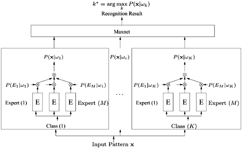
Figure 6.7 depicts the experts-in-class structure. The inner blocks comprise expert-level modules, while the outer blocks focus on the class level. A typical example of this type of network is the hierarchical DBNN [211], which describes the class discriminant function as a mixture of multiple probabilistic distributions; that is, the discriminant function of the class wc in the hierarchical DBNN is a class-conditional likelihood density p(x|wc):
Equation 6.4.19

Figure 6.7. Experts-in-class hierarchy for K-class classification problems. When applications have several experts or information sources, an experts-in-class hierarchical scheme can be applied; gating networks are omitted in the drawing. Like the baseline DBNN model, the minimal updating principle can be adopted to train the parameters in the network. P(Ej|wc) serves as the confidence indicator for the j-th expert in class c. It is a trainable parameter, and its value is fixed during retrieval time.

where p(x|wc, Ej) is the discriminant function of subnet c in expert j, and p(x|wc) is the combined discriminant function for class wc. The expert confidence P(Ej|wc) can be learned from the following EM algorithm. Define αj = P(Ej|wc) and set the initial value of αj = 1/M, ∀j = 1, …, M. The result at the m-th iteration is
Equation 6.4.20
![]()
Each expert processes only the local features from its corresponding class. The outputs from different experts are linearly combined. The weighting parameters, P(Ej|wc), represent the confidence of expert Ej producing the correct answer for the object class wc. Once they are trained in the learning phase, their values remain fixed during the retrieving (identification) phase. By definition, ![]() , where K is the number of experts in the subnet wc, so it has the property of a probability function. In conjunction with the expert-level (or rule-level) hierarchy, each hidden node within one class subnet can be used to model a certain local expert (or rule) with a varying degree of confidence, which reflects its ability to interpret a given input vector. The locally unsupervised and globally supervised scheme described in Section 7.4.2 can be adopted to train the expert networks (cf. Figure 7.8).
, where K is the number of experts in the subnet wc, so it has the property of a probability function. In conjunction with the expert-level (or rule-level) hierarchy, each hidden node within one class subnet can be used to model a certain local expert (or rule) with a varying degree of confidence, which reflects its ability to interpret a given input vector. The locally unsupervised and globally supervised scheme described in Section 7.4.2 can be adopted to train the expert networks (cf. Figure 7.8).
Classes-in-Expert Hierarchical Structures
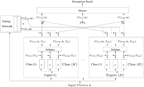
Figure 6.8 depicts the classes-in-expert structure. The inner blocks comprise class modules, and the outer blocks are the expert modules. Each expert has its own hierarchical DBNN classifier. The outputs of the hierarchical DBNNs are transformed to the posterior probabilities by softmax functions. In this scheme, the expert weighting P(Ej|x) is a function of input pattern x. Therefore, the importance of individual experts may vary with different input patterns observed.
Figure 6.8. Classes-in-expert hierarchy for K-class classification problems. In this scheme, the expert weighting parameters (P(Ej|x)) are functions of the input pattern x. The prior probability P(wi|Ej) could either be preassigned or estimated in a similar fashion as other prior probabilities such as P(Ej|wc) (cf. Eq. 6.4.20). This network can be viewed as a hybrid model of MOE and DBNN, where local expert networks serve as local classifiers. When applying such a hierarchical NN to channel fusion, each channel module can be regarded as a local expert with predetermined feature space.

This network adopts the posterior probabilities of electing a class given x (i.e., P(wc|x, Ej))—instead of the likelihood of observing x given a class (i.e., p(x|wc, Ej))—to model the discriminant function of each cluster. A new confidence P(Ej|x) is also assigned, which stands for the confidence on Expert Ej when the input pattern is x. Accordingly, the probability model is modified to become
Equation 6.4.21
![]()
where
Equation 6.4.22
![]()
with
Equation 6.4.23
![]()
The confidence P(Ej|x) can be obtained by the following equation:
Equation 6.4.24
![]()
Eq. 6.4.22 is one type of the softmax function. Its weighting parameter P(wc|Ej), just like P(Ej|wc) in Eq. 6.4.19, is made to satisfy the property of a probability function (i.e., ΣcP(wc|Ej) = 1). Consequently, P(wc|Ej) can be recursively estimated by the EM iterations in Eq. 6.4.20. The term P(Ej) can be interpreted as the confidence-level on Expert Ej, which can be learned by the EM iterations very similar to Eq. 6.4.20. The confidence level P(Ej) provides the key factor affecting the fusion weight P(Ej|x), which is the output of the softmax gating network. It can also be shown that P(Ej) can be learned by Eq. 6.4.20 with slight modification. Unlike the experts-in-class approach, the fusion weights need to be computed for each testing pattern during the retrieval phase.


