
3
Processing Crash Course
Now that the history lesson’s out of the way, let’s get things started with—what else?—tinkering with programming code. It’s time to dive into Processing and get those twitchy fingers going with something productive—creative coding. Don’t worry if you’re not a coding ninja. We’ll start with simple examples and work our way up to the harder stuff.
What’s Processing?
Have you ever had an idea you wanted to try out but didn’t have any idea where to start, how to create it, or what to do? We’ve all been there before. Maybe you were stumped because you didn’t know how to program or only understood the very basics. Perhaps you were simply short on cash and couldn’t scrape together enough under-the-couch-cushion treasure to buy a programming application such as Microsoft Visual Studio. Or maybe the problem was Mac or Linux hardware that was a little lacking in the options category.
Enter Processing. This open-source, cross-platform creative coding application is an ideal tool for those who want to create interactivity, drawings, and animation. Interested in drawing or generative art?
Processing does that. Have a game idea? Sketch it out on Processing. Want to track user movement on a webcam’s video stream? Processing, Processing, Processing!
Of course, Processing isn’t the only fish in the sea. There are other creative coding applications out there—openFrameworks, Cinder, Flash, and oodles of others—but Processing is a shining star for two reasons. First, it has an easy learning curve even for a beginner. The second reason it’s my first choice? A vast library of add-ons. Extra stuff and endless choices are nutritious brain food for tinkerers.
Getting Processing
It’s even easy to get. Fire up a browser, and navigate to the home of Processing—processing.org (Figure 3-1). Here you’ll find the most up-to-date information on Processing, view reference material, ask questions in the forum, and download the latest version of the application.

FIGURE 3-1 Download Processing at processing.org.
Click the link “Download Processing” or navigate to processing.org/download. Under Processing 2.0, you’ll have to choose your operating system (Figure 3-2), so you’d better know it. Windows users have the option of the 32- or 64-bit version, so get the one that matches your system. Also important? Remember where you download the application on your computer.
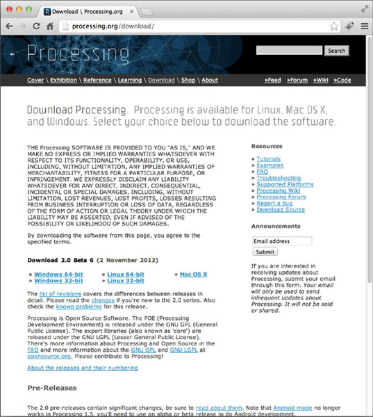
FIGURE 3-2 Make sure that you pick the correct version for your operating system. It’s 64-bit only for Mac users.
• Windows XP and Windows 7
• Mac OS X 10.6 and later versions
• Ubuntu Linux 9.04
For the purposes of this book, we’ll stick to the differences between Windows and Mac operating systems only. Of course, you Linux users are out there, but you’re always able to extrapolate the relevant content and figure it out. Isn’t that the secret handshake of the Linux club anyway?
Installing Processing on Mac OS X
Remember that Processing zip file you downloaded from processing.org? Now you need to find it. The default download location is the Downloads folder. Find the download, and double-click on it to unzip the contents. When you unzip on Mac OS X, the full file contents usually magically appear in the same location as the zipped file. Every now and then, you might be prompted for a different location. Usually that’s what happens when I’m focused on other things.
If you unzipped correctly (and you probably did), you should have the Processing application. Open a new Finder window, and drag the Processing.app file to your Applications directory.
After you successfully drop the Processing.app in the Applications folder, open the Applications folder. Find the Processing application, and launch it by double-clicking on it. Because you’re an “Apple person,” you can skip the next Windows bit.
Installing Processing on Windows
Remember a few minutes ago when you downloaded the Processing zip file from processing.org? You need to find it and then double-click on it to unzip the contents. Typically on Windows machines, the contents of zip files are unzipped right in the same location. You could, by chance, be prompted for a different location, so pay close attention to where you are and what you’re doing even when undertaking a task that is this mundane.
Drag the Processing folder to your C:Program Files (x86) if you’re using a 32-bit version of Windows. You 64-bit users, place the folder in C:Program Files. Once done, double-click on processing.exe from within the new folder to launch Processing.
Processing: Mac versus Windows
Wherever your hardware allegiances fall, you’ll be relieved to know that whether you’re a Mac, a Windows, or even a Linux user, the Processing interface is very similar. The toolbar is refreshingly simple and short on extra buttons. Actually, the differences in the Mac and Windows user interface (UI) are only marginal, as you can see in Figures 3-3 and 3-4.
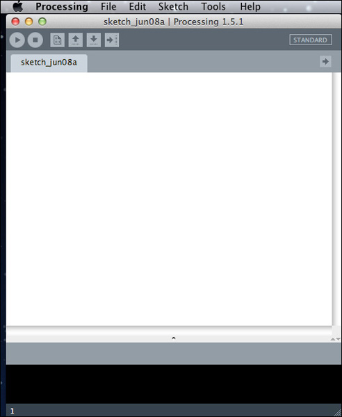
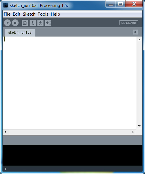
And that’s pretty much it. Wait, there’s one other thing you need to know. When you write code in Processing, it’s called a sketch. When Processing opens, it automatically creates a blank sketch.
There are several buttons in the top row of the interface. From left to right, there’s Run, Stop, New, Open, Save, and Export. Move your mouse over each icon, and you’ll be presented with the button’s name. These buttons do exactly what you think they do, but let’s look at each one quickly.
• Stop. Quits the sketch.
• New. Creates a blank sketch in a new window.
• Open. Launches an existing sketch in a new window.
• Save. Saves the current sketch.
• Export. Creates a standalone application for Windows, Mac, or Linux.
Honestly, Run and Stop are the only buttons you’re likely to use.
Hello, Circle!
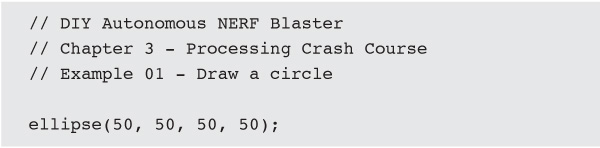
Most Programming 101 courses start with the same boring exercise: get your first application to display the phrase, “Hello, World!” We can all agree that this is lame. Well, here’s something else Processing does well—it delivers quick and easy output. Type the following into the code editor, and don’t forget the semicolon (every line of code needs to end with a semicolon):
![]()
You can probably see what’s going to happen just by looking at the code. Yes, we’re going to draw an ellipse—or for the layperson—a circle!
Here’s a look at how the numbers relate to the shape that’s created:
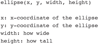
NOTE x, y coordinates refer to the center of the circle. All values are in pixels.
To see the circle, get your code input, and then click the Play button (Mac shortcut: COMMAND + R; Windows shortcut: CONTROL + R) to run the sketch. You should get something that looks like Figure 3-5.

You drew a circle! Pretty easy, huh? To draw a square, enter this, and hit Run instead:
![]()
Here the values are different from the ellipse, but the box is drawn in the exact same place. Rectangles don’t have a center origin point like an ellipse. A rectangle’s origin is the upper-left corner of the rectangle.
Go to the Menu, and choose File → Open. Navigate to the Examples folder you downloaded from autonerfblaster.com, find the Processing Crash Course folder, and choose the Example01 folder. Inside the folder, open Example01.pde. Here’s what you’ll see:
Let’s take a close look at this example and see what else is going on. If you have the example sketch open, you’ll notice the three lines of text at the top that describe the contents of the sketch. They should be grayed out a bit compared with the rest of the text.

Those three lines are called a comment. Comments are found in all forms of programming. They are simply plain English descriptions of what the pieces of code actually do. Comments are a great way to document code and help others to understand what you’re accomplishing through the code. They are also of great use when you are planning out your logic.
You can form comments in two ways using Processing. The first is like the preceding example: using a single-line comment mark, one much like this example:
![]()
The second way to form comments is using multiple lines of code. You could use this syntax to be a long-winded commenter:

Processing will ignore everything contained inside the slashes. This means that if you want to dump a detailed description in your sketch, you can. It’s also the perfect way to preserve chunks of code you’re too scared to delete. Simply comment them out, and they’re still there for reference or later use.
More Circles!
Let’s keep building on our ellipse example. One thing you may have noticed is that the display window Processing created was rather small. That happened because we didn’t tell Processing what size to make the window. Now let’s make it larger—because we can. On a line before the ellipse function, insert this snippet:
![]()
The size() function tells Processing to make the window 500 pixels wide by 500 pixels tall. At this point, you should have two lines of code. The first sets the window size, and the second draws the ellipse. Each line must end with a semicolon so that Processing knows that’s the end of the current instruction and to start looking for the next instruction. The following code is valid but is not encouraged:

We’ve got a black ellipse on a gray background, and it’s rather drab. Let’s add a little color. For the background, use the background() function, and supply a color value. To color an ellipse, use the fill() function, and provide the color value inside the parentheses, just like the background() function. To make a red ellipse, we can use the RGB value 255, 0, 0 or the hex value #ff0000. Mixing and matching color types is okay by Processing, too. For example, the background() function can contain a hex value, and the fill() function can have RGB values. Here’s the full code for a white background with a red ellipse:


Processing accepts the color values laid out in Table 3-1.
TABLE 3-1 Decoding Color Values
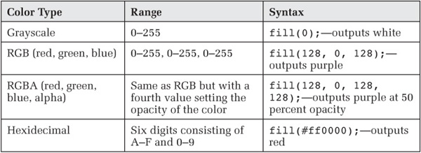
If you need help creating a color, try colorpicker.com.
Hit Play to see a red ellipse on a larger canvas. Feel free to change the colors and sizing of the ellipse now that you’re an old hat at creating circles using Processing.
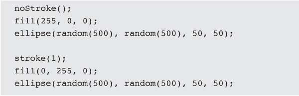
Let’s just keep on keepin’ on. Create a second and third ellipse by using the same ellipse instruction set as before, but make sure that you place them at different locations. Otherwise, you won’t see them. They’d be stacked on top of each other. To change each additional ellipse’s color, set the fill() function to a different value on each line prior to the ellipse() function, like this:

This code will yield ellipses of different colors and sizes. Hit Run and see.
What if you don’t care where the ellipse is placed on the sketch? This is exactly why we have the random() function. Simply enter the maximum value that you’d like, and Processing will grab a value somewhere between 0 and that number (Figures 3-6 through 3-8).
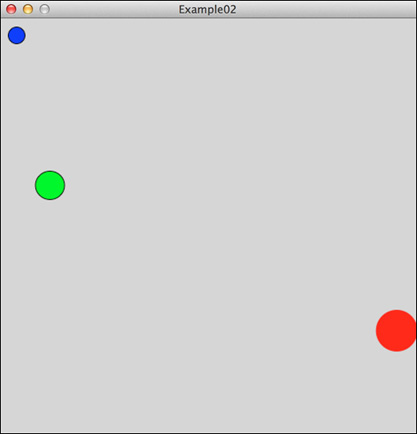
FIGURE 3-6 Note the red ellipse’s position. If you’re looking at these pictures in the book, it’s probably black and white, so make it happen on your screen so that you don’t have to take my word for it.


![]()
With this code, hitting Play generates a random position for that ellipse from 0–500 on the x and y axes. If you want to set a minimum and maximum value, you also could enter the minimum value first and then the maximum value. Using this method would always return a 50-pixel buffer on the outer edge of the display window.
![]()
Our last experiment deals with the black stroke that defines the edge of each ellipse. To get rid of that, simply use the noStroke() function.
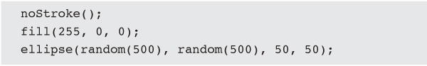
Now, only the fill color will be seen for each ellipse. If you want to add a stroke back to a subsequent ellipse, just use the stroke() function, and append a value in the parentheses of how thick to make the stroke in pixels.
Navigate back to the Examples folder, and open Example02. Your sketch should be very similar to this one. If not, you can use Example 2 to keep going as we jump into Example 3.
Save the Ellipses!
One thing all programmers want to do is make their lives easier. This is not being lazy; this is pure, unbridled efficiency. Let’s say that you need to place 100 circles on the screen. Would you want to do it by writing the ellipse() function 100 times? I hope not. That would be ridiculous. Fortunately, there’s a better way, and it’s called a for loop. A for loop is a fancy way of saying, “Do this x number of times.” For us, it’s a “draw a circle, at a random position, one hundred times” type of a loop.

Let’s analyze this bit by bit. In the parentheses we create an integer (int), define a variable name (i) for the integer, and then set it to zero. Next is the condition that needs to be determined. If this statement is true, the code in the brackets below the for line is executed. If the condition is false, the loop statement is terminated. The final i++ instruction is executed when the statement is true and adds 1 to the value of i. When it’s all said and done, the for loop will run 100 times.
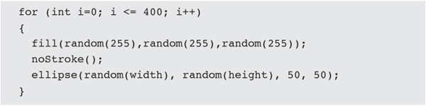
Now to inject our ellipse() function inside the brackets of the for loop to get it going. We’ll also make generous use of random() to give a completely different result every time our sketch is executed. Note that random() is used extensively for ellipse color and positioning. It also could be used for size, but for now let’s keep it tame.

Whoa, that’s not enough circles. Let’s increase the amount to 400. Let’s also say that our creation is going to be put online, but we don’t know the dimensions of where it will go. When we do find out, we do know that we will want to make the update as easy as possible. If it’s larger or smaller, we’ll have to go back and change the size and the ellipse() function. We can, however, do a quick edit to the ellipse line so that we don’t have to go back and change the value. We’ll use the reserved words width and height to make our lives easier. Width and height reference the window’s size, so whenever we change the size of the window, the ellipses will always stay within the new boundaries.
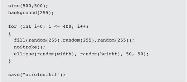
So now that all this effort has gone into creating this masterpiece, let’s save the output as an image. Once you’re done specifying the amount, color, and size of your circles, add the save() function to the end of your code, after the for() statement. In the parentheses, enter the filename for the image. There are four file formats available from which to select: TIF, PNG, JPG, and TGA. If a file extension is not specified, Processing will default to a TIF file.

The file generated will be saved in the sketch’s folder. The final code should be something like that in Figure 3-9.
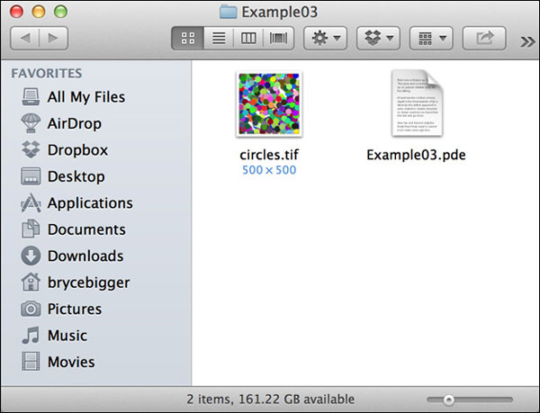
Open the Example 3 sketch to compare.
Let’s address the inevitable—you’re going to mess up. Processing will let you know when you do. Typically, it’s a typo or there’s no semicolon at the end-of-line of code. When you do mess up, Processing will try to point you to the location of the snafu and offer a suggestion as to the issue. (See the examples in Figures 3-10 and 3-11.) This makes it much easier to recognize the issue and fix it.


Don’t Skimp on Structure
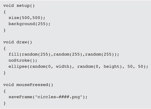
As your code gets more complex, it’s a good idea to break it up into easily digestible chunks. The first way to do this is to use the setup() and draw() functions. The setup() function holds all the initialization information for your sketch, such as size(), background(), and so on. Once everything in setup() has been executed, Processing moves on to the draw() function, aka meat of your code. Both these functions start with void because they don’t return any values. More advanced Processing code can send data from one function to another and return the crunched data back to the first function. For now, we’ll just stick to the basics.
To add an ellipse, one at a time instead of all at once, use these functions:

The draw() function executes as fast as possible, and in our sketch, it stops only when the sketch is closed. The effect animates like a colored-ball conga line on your screen.
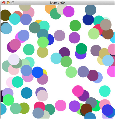
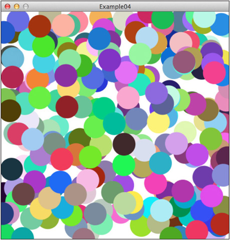
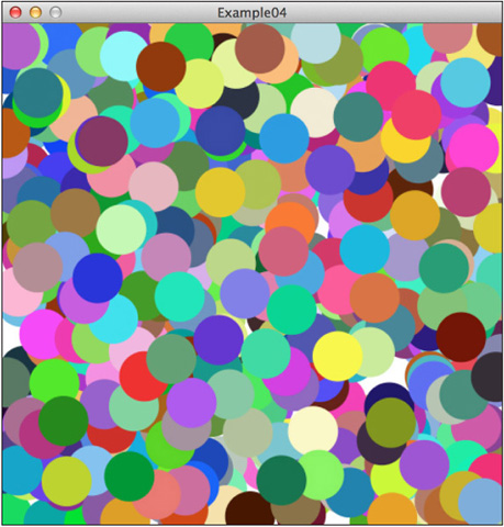
Now that we have structure, let’s talk about other options for interactivity. What, you may ask? How about performing an action every time the mouse is pressed? Let’s use a new function, mousePressed(), to trigger Processing to save the current state of the image or animation. We’ll use saveFrame() instead of save() so that multiple images can be saved instead of one image getting overwritten on every mouse press.

Including several number symbols (#’s) adds zeros to the padding of the filename, so images will be saved like circles-0001.png, circles-0124.png, or circles-9432.png to the sketch’s folder. Now you should have this as your code (Figures 3-12 through 3-14):
Let’s Draw
More interactivity starts with allowing the user to use the keyboard and mouse to provide user input. We’ll use the test conditions mousePressed and keyPressed to check whether the mouse or keyboard is being pressed. This is accomplished by using an if() statement, which takes a condition and decides whether or not to execute the code based on whether the condition is met.
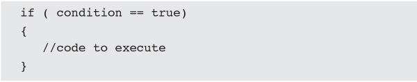
By default, an if() statement defaults to true, so it can be written like this as well:

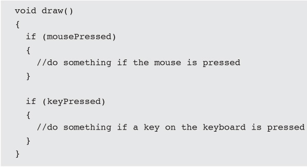
To test whether the mouse or any key on the keyboard is pressed, it would be written like this in our draw() function:
Now populate the code with some real data from our example.
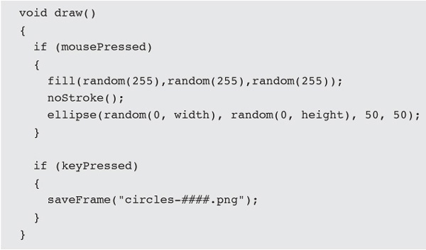
This code starts you out with a blank canvas. Every time the mouse is pressed, an ellipse is drawn randomly in the window. Any key pressed on the keyboard will save a new image.
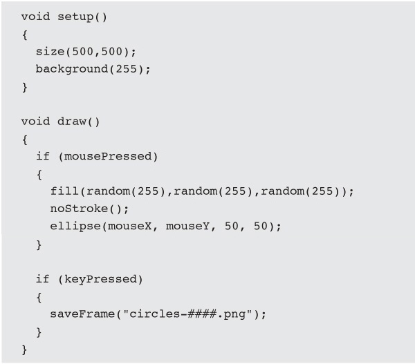
What would really make this great is if the ellipse were in the same location as where the mouse was pressed. Here’s how you do it—use mouseX and mouseY to get the coordinates of where you clicked the mouse.
![]()
Put it all together and you’ve got a drawing program that saves your art!
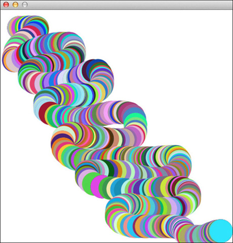
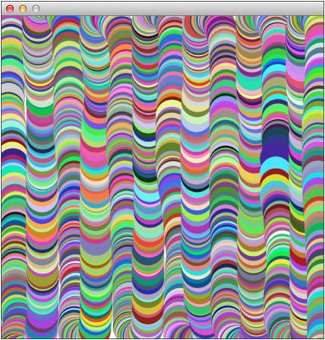
Now’s your chance to play around with your new skillset. Experiment with the color, shape, size, and opacity of the balls (Figures 3-15 through 3-17).

So that’s Processing. Quicker than you can say, “Hello world!” you have rad new software (Processing) and mad new skills (making circles), and these will come in handy when you build your automated NERF blaster. Next, we’ll tackle the microcontrolling minion of our autonomous NERF blaster—the Arduino circuit board.