
CHAPTER 6
Principles of Simulation Methods
This chapter provides an overview of simulation methods, their role in risk quantification and their relationship to sensitivity, scenario, optimisation and other techniques. We aim to introduce the basic principles in an intuitive and non-technical way, leaving the more technical aspects and implementation methods to later in the text.
6.1 Core Aspects of Simulation: A Descriptive Example
For the purpose of describing the fundamental principles of simulation methods, we shall consider a simple model in which:
- There are 10 inputs that are added together to form a total (the model's output).
- Each of the 10 inputs can take one of three possible values:
- A “base” value.
- A “low” value (e.g. 10% below the base).
- A “high” value (e.g. 10% above the base).
Of course, despite its simplicity, such a model (with small adaptations) has applications to many other situations, such as:
- Forecasting total revenues based on those of individual products or business units.
- Estimating the total cost of a project that is made up of various items (materials, labour, etc.).
- Forecasting the duration of a project whose completion requires several tasks to be conducted in sequence, so that the total duration is the sum of those of the individual tasks.
6.1.1 The Combinatorial Effects of Multiple Inputs and Distribution of Outputs
With some reflection, it is clear that there are 310 (or 59,049) possible combinations of input values: the first input can take any of three values, for each of which, the second can take any of three values, giving nine possible ways to combine the first two inputs. Once the third input is considered, there would be 27 possibilities, as each of the nine from the first two is combined with the values of the third, and so on. This sequence is shown in Figure 6.1 as the number of inputs increases.
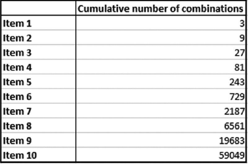
Figure 6.1 Number of Possible Combinations of Values for Various Numbers of Inputs, where Each Input can Take One of Three Values
The implicit assumption here is that the input values are independent of each other, so that one having a specific value (e.g. at, above or below its base) has no effect on the values that the others take; the consequence when there is dependence is discussed later. Additionally, we implicitly assume that each of the 10 base values is different to one another (in a way that each possible choice of input combination creates a unique value for the output), and is of a similar order of magnitude.
In general (and also as specifically assumed above), each input combination will result in a unique value for the output, so that the number of possible output values is the same as the number of input combinations, i.e. 310 or 59,049.
The question then arises as to how the output values are spread (distributed) across their possible range. For example, since each individual input varies equally (±10%) around its base, one might at first glance expect a more or less even spread. In fact, one can see that there are only a few ways to achieve the more extreme outcomes (i.e. where the output values are at the very high or low end of the possible range). For example:
- Only one combination of inputs results in the absolute lowest (or highest) possible value of the output, i.e. that combination in which each input takes its low (or high) value.
- There are only 10 ways for output values to be near to the absolute lowest (or highest) value, i.e. those combinations in which one input takes its base value, whilst all others take their low (or high) values.
There are many ways in which output values could be in the “central” part of the possible range (even if the precise values are slightly different to each other, and even though there is only one combination in which each input takes exactly its base value). For example, we can see that:
- There are 10 ways in which one input can take its high value, whilst all others take their base values. Similarly there are 10 ways in which one input takes its low value, whilst the others all take their base values. These 20 cases would result in output cases close to the central value, as only a single value deviates from its base.
- There are 90 ways in which one input takes its high value, one takes its low value and all remaining eight take their base values; these would result in output cases (very) close to the central value, due to the two deviating inputs acting in offsetting senses.
- There are many other fairly central combinations, such as two inputs taking high values, whilst two or three are low, and so on. Although the number of possibilities for such cases becomes harder to evaluate by mental arithmetic, it is nevertheless easy to calculate: it is given by the multinomial formula 10!/(L!H!B!), where L, H and B are the number of assumed low, high and base values (with L + H + B = 10), and ! is the factorial of the respective number (i.e. the product of all integers from one up to this number).
Figure 6.2 shows (calculated using this multinomial formula) the number of ways in which any number of inputs can take their low value whilst another number can take its high value (with the remaining inputs taking their base values). The highlighted areas indicate fairly central regions, in which the number of inputs that take their high value is the same as, or differs by at most one from, the number that take their low value. From this, one can see:
- The simpler cases discussed above (one, 10 and 90 combinations) are shown in the top left, top right and bottom left of the table.
- The more complex cases can be seen by close inspection: for example, there are 2520 possibilities in which three inputs take low values whilst two take high values, with (implicitly) the other five inputs at their base case, resulting in a fairly central case for the output.
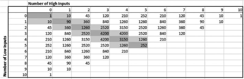
Figure 6.2 Number of Combinations Involving Inputs Taking a Particular Number of High or Low Values
When considered in percentage terms (of the total 59,049), we see in Figure 6.3 that:
- In 15.1% of cases, the number of high and low cases is the same (i.e. the sum of the diagonal of the table).
- In 28.4% of cases, the number of high and low cases differs by exactly one (i.e. the sum of the items immediately below and immediately above the diagonal).
- Thus, over 40% of cases are central ones in the sense that, with the exception of at most one input, the high and low values work to offset each other.
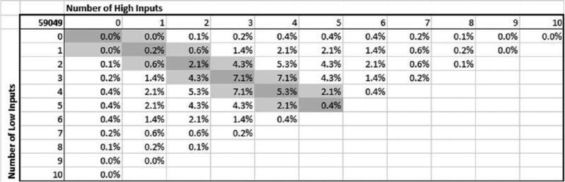
Figure 6.3 Percentages of Combinations Involving Inputs Taking a Particular Number of High or Low Values
In other words, the use of frequency distributions to describe the range and likelihood of possible output values is an inevitable result of the combinatorial effect arising due to the simultaneous variation of several inputs.
In a more general situation, some or all of the inputs may be able to take any value within a continuous range. The same thought process leads one to see that values within the central area would still be more frequent than those towards the ends of the range: for example, where the values for each input are equally likely within a continuous range (between a low and a high value), there are very few combinations in which the inputs are all toward their low values (or all toward their high ones), whereas there are many more ways in which some can be fairly low and others fairly high. Of course, due to the presence of continuous ranges in such a case, there would be infinitely many possible values (for each input, and in total).
6.1.2 Using Simulation to Sample Many Diverse Scenarios
The number of possible output values for a model is determined by the number of inputs and the number of possible values for each input. Generally speaking, in practice, not all possible output values can be explicitly calculated, either because their number is finite but large, or because it is infinite (such as when an input value can take any value within an infinite set of discrete values, or can be any value in a continuous range).
Simulation methods are essentially ways to calculate many possible combinations by automating several activities:
- The generation of input combinations.
- The recalculation of the model to reflect the new input values.
- The storage of results (i.e. of key model calculations or outputs) at each recalculation.
- The repetition of the above steps (typically, a large number of times).
For example, Figure 6.4 shows the simulated distribution of output values that results for the above 10-item model on the assumption that each input is drawn randomly from a range between zero and 100, in such a way that every input value would have equal likelihood.
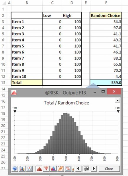
Figure 6.4 Simulated Distribution of Output Values for Uniform Continuous Inputs
A key aspect of simulation methods is that the generation of the input values is achieved by creating them using random sampling from a range (or distribution) of possible values. In other words, (Monte Carlo) simulation can be succinctly described as “the automated recalculation of a model as its inputs are simultaneously randomly sampled from probability distributions”. This contrasts with traditional sensitivity or scenario techniques, for which the input values used are explicitly predefined, and usually – by necessity – represent a small set of the possible combinations that may occur.
Note that the creation of randomness per se is not an objective of Monte Carlo simulation; rather, it is an implementation method to ensure that a representative set of scenarios is produced when the automated process is implemented.
Note the following about the output resulting from such repeated recalculations:
- The output is a finite set of data points (calculated by repeated recalculation of the model).
- The data points are a sample (subset) of the “true” distribution of the output, but are not a distribution function per se. Nevertheless, one often refers to a simulation as providing a “distribution of the output”; this is usually done for simplicity of presentation, but on occasion it can be important not to lose sight of the fact that the core output is a set of individual data points.
- The data set allows one to estimate properties of this true distribution, such as its average or the value in the worst 10% of cases, or to plot output graphically (such as a histogram of the frequency distribution of the points). It also allows one to calculate relationships between variables (especially correlation coefficients between inputs and an output), and to generate X–Y scatter plots of the values of variables (providing the relevant data are saved at each recalculation).
- The more recalculations one performs, the closer will be the estimated properties to those of the true distribution. The required number of recalculations needs to be sufficient to provide the necessary basis for decision support; in particular, it should ensure the validity and stability of any resulting decision. This will itself depend on the context, decision metrics used and accuracy requirements.
6.2 Simulation as a Risk Modelling Tool
Simulation and risk modelling are often thought of as equivalent, since in most business contexts the application of simulation methods is almost always to risk assessment; conversely, quantitative risk assessment often requires the use of simulation. However, there are some differences between the two: simulation is a method used to establish a large set of possible outcomes by automating the process of generating input combinations, using random sampling. There is no requirement per se that the underlying reason for the variation of an input is due to risk or uncertainty. Other reasons to use simulation include:
- Optimisation. The variation of input values could be a choice that is entirely controllable (rather than risky or uncertain), with the output data used as a basis to search for the input combination that gives the most desirable value. In general, however, simulation is often not a computationally efficient way to find optimal input combinations, especially in situations in which there are constraints to be respected. Nevertheless, simulation may be required in some cases.
- As a tool to conduct numerical integration. The first major use of simulation techniques was in the 1940s by scientists working on nuclear weapons projects at the Los Alamos National Laboratory in the USA: The value of the integral
 is equal to the average value of f(x) over the range 0 to 1. Hence, by calculating f(x) for a set of x-values (drawn randomly and uniformly) between 0 and 1, and taking their average, one can estimate the integral. The scientists considered that the method resembled gambling, and coined the term “Monte Carlo simulation”. This numerical integration method is simple to implement, and is especially powerful where the function f(x) can be readily evaluated for any value of x, but where the function is complex (or impossible) to integrate analytically.
In addition to these uses of simulation for non-risk purposes, there are also methods to perform risk quantification that do not use simulation, such as “analytic” methods and “closed-form” solutions; these are briefly discussed later in this chapter.
6.2.1 Distributions of Input Values and Their Role
From the above discussion, we see that probability distributions arise in two ways:
- Distributions of output values arise inevitably due to combinatorial effects, typically with more extreme cases being less frequent, as fewer input combinations can produce them.
- Distributions of inputs are used deliberately in order to automate the generation of a wide set of input combinations (rather than having to explicitly predefine each input combination or scenario). In such contexts, there is no requirement that the underlying reason that inputs vary is due to risk, uncertainty or general randomness:
- Where the purpose of the analysis is to assess all possible output values (as it may be in the above-mentioned cases of optimisation or numerical integration), it would generally be sufficient to assume that the possible values of any input are equally likely (i.e. are uniformly distributed). Only in special cases may it be necessary to use other profiles.
- Where the intention is explicitly for risk modelling, it is necessary (or preferable for accuracy purposes) to use input distributions that match the true nature of the underlying randomness (risk, variability or uncertain variation) in each process as closely as possible: it is clear that the use of different input distributions (in place of a uniform one) would affect the properties of the output distribution. For example, if an input distribution has highly likely central values, the frequency of more central values for the output will be increased.
On the other hand, in a risk modelling context, it is important to be aware of the (seemingly obvious) point that the use of a distribution is to represent the non-controllable aspect of the process, at least within the very particular context being modelled. This point is more subtle than it may appear at first: the context may be controllable, even where the process within that context is not. For example:
- When crossing a road, one can choose how many times to look, whether to put running shoes on, and so on; once a choice is made, the actual outcome (whether one arrives safely or not on the other side) is subject to non-controllable uncertainty.
- In the early phases of evaluating a potential construction project, the range for the cost of purchasing materials may be represented by a distribution of uncertainty. As more information becomes available (e.g. quotes are received or the project progresses), the range may narrow. Each stage represents a change of context, but at any particular stage, a distribution can be used to represent the uncertainty at that point.
Thus, an important aim is to find the optimal context in which to operate; one cannot simply use a distribution to capture that there is a wide possible range and abdicate responsibility to optimise the chosen context of operation! Indeed, one of the criticisms sometimes levelled at risk modelling activities is that they may interfere with the incentive systems. Indeed, if one misunderstands or incorrectly interprets the role of distributions, then the likelihood that such issues may arise is significant.
6.2.2 The Effect of Dependencies between Inputs
The use of probability distributions also facilitates the process of capturing possible dependencies between input processes. There are various types of possible relationship, which are discussed in detail later in the text. Here we simply note the main types:
- Those of a directional, or causal, nature (e.g. the occurrence of one event increasing the likelihood of another).
- Those that impact the way that samples from distributions are drawn jointly, but without directionality or causality between them. Correlation (or “correlated sampling”) is one key example, and copula relationships are another.
At this point, we simply note that any dependencies between the inputs would change the likelihood profile of the possible outcomes. For example (referring to the simple model used earlier), if a dependency relationship were such that a low value of the first input would mean that all other inputs took their low values (and similarly for the base and high values), then – since this one item fully determines the others – there would only be three possible outcomes in total (all low, all base or all high).
6.2.3 Key Questions Addressable using Risk-Based Simulation
The model outputs that one chooses to capture through a simulation will, of course, need to be the values of the key metrics (performance indicators), such as cost, profit, cash flow, financing needs, resource requirements, project schedule, and so on. In particular, specific statistical properties of such metrics will be of importance, such as:
- The centre of the range of possible outcomes:
- What is the average outcome?
- What is the most likely outcome?
- What value is the half-way point, i.e. where we are equally likely to do better or worse?
- The spread of the range of possible outcomes:
- What are the worst and best cases that are realistically possible?
- Is the risk equally balanced on each side of a central point?
- Is there a single measure that we can use to summarise the risk?
- The likelihood of a particular base or planned case being achieved:
- How likely is it that the planned case will be achieved (or not)?
- Should we proceed with the decision as it is, or should we iterate through a risk-mitigation and risk-response process to further modify and optimise the decision?
- Questions relating to the sources of risk, and the effect and benefits of risk mitigation, e.g.:
- Which sources of risk (or categories of risk) are the most significant?
- How would the risk profile be changed by the implementation of a risk-mitigation measure?
- What is the optimal strategy for risk mitigation?
6.2.4 Random Numbers and the Required Number of Recalculations or Iterations
Of course, all other things being equal, a more accurate result will be achieved if a simulation is run many times. Clearly, this also depends on the quality of the random number generation method. For example, since a computer is a finite instrument, it cannot contain every possible number, so that at some point any random number generation method would repeat itself (at least in theory); a poor method would have a short cycle, whereas superior methods would have very long cycles. Similarly, is it important that random numbers are generated in a way that this is representative and is not biased, so that (given enough samples) all combinations would be generated with their true frequency?
In general, for most reasonable random number algorithms, an “inverse square root law” is at work: on average, the error is halved as the number of recalculations (iterations) is quadrupled. An increase from 25 to 1600 recalculations corresponds to quadrupling the original figure three times (i.e. 1600 = 25.4.4.4); the result of this would be for the error to be halved three times over (i.e. to be about 1/8th of the original value). In this context, “error” refers to the difference between a statistic produced in the simulation and that of the true figure. However, such a true figure is rarely known – that is the main reason to use simulation in the first place! Nevertheless, on occasion, there are some situations where the true figure is known; these can be used to test the error embedded within the methods and speed of convergence. An example is given in Chapter 13, in the context of the calculation of π (3.14159…).
Although truly accurate results are only achievable with very large numbers of iterations (which at first sight may seem to be a major disadvantage of simulation methods), there are a number of points to bear in mind in this respect:
- Although many iterations (recalculations) may be required to improve the relative error significantly, the actual calculated values are usually quite close to the true figures, even for small numbers of iterations; in other words, the starting point for the application of an inverse-square-root law is one in which the error (or numerator) is generally quite low.
- The number of iterations required may ultimately depend on the model's objectives: estimating the mean or the values of other central figures usually requires far fewer iterations than estimating a P99 value, for example. Even figures such as a P90 are often reasonably accurate with small numbers of iterations.
- The error will (generally) never be zero, however many iterations are run.
- Usually it is the stability and validity of the decision that is the most important source of value-added, not the extremely precise calculation of a particular numerical figure. Thus, running “sufficient” iterations may be more important than trying to run many more (the use of a fixed seed for the random number algorithm in order to be able to repeat the simulation exactly is also a powerful technique in this respect, so that one can always work with the same [reasonably accurate] estimate).
- In business contexts, the models are not likely to be highly accurate, due to an imperfect understanding of the processes and the various estimates that are likely to be required. In addition, one is generally more interested in central values (in which we include the P90) than in unlikely cases.
- When one is building models, testing them, exploring hypotheses and drawing initial directional conclusions, the most effective working method can be to run relatively few iterations (typically several hundred or a few thousand). When final results are needed, the numbers of iterations can be increased (and perhaps the random number seed can be fixed, in order to allow repetition of the simulation).
- The reliance on graphical displays to communicate outputs (instead of on statistics) will generally require more iterations to be run; when it is intuitively clear that the underlying situation is a smooth, continuous process, participants will expect to see this reflected in graphical outputs. In particular, histograms for probability density curves that are created by counting the number of output data points in each of a set of predefined “bins” may not look smooth unless large numbers of samples are used (due to randomness, a point may be allocated to a neighbouring bin by a close margin). The use of cumulative curves and statistics can partially overcome this, but graphical displays in general will be apparently less stable than statistical measures.
6.3 Sensitivity and Scenario Analysis: Relationship to Simulation
Sensitivity and scenario techniques are no doubt familiar to most readers to a greater or lesser extent. We briefly describe these here for the purposes of comparison with simulation.
6.3.1 Sensitivity Analysis
Sensitivity analysis is the observation of the effects on particular model outputs as input values are varied. It can be used to answer many important (“What if?”) questions treated within a financial model, so long as the model has an input variable which corresponds to the desired sensitivity, and has a logical structure that is valid when the input value is changed.
The file Ch6.Time.Price.NoShift.xlsx (shown in Figure 6.5) contains an example of a simple business plan in which one has a forecast of cash flows over time, based on assumptions for margin, volume, capital expenditure and fixed cost. The net present value (NPV) of the first 10 years of these cash flows is $208.5m (shown in cell D13).
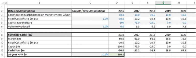
Figure 6.5 Generic Business Plan with Static Inputs
One could then ask what effect a reduction in the growth rate of the volume produced (cell C6) would have on the output (cell D13). Of course, this could be established by simply manually changing the value of the input cell (say from 5% to 2%). However, in order to see the effect of multiple changes in an input value, and in a way that is still live-linked into the model (i.e. would change if other assumptions were reset), Excel's DataTable feature is useful (under Data/What-If Analysis). Figure 6.6 shows an example of how to display NPV for several growth rate assumptions.
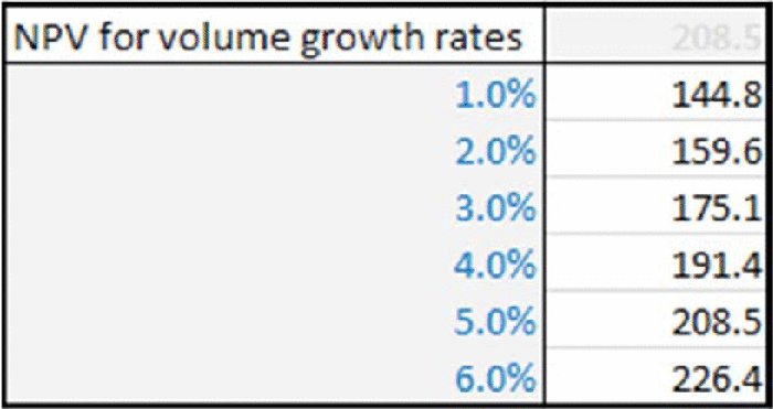
Figure 6.6 Sensitivity Analysis of NPV to Growth Rate in Volume
On the other hand, one can only run sensitivities for items for which the model has been designed. For example, if a model does not allow delaying the start date of the project, then a sensitivity analysis to such a situation cannot be performed. Therefore, the model may have to be modified to enable the start date to be altered; in an ideal world, one would have established (before building the model) the sensitivities required, and use this information to design the model in the right way from the beginning; the core principles of risk model design are discussed in detail in Chapter 7.
The file Ch6.Time.Price.Flex.xlsx (shown in Figure 6.7) contains formulae that allow for the start year of a project to be altered: these use a lookup function to map a profile of volume and capital expenditure from a generic time axis (i.e. years from launch) on to specific dates, which are then used in the model's calculations. One can see that the effect of a delay in the start date to 2017 is a reduction in NPV from $208.5m to $150.9m.
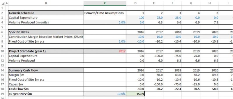
Figure 6.7 Business Plan with Flexible Start Date for Capital Expenditure and Production Volume
Similarly, Figure 6.8 shows a DataTable of NPV for various start dates.
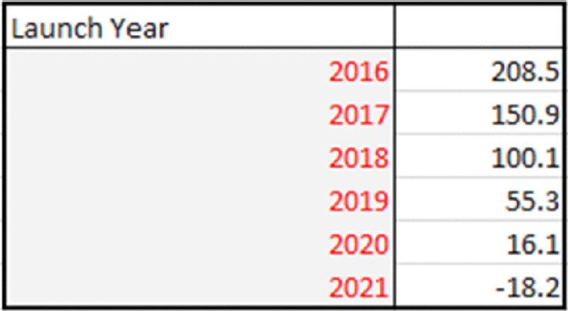
Figure 6.8 Sensitivity Analysis of NPV to Start Dates
One can also create DataTables in which two inputs are varied simultaneously. Figure 6.9 shows NPV as both initial volume and start dates are changed.
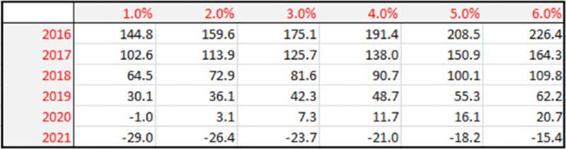
Figure 6.9 Sensitivity Analysis of NPV to Start Dates and Growth Rate in Volume
In relation to risk-based simulation methods, one can make the following observations:
- A core element of sensitivity and simulation modelling (and modelling more generally) is that models are designed so that they allow the relevant inputs to be changed; very often, inadequate attention is paid at the model design stage to the consideration of the sensitivity analysis that will be required, which needs to be done as it impacts the design of the (correct) model.
- For risk modelling, the inputs and model structure need to reflect the drivers of risk, and to capture the nature of that risk. For example, in a risk model it may be important for the project delay (after the planned launch in 2016) to be any figure, not just a whole number (such as if the delay were drawn randomly from a continuous range).
- Simulation modelling will change multiple inputs simultaneously (rather than a maximum of two when using a DataTable).
- In some cases (especially where other procedures are required to be run after any change in the value of an input), then – in place of a DataTable – it would generally be necessary to embed such procedures within a VBA macro that implements the sensitivity analysis by running through the various values to be tried.
These topics are addressed in detail in Chapter 7.
6.3.2 Scenario Analysis
Scenario analysis involves assessing the effect on the output of a model as several inputs (typically more than two) are changed at the same time, and in a way that is explicitly predefined. For example, there may be three scenarios, including a base case, a worst case and a best case. Each scenario captures a change in the value of several variables compared to their base values, and is defined with a logically consistent set of data. For example, when looking at profit scenarios, a worst case could include one where prices achieved are low, volumes sold are low and input costs are high.
Scenario analysis is a powerful planning tool with many applications, including:
- When it is considered that there are distinct cases possible for the value of a particular variable, rather than a continuous range.
- To begin to explore the effect on the model's calculations where several input variables change simultaneously. This can be used either as a first step towards a full simulation, or as an optimisation method that looks for the best scenario. In particular, it can be useful to generate a better understanding of a complex situation: by first thinking of specific scenarios, and the interactions and consequences that would apply for each, one can gradually consolidate ideas and create a more comprehensive understanding.
- As a proxy tool to capture dependencies between variables, especially where a relationship is known to exist, but where expressing it through explicit formulae is not possible or too complex. For example:
- In the context of the relationship between the volume sold and the price charged for a product, it may be difficult to create a valid formula for the volume that would apply for any assumed price. However, it may be possible to estimate (through judgement, expert estimates or market research) what the volume would be at some specific price points. In other words, although it may not be possible to capture the whole demand curve in a parameterised fashion, individual price–volume combinations can be treated as discrete scenarios, so that the dependency is captured implicitly when one changes scenario.
- The relationship between the numbers of sales people and the productivity of each, or that of employee morale with productivity.
- In macro-economic forecasting, one may wish to make assumptions for the values taken by a number of variables (perhaps as measured from cases that arose in historic data), but without having to define explicit parameterised relationships between them, which may be hard to do in a defensible manner.
Scenarios are generally best implemented in Excel by combining the use of lookup functions (e.g. CHOOSE or INDEX) with a DataTable: each scenario is characterised by an integer, which is used to drive a lookup function that returns the model input values that apply for the scenario. The DataTable is then used to conduct a sensitivity analysis as the scenario number is changed. (As for sensitivity analysis, and as also discussed in Chapter 7, where a model requires some procedure to be run after any change in a model input, then the scenario analysis would need to be implemented with a macro in place of the DataTable.)
The file Ch6.Time.Price.Scen.xlsx has been adapted to allow five scenarios of three input assumptions to be run (volume growth, start date and discount rates), with the original input values overwritten by a lookup function that picks out the values that apply in each scenario (the scenario number that drives the lookup function is in cell B2). Figure 6.10 shows the main model, and Figure 6.11 shows a DataTable of NPV for each scenario.
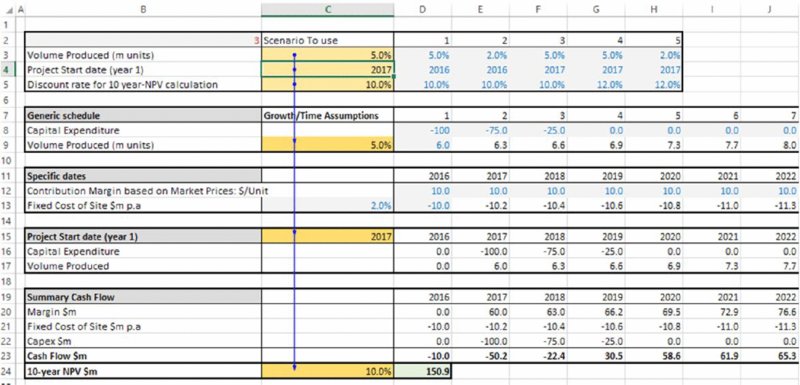
Figure 6.10 Business Plan Model Adapted to Include Input Scenarios
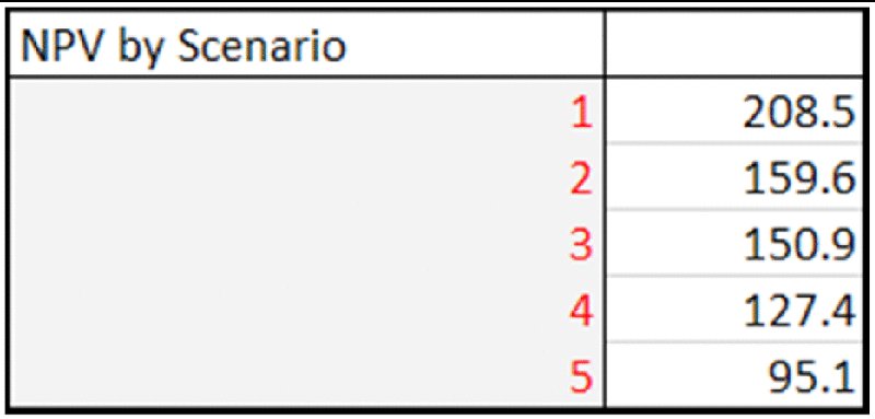
Figure 6.11 Sensitivity Analysis of NPV to Scenario
Limitations of traditional sensitivity and scenario approaches include:
- They show only a small set of explicitly predefined cases.
- They do not show a representative set of cases. For example, a base case that consists of most likely values will, in fact, typically not show the most likely value of the output (see earlier in the text).
- They do not explicitly drive a thought process that explores true risk drivers and risk mitigation actions (unlike a full risk assessment), and hence may not be based on genuine risk scenarios that one may be exposed to. Nor do they distinguish between variables that are risky or uncertain from those that are to be optimised (chosen optimally).
- There is also no explicit attempt to calculate the likelihood associated with output values, nor the full range of possible values. To do so would require multiple inputs being varied simultaneously and probabilities being attached to these variations. Thus, the decision-making basis is potentially inadequate:
- The average outcome is not known.
- The likelihood of any outcome is not known, such as that of a base plan being achieved.
- It is not easy to reflect risk tolerances (nor contingency requirements) adequately in the decision, or to set appropriate targets or appropriate objectives.
- It is not easy to compare one project with another.
6.3.3 Simulation using DataTables
As an aside, basic “simulations” can be done using a DataTable to generate a set of values that would arise if a model containing RAND() functions were repeatedly recalculated. Since the recalculation does not require anything in the model to be changed (apart from the value of the RAND() functions, which is done in any case at every recalculation), one could create a one-way DataTable, whose output(s) is the model output(s) and the inputs to be varied is a list of integers, each corresponding to a recalculation indexation number (i.e. the number one for the first recalculation, the number two for the second, etc.). The column input cell that would then be varied to take these integer values would simply be a blank cell in the sheet (such as the empty top-left corner of the DataTable). This approach would avoid any need for VBA.
In practice, this would generally be unsatisfactory for several reasons:
- The results would change each time the model recalculated, so that there would not be a permanent store of results that could be used to calculate statistics, create graphs and reports, and so on. One would need to manually copy the values to a separate range for this purpose.
- It would be inconvenient when working with the main part of the model, as to recalculate it when any change is made would require a full “simulation”, which would slow down the general working process, compared to running a simulation only when it was needed.
- It particular, it would be bad modelling practice to run a sensitivity analysis to a blank cell (in case some content were put into that cell, for example).
- It would be inflexible if changes needed to be made to the number of recalculations required, or to where results were placed, and so on.
This approach is generally not to be considered seriously for many practical situations, as the VBA code to run a basic simulation is very simple (although one may add more sophisticated functionality if desired); see Chapter 12.
6.3.4 GoalSeek
The Excel GoalSeek procedure (under Data/What-If Analysis) searches (iteratively) to find the value of a single model input that would lead to the output having a particular value that the user specifies.
For example, one may ask what volume growth would be required (with all other assumptions at their base value), so that NPV was $220m. From Figure 6.6, one can see that the figure is between 5% and 6%; to answer this question precisely using sensitivity techniques would require many iterations and generally not be very efficient.
The file Ch6.Time.Price.GoalSeek.xlsx (shown in Figure 6.12) has been adapted by placing the desired value for NPV in a cell of the model and calculating the difference, so that the target value is zero; this approach is generally more transparent and flexible (for example, the target value is explicit and recorded within the sheet, and it also allows for easier automation using macros).
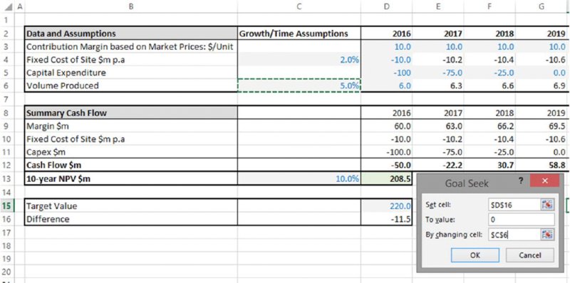
Figure 6.12 Finding the Required Growth Rate to Achieve a Target NPV
(Once the OK button is clicked in the procedure shown above, the value in cell C6 will iterate until a value of approximately 5.65% is found.)
Note that it is generally not a valid question to ask what combination of inputs (i.e. what scenario) will lead to a specific outcome; in general there would be many.
6.4 Optimisation Analysis and Modelling: Relationship to Simulation
This section discusses the relationship between simulation and optimisation analysis and modelling.
6.4.1 Uncertainty versus Choice
When conducting sensitivity and scenario analysis, it is not necessary to make a distinction between whether the input variable being tested is one whose value can be fully controlled or not. Where the value of an input variable can be fully controlled, then its value is a choice, so that the question arises as to which choice is best (from the point of view of the analyst or relevant decision-maker). Thus, in general, as indicated in Figure 6.13, there are two generic subcategories of sensitivity analysis:
- Risk or uncertainty context or focus, where the inputs are not controllable within any specific modelled context (and their possible values may be represented by distributions).
- Optimisation context or focus, where the input values are fully controllable within that context, and should be chosen optimally.
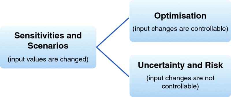
Figure 6.13 Relationship Between Sensitivities, Uncertainty and Optimisation
The distinction between whether one is faced with an uncertain situation or an optimisation one may depend on the perspective from which one is looking: one person's choice may be another's uncertainty and vice versa. For example:
- It may be an individual's choice as to what time to plan to get up in the morning. On a particular day, one may plan to rise at a time that takes into account the possibility that heavy rain may create travel disruptions, or that other unforeseen events may happen. These reflections may result in a precise (optimal) time that one chooses to rise. However, from the perspective of someone else who has insufficient information about the details of the other person's objectives for the day, travel processes and risk tolerances, the time at which the other person rises may be considered to be uncertain.
- It is a company's choice where to build a factory, with each possible location having a set of risks associated with it, as well as other structural differences between them. Once the analysis is complete, the location will be chosen by the company's management according to their criteria. However, an outsider lacks sufficient information about the management decision criteria and processes, and may regard the selection of the location as a process with an uncertain outcome.
- In some situations a company may be a price-taker (accepting the prevailing market prices), and hence exposed to the potential future uncertainty of prices (the same would apply if one's product sold at a premium or discount to such market prices). In other contexts, the company may be a price-maker (where it decides the price level to sell at); a modest increase in price may lead to sales increasing (if volume stays more or less constant), whereas a very high price would likely cause a catastrophic fall in sales volume, which leads to reduced sales in total. In such contexts, there would be an optimal price point.
The file Ch6.TimeFlex.Risk.Opt.xlsx (shown in Figure 6.14) contains an example portfolio of 10 projects, with the cash flow profile of each shown on a generic time axis (i.e. an investment followed by a positive cash flow from the date that each project is launched). Underneath the grid of generic profiles, another grid shows the effect when each project is given a specific start date (which can be changed to be any year number). In the case shown, all projects launch in 2016, resulting in a total financing requirement of $2270 in 2016 (cell D25).
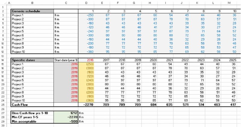
Figure 6.14 Project Portfolio with Mapping from Generic Time Axis to Specific Dates
However, the role of the various launch dates of the projects could depend on the situation:
- Risk or uncertainty context. Each project may be subject to some uncertainty on its timing, so that the future cash flow and financing profile would be uncertain. In this case, the modeller could replace the launch dates with values drawn from an appropriate distribution (one that samples future year numbers as integers), and a simulation could be run in order to establish the possible time profiles.
- Optimisation context. Where the choice of the set of dates is entirely within the discretion and control of the decision-maker. In this case, some sets of launch dates would be preferable to others. For example, one may wish to maximise the NPV of cash flow over the first 10 years, whilst not investing more than a specified amount in each individual year. Whereas launching of all projects simultaneously may exceed available funds, delaying some projects would reduce the investment requirement, but would also reduce NPV (due to the delay in the future cash flows). Thus, generically, a middle ground (optimal set of dates) may be sought, the precise values of which would depend on the objectives and specific constraints.
In this example (as shown in cell C29) the desired constraint may be one in which the minimum cash flow in any of the first five years should not fall below –$500m. Therefore, the case shown in Figure 6.14 would not be considered an acceptable set of launch dates.
The file Ch6.TimeFlex.Risk.Opt.Solver.xlsx (see Figure 6.15) contains an alternative set of launch dates, in which some projects start later than 2016. This is an acceptable set of dates, as the value in cell C28 is larger than that in C29. It is possible that this set of dates is the best one that could be achieved, but there may be an even better solution if one were to look further. (Note that in a continuous linear optimisation problem, an optimal solution would meet the constraints exactly, whereas in this case the input values are discrete integers.)
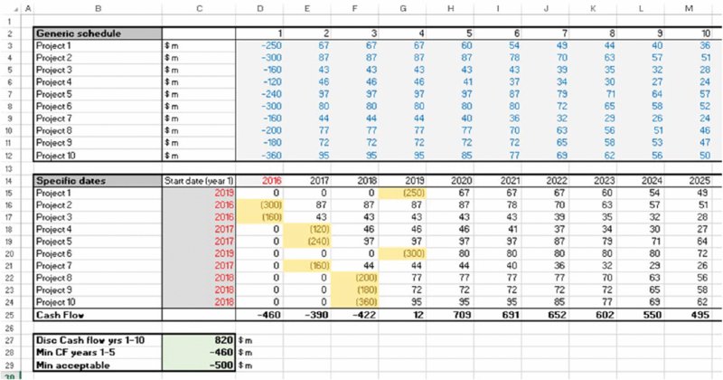
Figure 6.15 Delayed Launch Dates to Some Projects may Create an Acceptable or Optimal Solution
This example demonstrates the close relationship between simulation and core aspects of optimisation: in both cases, there is generally a combinatorial issue, i.e. there are many possible combinations of input and output values. Given this link, one may think that the appropriate techniques used to deal with each situation would be the same. For example, one may (try to) find optimal solutions by using simulation to calculate many (or all) possible model values as the inputs are varied simultaneously, and simply choose the best one; alternatively, one may try a number of predefined scenarios for the assumed start dates to see the effect of various combinations. In some cases, trial and error (applied with some common sense) may lead one to an acceptable (but perhaps not the truly optimal) solution.
Although such approaches may have their uses in some circumstances, they are not generally very efficient ways of solving optimisation problems. First, in some cases, properties implicit within the constraints can be used to reduce the number of possible input combinations that are worth considering. Second, by adapting the set of trial values based on the outcomes of previous trials, one may be able to search more quickly (i.e. by refining already established good or near-optimal solutions, rather than searching for completely new possibilities).
Therefore, in practice, tools and techniques specifically created for optimisation situations are usually more effective: Excel's Solver or Palisade's Evolver can be considered as possible tools. (The latter is part of the DecisionTools Suite, of which @RISK is also a key component.) For very large optimisation problems, one may need to use other tools or work outside the Excel platform (these are beyond the scope of this text).
Figure 6.16 shows the Solver dialog box that was used (Solver is a free component (add-in) to Excel that generally needs to be installed under Excel Options/Add-Ins, and will then appear on the Data tab; the dialog box is fairly self-explanatory).
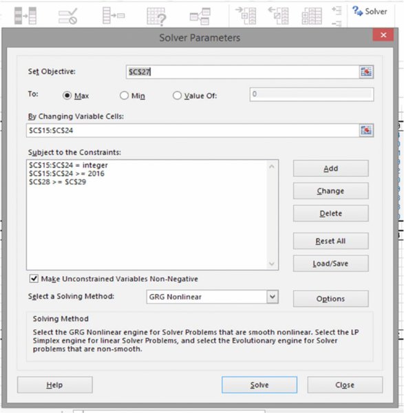
Figure 6.16 The Solver Dialog Box
It is important in practice to note that most optimisation tools allow for only one objective (e.g. maximise profits or minimise cost). Thus, qualitative definitions of objectives such as “maximising revenues whilst minimising cost” cannot typically be used as inputs into optimisation tools without further modification. Generally, all but one of the initial (multiple) objectives must be re-expressed as constraints, so that there is only one remaining objective and multiple constraints, such as “maximise profit whilst keeping costs below $10m and delivering the project within 3 years”.
Optimisation problems also arise when the number of possible options is low, but each option relates to a quite different situation. This can be thought of as “structural” optimisation, in which a decision must be taken whose consequence fundamentally changes the basic structure of the future, with the aim being to choose the best decision. For example:
- The choice as to whether to go on a luxury vacation or to buy a new car:
- If one goes on vacation and does not buy the car, one will thereafter have a very onerous journey to work each day (for example, a long walk to a bus stop on a narrow road, a bus journey to the train station, then a train journey, followed by another bus ride, and so on).
- If one buys the car, one will have a relatively easy drive to work in future, but not having had the benefits of the vacation one may become unhappy and quit the job!
- The choice as to whether a business should expand organically, through an acquisition or a joint venture, is a decision with only a few combinations (choices), but where each is of a fundamentally different (structural) nature.
- The choice as to whether to proceed or not with a project whose scope could be redefined (e.g. abandoned, expanded or modified) after some initial information has been gained in its early stages (such as the results of a test which provides an imperfect indicator of the likely future success of the project).
Figure 6.17 shows these two categories of optimisation situations.
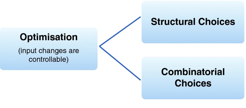
Figure 6.17 Categories of Optimisation Situations
Decision-tree methods are often used when faced with structural choices. In the following, we make some brief remarks about their benefits, beyond the purely visual aspect; however, a detailed treatment of them is beyond the scope of this text.
Figure 6.18 shows a simple example of a case in which the decisions to be taken are shown in a sequence: first, whether to go on vacation or buy a new car and second, the type of car that one buys in the case that the decision to buy a car is taken.
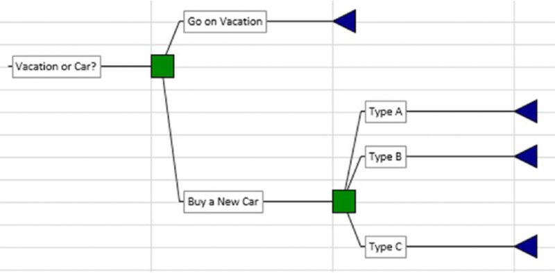
Figure 6.18 Simple Example of a Decision Structure
Note that when there are no further items appearing between the decisions that are in sequence (i.e. those concerned with the potential car purchase), then the tree shown in Figure 6.18 is the same as that shown in Figure 6.19 in terms of the ultimate available decisions, even though the sequencing is less visually explicit.
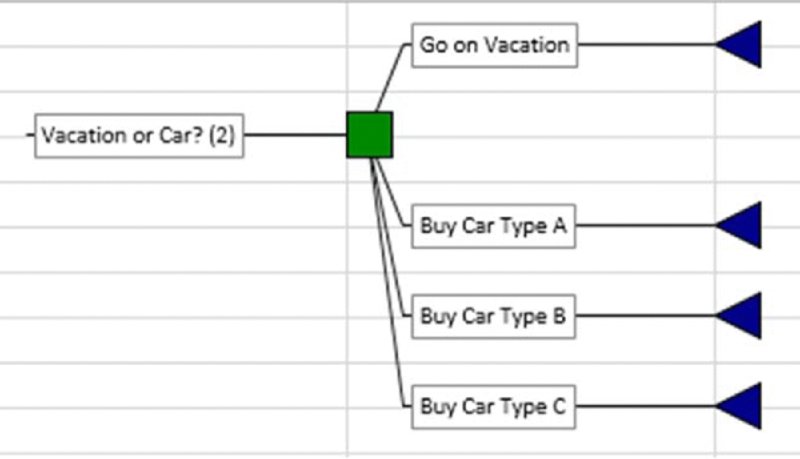
Figure 6.19 Sequential Decisions Presented as a Single Full Decision Set
Figures 6.18 and 6.19 were produced using Palisade's PrecisionTree software (which is part of the DecisionTools Suite). The quantitative (rather than the visual) benefit of such a tool is that it implements a backward calculation path that would be required if uncertainties occurred in between decisions within a decision sequence (by default, using the average outcome of each decision option). For example, whereas the tree shown in Figure 6.20 recommends that one stays in bed, the tree in Figure 6.21 recommends that one gets up. In each case, the average branch value (taking into account the probabilities shown by the branch percentages above the chance nodes, and the values shown below the branches) is calculated. However, whereas in Figure 6.20 this calculation can be done either from left to right or from right to left, in the structure of Figure 6.21 it can only be done from right to left (i.e. “backwards”).

Figure 6.20 Simple Example of Decision Tree with Future Uncertainty
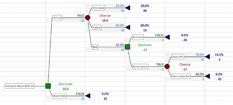
Figure 6.21 Decision Tree with Decisions Taken Following an Uncertain Outcome
The tree in Figure 6.21 shows a higher value than that in Figure 6.20; the difference (of 0.6) can be thought of as the “real options” value (value of flexibility) of having the choice (option) as to whether to go home or go to the cinema when one is having a bad day (as opposed to having no choices at all): to evaluate the basic decision as to whether to get up or not, one needs to know that this future potential possible behaviour has some value; hence the need for the backward process, which is not required in the pure “decision-making under uncertainty” context (as long as decisions are made using average future outcomes); Figure 6.20. Thus, there is a tight link between the topics of optimisation, real options and decision trees.
The backward calculation aspect within the software is perhaps its most important aspect, as the equivalent implementation in Excel can be quite cumbersome (and often overlooked as a required process), as shown in Figure 6.22.
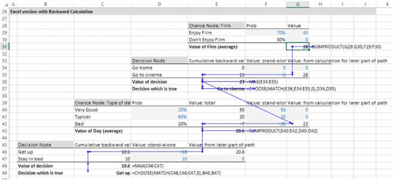
Figure 6.22 Excel Backward Calculation Path to Replicate Decision Tree Logic
6.4.2 Optimisation in the Presence of Risk and Uncertainty
Uncertainty may also be present in optimisation situations. Whereas the discussion associated with Figure 6.13 may seem to suggest that situations involving optimisation and those containing risk (or uncertainty) are mutually exclusive, there is, in fact, a more complex interaction between them: simply speaking, when a situation contains risk (or uncertainty), one is confronted with the question as to how to respond to that risk in an optimal way.
The optimal response to risk involves choosing optimally the context in which to act, which involves taking into account the risk or uncertainty within each context (as well as other decision factors). For example, it may be under our control as to whether we decide to make a journey by bus, bicycle or on foot. Each choice results in a base case (say average or expected) travel time that is different, and each has different costs. In addition, there is uncertainty within each option, which may affect the decision. Thus, it is possible that one may choose to walk on a particular day, in order to have a travel time that is more predictable than the other methods even if it may take longer on average.
An optimal risk mitigation (or response) strategy may have elements both of structural and combinatorial optimisation: structural optimisation about which context in which to operate, and combinatorial optimisation to find the best set of risk mitigation measures within that context.
Indeed, as discussed in Chapter 1, the essential role of risk assessment is to support the development and choice of the optimal context in which to operate (operating within the best structural context, mitigation and responding to risks within it), and to support the evaluation of a final decision taking into account the residual uncertainty and risk tolerances of the decision-maker.
6.4.3 Modelling Aspects of Optimisation Situations
As discussed above, optimisation and risk situations are inherently related, and many aspects of the underlying modelling issues are also similar. Nevertheless, there are some specific aspects that are worth summarising and emphasising at this point.
First, generally speaking, one needs to consider early on in the process what the correct tool and overall approach is, specifically whether tree, combinatorial, heuristic, mathematical or other approaches are the most suitable; this will also affect the basic platform (e.g. Excel or other) and tools (e.g. add-ins or other software) that should be used. Some optimisation situations can be challenging and complex: in particular, where the decision criteria are not based on future average outcomes but on other statistical measures, and where there is a sequence of decisions, then the optimal choice of decisions is harder; these stochastic optimisation situations are beyond the scope of this text.
Second, an explicit distinction between choice variables and uncertain ones needs to be made when using risk-based simulation or optimisation approaches (unlike when performing traditional sensitivity analysis, for example):
- In general, the inputs to Excel models are made up of numbers that are choice variables (to be optimised), uncertain variables (to be randomly sampled in a simulation) and other parameters that are fixed for the purposes of the model (e.g. scaling factors, etc.). In the general case, a single model may have items of each nature. For example, in the model shown in Figure 6.14, the generic cash flow profiles from the date of project launch could be uncertain, whilst the set of launch dates is to be optimised.
- Whereas in some specific application areas the uncertainty can be dealt with analytically, in general, simulation is required. This means that for every possible set of dates tried as a solution of the optimisation, a whole simulation would need to be run to see the uncertainty profile within that situation.
- Where a full simulation is required for each trial of a potential optimal solution, it is often worth considering whether the presence of the uncertainty would change the actual optimum solution in any significant way. The potential time involved in running many simulations can be significant, whereas it may not generate any different solutions. For example, in practice, the optimal route to travel across a large city may (in many cases) be the same irrespective of whether one considers the travel time for each individual potential segment of the journey to be uncertain or whether one considers it to be fixed. (There can be exceptions in situations where the uncertainty is highly non-symmetric, or due to the decision-maker's risk tolerances; in order to have more predictability of the total journey time, one may choose to walk one route rather than take the bus on a different route, even if walking is longer on average.)
- The RiskOptimizer tool (part of the Industrial version of @RISK), allows for a simulation to be run within each optimisation trial (which is powerful, but can be time consuming).
Third, from a process perspective, most optimisation algorithms allow for only one objective, whereas most business situations involve multiple objectives (and stakeholders with their own objectives). Thus, one typically needs to reformulate all but one of these objectives as constraints. Whilst in theory the optimal solution is found to be the same in each, in practice process participants would often be (or feel themselves to be) at an advantage if their own objective is the one taken as the single objective for the optimisation, and at a disadvantage if their objective is one that is translated into one of many constraints:
- Psychologically, an objective has positive overtones, whereas a constraint sounds more negative: an objective is something that one should strive to achieve; a constraint should be overcome.
- Whereas an objective is something that one is often reluctant to change, constraints are more likely to be de-emphasised, or to be regarded as items that can be modified or negotiated.
- When one's objective becomes expressed as only one item within a set of constraints, a focus on it is likely to be lost.
Fourth, models that are intended to be used for optimisation purposes sometimes have more demanding requirements on their internal logic than those that are to be used for simple “what-if” analysis. For example:
- Generically, the objective function of an optimisation model should follow a U-shaped (or inverted U-shaped) profile as the value of an input (choice) variable changes. The main exception is where the optimisation arises only as a result of constraints.
- A model that calculates sales revenues by multiplying price by volume may be sufficient for some simple purposes of sensitivity analysis, but if used to find the optimal price, then it would be meaningless unless volume is made to depend on price (with higher prices leading to lower volumes); otherwise an infinite price would be the best one to charge, which in practice would lead to sales being zero. As mentioned earlier, scenario approaches are often used if such dependencies are hard to accurately capture through parameterised relationships.
Finally, although optimisation situations often have a unique solution, there will often be many other possible sets of trial values that provide a close-to-optimal solution. This will be the case due to the U-shaped nature of the curve (which is flat at the optimal point, unless such a point is determined only by constraints). This feature of optimisation problems is part of the reason why heuristic or pragmatic methods can be so effective, as one may be able to find a very good solution with some trial and error and common sense. It can also explain why such techniques are hard to apply in practical organisational contexts; many similar variants of a close-to-optimal project will give a similar result, whereas some may be more favourable than others to specific process participants.
6.5 Analytic and Other Numerical Methods
This section provides an overview of analytic methods that are sometimes used in the context of financial and risk modelling activities. This provides some basis for comparison with simulation methods, and the applicability of each.
6.5.1 Analytic Methods and Closed-Form Solutions
In some cases, the distribution of a quantity (or of selected statistical properties of it) can be represented in an equation derived by mathematical manipulation of underlying assumptions (sometimes termed “analytic” techniques or “closed-form” solutions). Examples include:
- The Black–Scholes formula for the valuation of a European option (see below).
- The Huang–Litzenberger formulae for the calculation of the optimal composition of a financial portfolio, i.e. of the portfolio that has the minimum risk for any given expected return (also known as the Markowitz [efficient] frontier). The formula applies to the case where there is no constraint on the amount of each asset that may be held (such as no restrictions on short-selling or borrowing).
- In credit, insurance and reinsurance modelling, many analytic formulae exist in various areas, such as to calculate the distribution (or statistics thereof) of maxima (or extreme values) of random processes; this is the topic of extreme value theory (see Chapter 9 for more details).
An example of the first point above is the following: a European option is traded prior to an expiry date, and at expiration, the holder of a call option may buy an underlying asset, whereas the holder of a put option can sell it (each would be exercised at expiry if the asset price at expiry was above or below the exercise price respectively). The Black–Scholes formula gives the value of such options. It contains six variables: S (the current price of the underlying asset), E (the future exercise price at expiry of the option), τ (the time to expiry, or T – t where t is the current time and T the time of expiry), σ (the volatility of the return of the asset), r (the risk-free interest rate) and D (the constant dividend yield). The Black–Scholes formulae for call (C) and put (P) option values are:
where:
and N(x) is the cumulative probability to point x for the standard normal distribution.
Formulae also exist for the valuation of derivatives that are more complex than simple (vanilla) European options, and in some cases for where the underlying assumptions are generalised (e.g. where volatility may not be constant).
Closed-form (analytic) solutions are typically powerful to use when they are available. However, they also suffer from a number of potential drawbacks:
- Additional assumptions are generally required in order to be able to conduct the necessary mathematical manipulations to derive them. Thus, the “analytic” formulae are therefore still approximations to reality, so “model error” is nevertheless present (i.e. the conceptualised specification is not a perfect representation of reality). For example, in applications relating to financial options, derivatives and portfolios, it is often assumed that there are no transaction costs, or taxes, that certain processes are assumed to follow a normal (or lognormal) distribution and that some parameter values (such as volatility) are constant over time.
- The actual calculation of a specific result for a closed-form solution may be so complex that numerical approximations (such as simulation) are, in any case, required; as mentioned earlier, the origin of Monte Carlo methods was in the scientific arena, as a numerical tool to approximate the value of integrals.
- Even where possible to treat analytically, the models typically require a high degree of mathematical skill to understand and work with; as such they are often not practically applicable in business decision-making contexts, even where they may theoretically be so.
- In addition, in most practical applications relating to real-life business projects, closed-form solutions are generally not possible to derive:
- The processes that determine the inputs to a model, and the process by which inputs lead to outputs, are only partially understood and require judgement.
- There may be a lack of data to justify some assumptions with sufficient rigour.
- Even where the processes are understood and data are available, the mathematical manipulations are generally too complex. Even an apparently relatively simple set of calculations in an Excel spreadsheet (such as taking the maximum of two values, where each value itself results from other calculations that are derived from several inputs) would be difficult to evaluate in a closed-form sense, especially where the inputs may be themselves uncertain or have a distribution of possible values.
Where closed-form solutions are not appropriate or available, other numerical techniques sometimes exist for risk quantification, optimisation modelling and related areas. Examples include:
- Finite difference methods or finite element methods (part of the category of “grid-based” numerical techniques). These numerical approaches are widely used in scientific areas as well as in the financial area to solve partial differential equations. Binomial trees are another example of grid techniques.
- Linear, non-linear, dynamic programming and other optimisation techniques.
Once again, in practical business applications most of these techniques apply to specialised areas (e.g. optimisation of production schedules and product mixes), rather than being readily applicable to almost any situation.
The interested reader can find more details about these and further examples through simple internet or general literature searches.
6.5.2 Combining Simulation Methods with Exact Solutions
Simulation methods can sometimes be used in combination with exact solutions for specific purposes, including:
- Testing the accuracy of random number processes. For example (as discussed in detail in Chapter 13), one can establish an estimate of the value of π (3.14159…) using simulation. This could be used to test the accuracy of random number sampling methods, for example.
- Exploring the effect of uncertainty in values of the parameters used in exact analytic formulae (which typically assume that the parameter values are fixed). The volume of a cube is the product of its three dimensions, but what may the volume be if the measurement of each dimension is uncertain? This has applications to the modelling of uncertainty in oil reserves and mineral or resource volumes. Similarly, one may test the effect in the above options value formula of some of the parameters being uncertain (although often other mathematical approaches are also used to do that).
6.6 The Applicability of Simulation Methods
Simulation techniques have already found wide use in many applications. The reasons for this include:
- They can be used in almost any model, irrespective of the application or sector.
- They are conceptually quite straightforward, involving essentially the repeated recalculation to generate many representative scenarios.
- They are generally easy to implement, requiring only an understanding of fairly basic aspects of statistics and probability distributions, dependency relationships and (on occasion) some additional modelling techniques; the required level of mathematical knowledge is quite focused.
- They generally provide a surprisingly accurate estimate of the properties of the output distribution, even when only relatively few recalculations have been conducted (see earlier).
- They can be a useful complement to analytic or closed-form approaches; especially in more complex cases, simulation can be used to create intuition about the nature and the behaviour of the underlying processes and of the associated mathematics.
Thus, in many practical situations, simulation is the most appropriate tool, and indeed may be either the only, or by far the simplest, method available. Its use can often produce a high level of insight and value-added with fairly little effort or investment in time or money.