
CHAPTER 7
Core Principles of Risk Model Design
In this chapter, we highlight some core principles in the design of risk models. Many of these are similar to those in traditional static modelling, but there are, of course, some differences.
The extent of similarity is often overlooked, resulting in modellers who are competent in traditional static approaches being apprehensive to engage in potential risk modelling, or overwhelmed when initially trying to do so. Key similarities include:
- The importance of planning the model and its decision-support role, bearing in mind the context, overall objectives, organisational processes and management culture.
- The importance of keeping things as simple as possible, yet insightful, useful, but not simplistic.
- The importance of distinguishing the effect of controllable items (i.e. decisions) from that of non-controllable variables, both in terms of model building and in results presentation.
- The use of sensitivity thought processes as a model design tool.
- The need to build formulae that contain logic that is flexible enough to capture the nature of the sensitivity or uncertainty.
- The use of switches to control the running of different cases or scenarios.
- The need to capture general dependency relationships, both between inputs and calculations, and between calculated items.
- Very often, from the perspective of the formulae required in a model, it is often irrelevant whether the process to vary an input value is a manual one, or one that uses sensitivity techniques, or one that uses random sampling.
There are, of course, some differences between risk model design and that of traditional static models, including:
- The focus is on specific drivers of risk, rather than on general sensitivities.
- The structure and formulae in the model typically need adapting so that risks can be mapped into it. In particular, the impact of each risk must have a corresponding line item.
- The formulae may need to be more flexible or more general, for example to allow variations of values drawn from a continuous range, rather than from a finite set of discrete values.
- The model needs to be closely aligned with any general risk assessment process that is typically happening in parallel.
- The model needs to capture any dependencies between sources of risk, in addition to the general dependencies mentioned above; this topic is covered in detail in Chapter 11.
7.1 Model Planning and Communication
This section covers key aspects of the activities associated with the overall planning of a model and ensures that it is designed in a way that takes the likely communication issues into account.
7.1.1 Decision-Support Role
In any modelling context, it is clearly vital to remain focused on the overall objectives. In particular, the ultimate aim is usually to provide information to support a decision process in some way.
In a risk context, such decisions relate to:
- The implementation of actions to respond to risks and uncertainties.
- Decisions related to project design, structure and scope (these may not be traditional risks, but the potential to make a poor decision in respect of some particular issue is sometimes classified as a “decision risk”).
- The making of a final go/no-go decision on a project, based on the risk profile that results in the optimal context, i.e. where all other decisions have been considered, and the resulting risk profile is a residual.
A common shortfall in risk assessment activities in general is that so much attention is paid to the (less familiar) concepts of uncertainty and risk, that the necessary focus on the possible decision options is lost. This is generally due to the extra potential complexity involved in quantitative risk assessment activities, coupled with the fact that many participants are likely to have insufficient understanding of the real purpose and uses of the outputs.
7.1.2 Planning the Approach and Communicating the Output
A number of core points are vital about planning the overall approach to the modelling activities and to the presentation of results:
- Ensuring that a model is appropriately adapted to be able to reflect the key business issues. In particular, the ability to show the effect of decisions, not only uncertainties or risk, can be an important consideration (see later for an example).
- Adapting the model to reflect other likely communication needs. For example, when presenting results, one may desire to show items in categories, rather than as individual risks. If these items have not been considered in the model planning stage, significant rework of the model may be required later (often, this will be needed at the precise point in the project when there is no time to do so, i.e. shortly before results are presented).
- Planning communications around decision-makers' preferred media. Some decision-makers will prefer a more visual approach (such as graphs of distributions) and others may prefer more numerical approaches (such as key statistics). Similarly, some will wish to know the details of the methodology and assumptions, and others will be more interested in the overall message and recommendations.
- In general, there is a risk of excess information being shown, as the overall process is much richer than one based on static analysis: there is more information to be communicated about organisational processes and decision options, and there are more data and many more graphical possibilities.
- It is important not to overlook at what stage of the risk management process one is. For example, in the earlier stages, the focus may be on the effectiveness of risk-response measures or project-related decisions, and on the gaining of authorisation for them. In the later stages (once the effect of all sensible measures and decisions has been included), the focus may switch to a decision concerning the final project evaluation, i.e. whether to implement the project or not, given the revised economic structure and residual risks within the redesigned (optimised) project.
7.1.3 Using Switches to Control the Cases and Scenarios
Generally, one may need to use switches to control which set of assumptions is being used for the input values. There are many possible applications of this in risk modelling contexts:
- To be able to show the values of the base case static model (perhaps as the first scenario), as well as of additional static scenarios (if required).
- To show the effect of project-related decisions (“decision risks”).
- To show the effect of risk-related decisions, such as values that apply in a pre- and post-mitigation case.
Of course, the use of a switch is generally predicated on the model having the same structure for each scenario (or value) that the switch may take. The creation of a suitable common structure can often be achieved by making small modifications, in particular the use of items whose values are zero in the base case and non-zero in other cases. For example, line items could be added to represent the cost of various risk mitigation activities, and these included in the base model at a value of zero.
Note that there are various ways that switches may be used and implemented:
- A single (global) switch may change the values of all input variables.
- Multiple switches allow items to be activated or deactivated independently to others. In many cases, each decision may have its own switch, whereas switches for risk items would apply globally, at a category/group level or individually.
- One may wish to automate the process of ensuring that “risk” values are always used when a simulation is run, whereas base values are used once this is finished. This can be achieved by use of simple macros; an example is given later in the chapter.
- Where there are only two scenarios for each item (e.g. base case and risk case), one could use an IF function to implement the switch. More generally, there may be several scenarios, in which case another lookup function is usually preferable, especially the CHOOSE function.
An example of this latter point was provided in the discussion of scenarios in Chapter 6 (for example, see Figures 6.10 and 6.11).
The file Ch7.BaseSwitch.xlsx contains another simple example of a switch, shown in Figure 7.1. In this model, the percentage of sales volume that is lost to trade sanctions is considered to be zero in the base case, but is to be drawn from a uniform continuous distribution in the risk case (as discussed in more detail later in the text, the RAND() function will produce a uniform random number between zero and one, which is rescaled by the desired minimum and maximum, so that in this case, the result is a random value between zero and 10%).
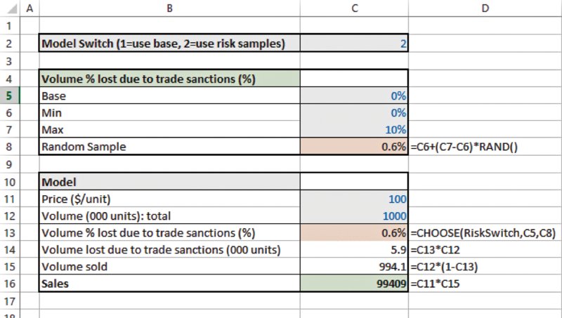
Figure 7.1 Use of Model Switch to Use Either a Base or a Risk Case Within the Model
7.1.4 Showing the Effect of Decisions versus Those of Uncertainties
The ability to distinguish the effect of decisions from those of uncertainties is a fundamental aspect of appropriate decision support.
Models can be used to show the effects of decisions by using multiple scenarios governed by model switches: for each decision, one defines “paired” scenarios that capture the effect of that decision being taken or not. In a static model, the values of the input variables would be altered as each decision scenario is run. In a risk model, the parameters of the input distributions may change as each decision is run.
One of the challenges in practice is to find the appropriate visual display for analysis, which involves both controllable decisions and uncertain factors:
- A focus on displaying the effect of decisions may help to support the appropriate selection of which decisions to implement (i.e. to find heuristically the optimal decision combination). Bespoke tornado diagrams (i.e. bar charts) may show the effect of each decision on some specific measure of the output (e.g. on the base, or on the simulated average or other measures), but they do not capture the uncertainty profile within each decision.
- Classical tornado diagrams (in simulation software such as @RISK) typically show the sensitivities in the output that are driven by the uncertainty of a variable within a specific decision context, but do not typically show the effect of decisions that may be taken. Thus, they are arguably mostly relevant in order to provide information about the key sources of uncertainty in a specific context (such as at the end of an assessment process to highlight the sources of risk that drive the residual, in principle non-controllable, uncertainty within the optimal context), rather than indicating which decisions are appropriate or have the most effect.
The file Ch7.DecisionsandRisks.Displays.xlsx contains an example of a bespoke “decision tornado” versus a “risk tornado”. Figure 7.2 shows a base model (contained in the worksheet BaseModel), which calculates the net present value (NPV) for a project. The worksheet BaseModelDecisions shows the input values that would apply for three possible decision scenarios for the project:
- The base project as currently planned.
- Moving the project to an alternative location (for example, closer to the end-user market), where it is estimated that volumes would be higher. However, there would also be higher fixed costs as well as an additional location charge (for example, local taxation) that would apply, and which is listed separately to the fixed costs.
- Remaining at the base location but using an alternative technology. The prices would be higher, and the variable cost percentage lower (i.e. a higher quality product with lower raw material waste), but the volumes would also be lower.
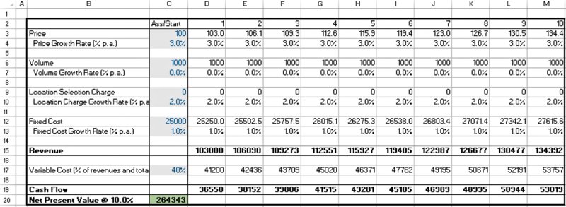
Figure 7.2 Calculation of NPV for a Simple Project
Figure 7.3 shows the specific input data for each scenario, as well as a DataTable that calculates NPV for each scenario (this uses the techniques discussed earlier, in which the scenario number drives a CHOOSE function).

Figure 7.3 NPV for Three Decision Options
The differences displayed in the bottom row of the table can be expressed in “tornado-like” form (a form of bar chart), as in Figure 7.4.
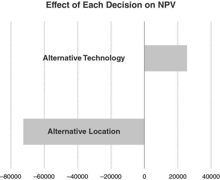
Figure 7.4 Tornado Chart for Decision Options
Assuming that one settles on the decision to use the alternative technology, one may conduct a risk assessment to establish key uncertainty drivers within this scenario. The worksheet RiskWithinScenario3 of the same file shows a simple case in which all inputs are assumed to vary in a ±10% range. The @RISK tool is used to run a simulation and to display a classical (correlation-coefficient) tornado chart, as shown in Figure 7.5.
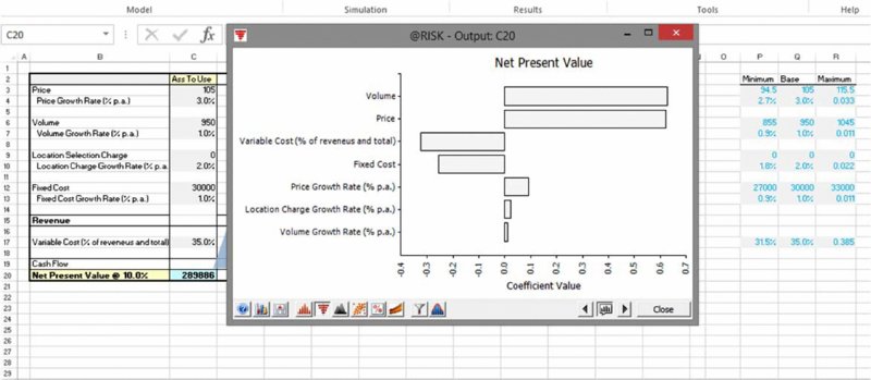
Figure 7.5 Tornado Chart for Uncertainties Within a Decision Option
Despite the importance of this issue, which was also partly addressed in the previous discussions concerning optimisation (Chapter 6) and risk prioritisation (Chapter 2), this distinction (between decisions and risks) is often overlooked in both static and risk contexts:
- Traditional sensitivity analysis or scenario analysis is often conducted without asking whether the items are controllable (choice or decision) variables.
- Models are very frequently built to show the effect of sensitivities, but not that of the available possible decisions. In particular, in group and organisational processes, the analysis of risks and uncertainties can dominate attention, resulting in a lack of sufficient explicit focus on the relevant decision possibilities.
- Even where the effect of some decisions is explicitly captured, very often the decisions that are available to be analysed within the model are not the full set of relevant decisions. For example, in some risk models, one may be able to compare the distribution of outcomes in the pre- and post-mitigation cases, but not to see the effect of other decisions that are not directly associated with risk (such as the effect of a decision to change the location at which a factory will be built, or the technical solution that will be employed).
Note also that the existence of any such decisions cannot be identified from a model, but only through processes that are exogenous (or separate) to the pure modelling activities.
In theory, there is a tight link between these issues and that of optimisation under uncertainty: in principle, if one could calculate the uncertainty profile of the outcome that would result for each combination of possible decisions, then the optimal combination could be chosen (by taking into account its overall effect and its uncertainty profile; it may increase average cost, whilst mitigating the worst possible outcomes, for example). In practice, a fully quantitative approach to such optimisation is often not possible or is excessively complex: one would need to have a model that captured the outcome and uncertainty profile for every decision combination, and that reflected the interactions between the decisions (for example, the effect of any particular decision may generally depend on which other decisions or mitigation options have been implemented). Thus, as discussed in Chapter 6, heuristic (pragmatic) methods are often sufficient to at least find close-to-optimal solutions.
7.1.5 Keeping It Simple, but not Simplistic: New Insights versus Modelling Errors
Whilst some spreadsheet models are built purely for calculation purposes, in many cases the modelling process has an important exploratory component. Whereas in later process stages there may be more emphasis on the calculated values, in earlier project stages the exploratory aspect can be especially important in generating insights around the project and its economic drivers.
Indeed, a model is implicitly a set of statements (hypotheses) about variables that affect an outcome, and of the relationships between them: the overlooking or underestimation of the exploratory component is one of the main inefficiencies in many modelling processes, which are often delegated to junior staff who are competent in “doing the numbers”, but who may not have the experience, or lack sufficient project exposure, or lack appropriate authority (or credibility) within the organisation, so that many possible insights are never generated or are lost.
The output of a model is a reflection of the assumptions and logic (which may or may not tell one anything useful about the situation); the modelling process is often inherently ambiguous (both in traditional static and in risk contexts):
- If one truly understood every facet of a situation completely, a model would be unnecessary.
- One must understand the situation reasonably well in order to be able to build a model that corresponds to it appropriately.
- To capture the reality of a situation, a model will need to have some level of complexity.
- Models can be made too complex, for example through the use of the wrong fundamental design, or being built in ways that use unnecessarily complex formulae, or by being too detailed, or simply by being presented in a confusing or non-transparent manner.
- Insight is usually generated when models have an appropriate balance between simplicity and complexity.
In this context, the following well-known quotes come to mind:
- “Every model is wrong, some are useful” (Box).
- “Perfection is the enemy of the good” (Voltaire).
- “Everything should be made as simple as possible, but no simpler” (Einstein).
Where a model produces results that are not readily explained intuitively, there are two generic cases:
- It is oversimplified, highly inaccurate or wrong in some major way. For example, key variables may have been left out, or dependencies not correctly captured, so that sensitivity analysis may produce ranges that are far too narrow (or too wide). Alternatively, the assumptions used for the values of key variables may be wrong, mistyped or poorly estimated. Of course, in such a situation, in the first instance one must correct any obvious mistakes.
- It is essentially correct in terms of the variables used, their relationships, data and input assumptions, but provides results that are not intuitive. In a sense, this is an ideal situation to face (especially in the earlier stages of a project); the subsequent process can be used to adapt, explore and generate new insights and intuition, so that ultimately both the intuition and the model's outputs are aligned. This can be a value-added process, particularly if it shows where one's initial intuition may be lagging, so that a better understanding is ultimately created.
In fact, there may be situations where useful models cannot be built:
- Where the objectives are not defined in a meaningful way. For example, doing one's best to “build a model of the moon” might not result in anything useful, at least without further clarification.
- Where basic structural elements or other key factors that drive the behaviour of the situation are not known or have not been decided upon. For example, it could prove to be a challenge to try to model the costs of building a new manufacturing facility in a new but unknown country, which will produce new products that still need to be defined and developed in accordance with regulations that have not yet been released, using technology that has not yet been specified.
- Where there are no data, no way to create expert estimates, or use judgements, and no proxy measures available. (Even in some such cases models that capture behaviours and interactions can be built, and used with generic numbers to structure the thought process and identify where more understanding, data or research is required.) In a risk modelling situation, with disciplined thinking, one can usually estimate reasonable risk ranges, although one needs to be conscious of potential biases, especially of anchoring and overconfidence (see Chapter 1).
In general, such barriers are only temporary and decrease as more information becomes available and project decisions are taken, and other objectives or structural elements are clarified. In principle, there is no real difference between static and risk models in this respect.
On the other hand, there can be differences between static and risk models in some areas:
- Risk models are often more detailed than static ones:
- There may be more line items required in order to capture the impacts of the risks (in some cases, such line items are used in aggregation calculations before the uncertainty is reflected in the model, such as when using the risk category approach discussed later).
- The input area will generally be larger. A single original input value that is subsequently treated as uncertain will have additional values associated with it, such as probability-of-occurrence and parameters for the impact range. In addition, there may be pre- and post-mitigation values of each of these parameters, as well as the cost of mitigation.
- The building of a useful risk model may only be able to happen at a slightly later stage than the building of an initial static model:
- Basic static models can be useful early in a process to “get a feel” about a particular project (for example, to support a hypothesis that a project may be unrealistic in its current form and should not be continued, or to help structure the process of identifying the nature of the further information and data requirements).
- The application of a full quantitative risk assessment at a very early process stage would generally not be an effective use of resources. Nevertheless, even basic qualitative statements of risk factors (perhaps with some selected basic quantification) can either reinforce the case for rejecting a project or help to define the flexibility requirements of any static model that is to be built to conduct further analysis.
- A well-structured risk model usually cannot be completed in its entirety before a general risk assessment process is complete, whereas a static model may typically be able to be completed earlier.
7.2 Sensitivity-Driven Thinking as a Model Design Tool
Since simulation is effectively the recalculation of a model many times, one core requirement is that any model is robust enough to allow the calculation of the many scenarios that are automatically generated through random sampling. In many respects, this requirement is the same as when one is conducting explicitly generated scenarios or traditional sensitivity analysis: the basic principle is that the logic and formulae in a model should be designed in a way that allows such sensitivities and scenarios to be run. These issues are discussed in more detail in this section.
Modelling can often be thought of as a process in which one starts with the objective or ultimate model output (such as profit), and asks what drives or determines this output (e.g. profit is equal to revenue minus cost), and building the corresponding calculations (i.e. with revenue and cost as inputs and profit as a calculated quantity). This process can be repeated (e.g. with the revenue determined as the sum of the revenues of each product group, each of which is itself the price multiplied by the volume for that product, and so on). Once completed, the model inputs are those items that are not calculated.
This “backward calculation” approach by itself is not sufficient to build an appropriate model. First, it is not clear at what point to stop, i.e. at what level of detail to work with. Second, there are typically many ways of breaking down an item into subcomponents. For example:
- Total sales could be broken down as:
- The sum of the sales for products (or product groups).
- The sum of the sales by customer (or by region).
- The number of products multiplied by the average sales figure for each.
- Etc.
- The cost of construction may be made up of:
- The cost of each type or category (e.g. materials, labour, energy), or that of more detailed categories (e.g. materials split into concrete, steel, wood, cabling, etc.).
- The cost by phase (e.g. planning, design and various build phases).
- The cost by component (e.g. office area, factory area, public areas).
- The cost by month of construction.
- As an aggregate base figure multiplied by cost escalation factors that change over time, and so on.
The use of “sensitivity analysis thinking” is a key technique to ensure that this backward calculation approach delivers an appropriate model: in practical terms, this means that when designing models, one should define as early as possible the specific sensitivity questions that will need to be addressed once the model has been completed. For model design purposes, such a thought process can be a qualitative one; there is no need to actually perform such sensitivities at this stage.
The definition of the sensitivities will result in many aspects of the model being defined as a consequence, and helping to ensure that:
- An appropriate choice is made for the variables used (i.e. the correct approach to break down items into possible subcomponents), and the necessary level of detail (i.e. where in the backward calculation process one should stop).
- Any required sensitivities can be run when the model is complete, and that drivers of variability that are common to several items are captured.
Note that if a (static) model has been built sufficiently robustly to allow any input to be varied, then (generally speaking):
- The nature of the process used to vary an input is not of significance: whether it is done manually, by an automated sensitivity tool (such as a DataTable) or by the random sampling of a distribution is essentially irrelevant (from the perspective of the formulae and calculations).
- Whether a change is made to a single input value or to multiple input values simultaneously will typically not affect the integrity of the model's calculations (there may be exceptional cases where this is not so). The sensitivity-thought process helps to retain the integrity of the calculations even as multiple input combinations are selected. Where “scenario thinking” is used to augment the core sensitivity thought processes, the model should be even more robust, as it should ensure that simultaneous variation of multiple input values is possible (as is required in simulation and combinatorial optimisation contexts).
The file Ch7.HRPlan.DataFixedSensRisk.xlsx provides a simple example that covers many of the issues above. Figure 7.6 shows a screen clip from the worksheet Data. This contains what is essentially a data set showing the expected number of people needed to be employed by a company for each year in a 5-year period. The only calculation is that of the total requirement over the 5-year period, which is 284 (cell H8).
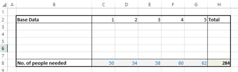
Figure 7.6 Simple Resource Plan
If one wished to explore the situation in more detail, one could then start to consider the factors that drive sensitivity of the number of people needed each year. One may conclude that this depends on the volume (i.e. on the work required), as well as on the productivity of the people. Thus, one may build a model as contained in the worksheet Orig, shown in Figure 7.7. In this model, additional assumptions are required for each of these driving factors. It may be the case that once best estimates of these factors are made, then the estimate of the number of people needed changes (as it is now a calculated quantity); in this case, the revised figure for the 5-year period is 275.
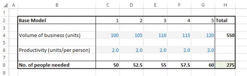
Figure 7.7 Resource Plan with First Approach to Calculations
Similarly, one may continue the process in which the volume of business depends on a periodic growth rate, and the productivity depends on productivity changes or improvements. Thus, as shown in Figure 7.8, and contained in the worksheet OrigSens, a revised model may show some changes to the values, as each of the volume and productivity figures (from year 2 onwards) is calculated from estimates of their driving factors; in this case, the new total is 268.
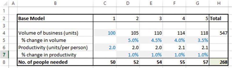
Figure 7.8 Resource Plan with Second Approach to Calculations
Of course, the process could continue if that were judged appropriate. On the other hand, one may decide that no further detail is required, but that a risk assessment of the base figure (268) could be appropriate.
As mentioned earlier, if a model is constructed to allow the running of the appropriate sensitivities (in this case, by varying the figure for the change in volume or productivity), then the process used to implement such variation is essentially of no significance from the perspective of the model's formulae and logic. The worksheet RiskView shows the implementation of this. Two switches have been created, one to show either base or risk values for the volume, and one to show those for the productivity (see Figure 7.9). Once again, for illustration purposes, the RAND() function has been used to create the ranges; this is not to suggest the appropriateness or not of the distribution in this context, rather to illustrate that the process used to vary an input is essentially irrelevant.
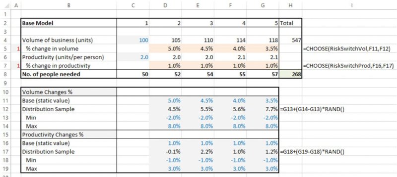
Figure 7.9 Resource Plan with Uncertainty Ranges
For completeness, Figure 7.10 shows the results of running a simulation, in terms of the distribution of the total number of people needed; the change from a “data set” to a traditional static model with sensitivity capability led to a modification of the estimated number of people required from 284 to 268, with the risk model showing that the required number would be less than 268 in approximately 80% of cases, and that a figure of 260 would be the average requirement.
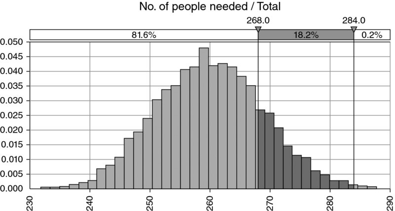
Figure 7.10 Distribution of Total Resource Requirements
7.2.1 Enhancing Sensitivity Processes for Risk Modelling
Although the importance of using sensitivity-driven thought processes represents a commonality in the design of static models and risk models, some additional considerations and modifications are usually necessary in risk modelling contexts.
In particular, whereas sensitivity (and scenario) processes focus on “What if?” questions, in risk assessment one also asks “Why?”, i.e. one aims to identify the factors that may cause variation in the item concerned (i.e. the “risk drivers”), whereas sensitivity analysis does not have this focus.
In practice, this would often lead to differences in the models that would be built.
First, the fact that one can conduct a sensitivity analysis in a traditional static model by changing the value of individual inputs does not mean that such changes actually reflect the true nature of the risk associated with that item; to do so may require that new line items are added or other modifications made to the model. Typical issues that arise in this respect include:
- A risk may affect only a portion of a line item. For example:
- A potential trade barrier (or import duties) may apply to only part of the volume, and this may also have an effect on part of the revenues and part of the cost, so that major modifications to many aspects of a model would be required if this risk were initially overlooked. Note that the model in Figure 7.1 provides an example of how each core component of a model may be structured in such a case. For the purposes of the discussion here (although the issue may appear trivial when reviewing the completed model in retrospect), if the starting point for the modelling process had been a model that simply calculated revenues by simply multiplying volume by price, then the later inclusion of the risk impact into the model would have required significant modification.
- Similarly, an exchange rate risk may affect only the export portion of the revenues, and a disruption to the supply of a specific raw material may partially affect production volume, or have an effect on highly specific parts of the cost structure, and so on.
- Risk assessment approaches are more likely to identify common drivers of variability that may be overlooked in pure sensitivity approaches. For example, one may be able to test the sensitivity of construction costs of a project by varying the daily rate for the cost of manual labour. However, the risk driver may be whether a new law concerning minimum wages would be passed by the government, in which case many other model items would be affected (not just the specific manual labour cost).
- The consideration of the drivers of the variability may guide the appropriate level of detail that the model should be built at, which may be different in the case that risk drivers are properly considered. For example:
- When dealing with a revenue forecast, the assessment of factors that could cause a variation in the price may include: whether a competitor enters the market, the nature of the promotional activity undertaken by the company, exchange rates, the overall macro-economic situation, and so on.
- The possible variation in production volume could be driven by: whether the overall product development project is delayed, whether the production facility breaks down, possible delays to material supplies or other problems with the supply chain, whether workers go on strike, whether there is a delay or failure in a process to have a patent awarded, whether to develop certain specialised technologies, and so on.
- The uncertainty in total labour cost may depend on the uncertainty in the number of labourers required, their cost per day and the number of days required. Once again, these would often not be required or done in a sensitivity-driven approach that only asks a “What if?” question about the effect of changes to the labour cost.
- A static model may not capture event risks (or may overlook them), particularly where their probability is less than 50% (so that the most likely case for each risk is that it would not occur). The use of risk techniques allows for event risks to be formally identified and included in a model in an unambiguous fashion (as discussed in Chapter 4).
Thus, the line items (or variables) within a risk model need to be defined at a level of granularity that allows the risks and their impacts to be captured. In other words, there is a “matching” between model items and the underlying identified risks (with each risk impact having a corresponding line item), and the impact of a risk will generally affect or interact with other model variables.
Second, a sensitivity-driven approach may not identify all of the key flexibilities required of a risk model, as in principle these relate directly to the identified risks and their nature. For example:
- In a sensitivity (“What if?”) approach, one may have built a model that allows for the on-stream date of a production facility to be delayed (for example, by whole periods within the Excel model, such as months, quarters or years). However, the nature of the delay uncertainty may be a continuous process, corresponding to partial model periods.
- A static model may include lookup functions that always return a valid value within the range of sensitivities that are run (for example, the effect of a 2-year delay to a project). However, the true nature of the possible delay may be something that can exceed the range of the lookup functions, and require structural adjustments or modifications to model formulae.
Thus, in a model designed using traditional sensitivity methods, from a mechanical perspective, one can often overwrite the inputs with random samples from distributions without causing numerical errors (although the continuous granularity of the time delay is an exception to this). However, the results produced by doing so are not likely to reflect the true nature of the risk or uncertainty in this situation: the inputs being varied may not correspond to the risks in the situation, the model may not have the right line items to reflect such risks and dependencies between risks and impacts may not have been appropriately reflected in the formulae (or variables) of the original static model.
7.2.2 Creating Dynamic Formulae
It is clear from the above discussion that a core modelling principle (for static and risk approaches) is to ensure that the logic and formulae within the model have the appropriate flexibility. However, it is frequently the case that this is not so. For example:
- Many models calculate tax charges using formulae that are valid only when taxable profit is positive, and do not account for cases where profit is negative (this may require capturing the accumulation and use of tax-loss carry-forwards, which would have an important cash flow effect compared to a direct tax rebate). Indeed, the consideration of the possibility of a tax loss may never arise when a static model is being built using sensitivity techniques, as the occurrence of a loss may arise only if multiple adverse events occur, and not through the occurrence of only one or two events, as would be detected in traditional sensitivity analysis.
- Some models use direct formula links, whereas indirect or lookup processes would allow for more flexibility. For example, when working out the value in local currency of an item expressed in a foreign currency, rather than creating a formula link between the item and a particular exchange rate, one could use the currency of each variable as a model input, with a lookup process used to find the relevant exchange rate; in this way, more items or currencies could easily be added to the model.
- Many models implicitly assume that the timing aspect of a project is fixed, for example that the production of a new manufacturing facility will begin on a specific date. In fact, there may be a risk relating to the on-time completion of the facility. In principle, there is no reason why such delays should not be considered as part of a sensitivity analysis in traditional modelling contexts. However, in many practical cases the “risk of a delay” is an item that often first appears only once a formal risk identification process has been conducted. At that point, a base model has often been completed, and there is insufficient time to adapt the model, because such a delay may affect many model items in different ways, so that many new formulae and linkages would need to be built, meaning that aligning the model with the actual risk assessment process would become challenging or impossible:
- Volume produced and sold may be fully shifted in time.
- The price level achieved per unit may not be shifted, as it may follow a separate time process related to market prices.
- Variable costs may be shifted in time.
- Some fixed overhead costs may remain even during the pre-start-up period, whereas others may be able to be delayed in line with the production volume.
The lack of sufficient flexibility in formulae arises most often in practice due to a combination of:
- A lack of consideration of the required sensitivities that decision-makers would like to see. (In a risk modelling context, this would also encompass cases where there has been a lack of consideration of the risks and their impacts.)
- A lack of consideration of how variations in multiple line items may interact.
- A lack of capability to implement the formulae required within Excel.
The creation of more flexible and advanced models revolves around removing hard-coded or structural assumptions and replacing them with values that can be altered as part of a sensitivity analysis (in which the original, structurally fixed case is one possible sensitivity or scenario); an example is given in the following.
7.2.3 Example: Time Shifting for Partial Periods
As an example of the difference between the formulae that are required in the case that a potential delay is discrete (as might suffice for sensitivity analysis) versus those that are required if potential delays are from a continuous range (as may be required for a risk model, especially if the delay is calculated as the result of other processes or is to be input as an expert estimate), we consider the following cases:
- Whole period delays.
- Partial period delays of less than one time grid within the Excel model.
- Partial period delays of any length.
Figure 6.14 (and the associated discussion and example file provided in Chapter 6) demonstrated the use of lookup functions to implement a capability to shift project start dates so that they are any year (expressed as a whole number). The reader can inspect the formulae used in the model, which are not discussed in more detail here; in the following, we present the more general case where the time shift could be any partial period.
The file Ch7.TimeShift.Various.xlsx contains an example in which an initial planned production volume can be delayed by various amounts, as shown in Figure 7.11. The formulae for both whole and short partial delays are relatively straightforward (two options are shown for the whole period delay, one using the INDEX function and the other using OFFSET). However, the formula that covers the case of any delay amount is more complex, and not shown fully in the screen clip due to its size; the reader can inspect the file. (As an aside, due to the complexity of this formula, and in particular the fact that it uses the same input cell in several places, it could be more robust and transparent to implement it as a VBA user-defined function; this is not done here for reasons of presentational transparency.)
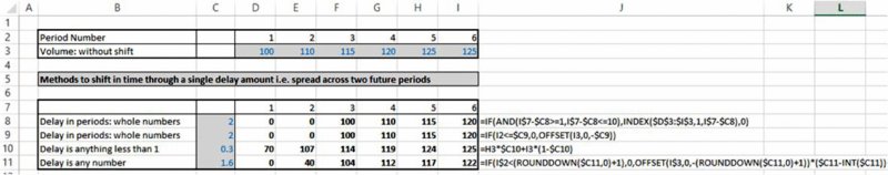
Figure 7.11 Various Approaches to Implementing Time Shifting in Excel
Of course, although the above example has the delay amount as an input, in many cases, it would be a calculated quantity that results from the impact of other risk factors. For example, a plan to launch a major new product that requires the construction of a production facility could be subject to delays such as those relating to:
- Building permissions required.
- An overrun of the construction project.
- Licences required for use of a particular technology.
- The development process for future products and technologies.
- Etc.
The file Ch7.ScheduleShift.xlsx contains an example in which there are three delay risks, each of which may happen with a given probability, and with an uncertain extent (in terms of monthly periods) that is described with minimum and maximum values. The aggregate delay is calculated as the maxima of the delay of each task (as the tasks are assumed to occur in parallel). This aggregate delay drives the updated production volume profile, using a calculation as shown in Figure 7.11. This structure is shown in Figure 7.12. One can also see that the model has been built with a switch, so that the base case (zero delay for each item) can also be shown.
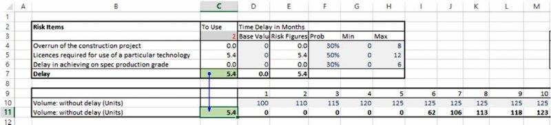
Figure 7.12 Calculations of Aggregate Delay As an Uncertain Amount
7.3 Risk Mapping and Process Alignment
Risk mapping involves describing the nature of the risks or uncertainties in a way that allows their inclusion within a quantitative model. As such, it is a core foundation of quantitative risk modelling. As mentioned in Chapter 2, it can be the most challenging part of the risk modelling process, as it requires an integration of many building blocks of risk quantification, such as:
- Ensuring that risks and impacts are precisely defined.
- Establishing the nature of risks and their impacts.
- Adapting the models to reflect the impacts of the risks, perhaps requiring additional line items, creating formulae that are dynamic and flexible (as discussed earlier in this chapter).
- Capturing dependencies between risks and between impacts (see later in this chapter and Chapter 11).
- Using distributions and data that are appropriate, with suitable approximations or estimates made where necessary (see Chapter 9).
- Aligning the risk modelling activities with the general risk assessment and decision process.
In this section, we highlight some key aspects concerning the nature of risks and their impacts, and the alignment with the general risk assessment process.
7.3.1 The Nature of Risks and Their Impacts
Clearly, a key aspect of being able to reflect the effect of a risk or uncertainty within a model is to establish its nature, including that of its impact.
Typical issues that one needs to consider include:
- Ensuring that the risk identification activities make an adequate distinction between business issues, controllable (decision) variables and risks or uncertainties.
- Ensuring that risks are described in a way that is appropriate for the approach taken. In particular, for risk aggregation and full risk models, one will need to find a way to express items in common terms (such as translating the effect of time delays into financial impacts, perhaps through volume or sales delays), and to avoid double-counting and overlaps of impacts.
- The core drivers or nature of the process: whether it is a risk event, a discrete process (such as having various possible distinct scenarios), a continuous process or a compound process (i.e. a mixture of discrete and continuous processes, such as a set of scenarios where a continuous range of values is possible within each scenario). It can also be helpful to consider whether the process is bounded or unbounded, as this may aid in the general understanding of the risk and in the selection of distributions.
- The time behaviour of the process (in a multi-period model), for example:
- Whether it can occur only once in total, or once during each period, or multiple times within each period.
- Whether there is a random fluctuation within each period around a long-term trend, or other aspects related to time-series modelling.
- Whether there is first a possible start time and a duration; if so, whether these also are uncertain.
- Whether the impact changes over time, such as fading.
- What is the nature of the impact? For example:
- Which model items are directly impacted (and which are only indirectly impacted through other calculations)?
- Are there interrelationships or overlaps between impacts of other risks?
- What other linkages are there with other risks and processes? For example:
- Are there common risk drivers or risk categories that should be reflected in the model?
- Do other general dependency relationships need to be captured as a result of the inclusion of the risk in a model, such as those between risk impacts or other core aspects?
- What dependency relationships exist between sources of risk, such as parameter dependencies or correlation? As discussed in Chapter 11, parameter dependencies require more intervention in a model than do sampling dependencies, which have less consequence for the formulae.
- What insights are provided by the above questions in terms of selecting the appropriate distributions to use for risks and/or their impacts (see Chapter 9 for a more detailed discussion)?
- What other relevant aspects need to be captured, so that the model is adaptable and its output is suitable for communication purposes? For example:
- Are categories required for communication purposes as well as risk purposes?
- How can the base case and the effect of decisions, as well as risk profiles, best be captured in the model?
7.3.2 Creating Alignment between Modelling and the General Risk Assessment Process
It is important to ensure that modelling activities are appropriately aligned with general risk assessment processes. This section covers the nature of such alignment activities; many of the points have been touched upon at various places in the text, so that the discussion here partly serves a consolidation purpose, and is therefore fairly brief, despite its importance.
Risk aggregation approaches require that risks and uncertainties are defined in a way that allows them to be expressed in common terms, and avoid overlaps or double-counting, both for any risk-occurrence events and for their impacts (as discussed in Chapter 3):
- This represents a modification in the information and data requirements compared to pure risk management approaches. Indeed, such topics may appear unnecessary or uninteresting to participants whose focus is on operational risk management.
- The capturing of the nature of the risks with sufficient detail and precision can be a challenge; even experienced risk management practitioners may not have had sufficient exposure to this specific area. The thought processes or concepts that are required in order to provide the appropriate information can be challenging to some participants. It can also be difficult to retain the attention of a group of participants, to explain additional concepts and to ensure that the appropriate deliverables result from group processes.
- An adequate distinction must be made between business issues, decision variables (controllable processes) and uncertainty variables, and the role of the general risk assessment (and modelling) process to treat these. For example, a “risk model” may, in fact, have a focus that is more of a decision-support nature, with the captured risks ultimately reflecting residual uncertainties.
Thus, there may be many aspects of the general risk assessment process that need adapting in order to be able to adequately build a full risk model:
- The modelling assumptions and inputs needed to design, build and use the results of models in fact (should) require a significant proactive role in specifying the nature of the required outputs from general risk assessment activities. It is important to reflect these directly in the process as far as possible, because if they are ignored, modelling analysts will ultimately need to make assumptions related to these points, even where such assumptions have not been debated within the wider project team. Thus, once initiated, an ongoing interaction between a general risk assessment process and the modelling activities linked to it is essential.
- There may be (real or perceived) differences in the requirements that participants in a general risk assessment process may have compared to the requirements of modelling analysts, and the alignment between their objectives will often ultimately need to be driven by top management.
It is important to gain agreement from senior management on the approach to be used to risk quantification, and ensuring that the consequences of this are communicated and implemented within the overall risk assessment activities. Clearly, the embedding of additional elements into the process can create a challenge, especially if expectations are not properly managed and communications are not sufficiently clear.
7.3.3 Results Interpretation within the Context of Process Stages
In practice, one usually passes through many stages of a process. The message and items to communicate may differ at each stage, or at least have a different focus:
- Core risk assessment and modelling stage. This is where the model is adapted to ensure that all relevant risks are captured, and their impacts and interdependencies reflected in the model. As discussed elsewhere, it will often also require that the more general risk assessment process is adapted to provide the correct inputs into a model. At this stage the focus will be on ensuring that:
- The model is free from errors.
- The risks are captured in a way that reflects their true nature and underlying properties (e.g. that risks that develop over time are captured appropriately and that no event risk is treated as being of an event or operational risk nature).
- The impact of each risk on the aggregate model's output makes sense and aligns with intuition (or alters that intuition and understanding of a situation).
- The risks can be presented in appropriate categories, and that base cases can be captured separately, and perhaps pre- and post-mitigation scenarios can be shown.
- The model will be adapted iteratively as the complete set of risks is identified and as the risk definition is made more precise, so that their impacts can be captured correctly in the model.
- Interim results presentation. Once a basic model is more or less complete, there could be a number of possible results and uses:
- It may immediately become clear that the project is too risky and should be cancelled.
- More generally, some risk-response measures and mitigation actions may be built into the project plans at little or no cost, whereas others may require specific escalation and authorisation (for the reasons discussed in Chapter 1, for example).
- This process stage may be iterative, as discussed earlier.
- Final results and decision stage. At this stage, the effect of all proposed and appropriate response and mitigation actions will have been included in the model and a final decision about a project's viability will need to be made, reflecting, for example, the average benefits as well as the exposure to potential adverse outcomes.
Note that as this process proceeds, one can generally state that:
- In the earlier stages, one may use a wide variety of measures and tools to analyse the model and its outputs, but one will typically not need to focus very precisely on the presentational aspects of individual activities. For example, one may look to a range of statistical measures, look at density and cumulative distributions, at ascending and descending forms, consider tornado graphs and scatter plots, experiment with the effect of different numbers of recalculations (iterations), and so on.
- In the later stages, or for senior management reporting, one may focus on a much more limited set of measures and wish to be able to present specific graph types in the way that management may desire. This may involve specific steps that may not be so relevant in the earlier stages (e.g. to be able to place and display risks within categories, or to be able to repeat a simulation exactly, or to show before/after-type analysis, and so on).
Questions about the output distribution are most relevant when the risk-response process (and the implementation of other project-related decisions) is complete. The resulting uncertainty profile is then one associated with residual risk in the optimal project structure, and is required for making a final decision that reflects the risk tolerances of the decision-maker (or of the organisation).
7.4 General Dependency Relationships
The capturing of dependencies between variables is one of the key foundations of modelling: Indeed, a model is, in essence, only a statement of such relationships, which one uses to perform calculations, test hypotheses or generate a better understanding of a situation; this contrasts with data sets (or databases), which contain lists of items but without relationships between them.
Of course, the nature and effect of any relationships within a model can be observed and tested with sensitivity analysis. Whereas the values shown in a model's base case may appear reasonable, if relationships are not captured correctly, then the model's calculations may either be fundamentally incorrect or will not reflect the true level of variation in the output when input values are altered. For example:
- Where the total cost of a project is estimated as the sum of several items, if such items in fact have a common driver, then a model that does not capture this would show sensitivities to the costs of individual items that are too low; in reality, a change in the cost of one item would be possible only if the cost of the others also changed, thus creating a wider range.
- Where the margin achieved by selling a product is calculated as the difference between the sales price and its input costs, then a model that does not reflect that both are closely related to the market price of an input raw material would show sensitivities to sales prices or input costs that are too high and not realistic (for example, it would show cases where the sales price is high but input cost is low).
In this text, we cover the aspect of the modelling of dependency relationships in two main areas:
- In Chapter 11, we cover relationships between sources of risk (or distributions of uncertainty). These are where an input is modelled as a distribution and has a specific consequence on the way that the model's formulae or logic should be built, and as such is only relevant in risk modelling. Examples include where there are relationships between samples and distribution parameters (such as conditional probability-of-occurrence), or between the sampling processes of several distributions (such as correlated sampling).
- In this chapter, we discuss general model relationships. These are ones where formulae in the model depend (directly or indirectly) on a model input item, but where such formulae are essentially the same irrespective of whether the final process to change the input values is a manual one or one that is done through random sampling.
In the following, we provide examples of many common forms of dependency, with a particular emphasis on showing approaches that are required in any modelling situation. These include the capturing of:
- Common drivers of variability.
- Scenarios.
- Categories of drivers of variability or risk-related categories.
- The impact of items that fade over time (as a risk impact may).
We also address some more subtle situations, in which the formulae to assess the aggregate impact of several variables may be more complex than simple arithmetic operations. For example:
- In some cases, the impact of risks or other items in a list (or risk register) should not be added, but have more complex relationships between them, resulting from interactions when more than one occurs; even if the occurrences of the items are independent, the formula to determine the impact is not a simple addition. For example:
- Where several detrimental events happen, only the maximum of their impacts may be relevant.
- A set of business improvement initiatives may have an aggregate effect that is less than the sum of the individual initiatives.
- In other cases, the logic of a situation is such that certain calculation paths are only activated by a change in the value of multiple items. Such occurrences may never materialise in a basic sensitivity approach (or thought process) and may be overlooked by them. Such cases may arise, for example:
- Where only the joint occurrence of a number of items would cause a product to fall below a safety limit, one would need to check in the model whether this condition has been met.
- Where tax losses would arise only where several detrimental events or processes occur, and not if only one or two risks materialise.
- Where there are operational flexibilities that need to be captured in the evaluation of a project (an example of this was provided in Chapter 4, so it is not discussed further here).
- Where tasks in a project schedule may interact in different ways depending on which of them is on the critical path (an example of this was provided in Chapter 4, so it is not discussed further here).
Thus, although the correct capturing of dependency relationships is important in all types of models, the fact that multiple inputs vary simultaneously in most risk models means that there are potentially extra dependencies and richness required in the formulae in order to reflect interactions between risks or their impact. Although such situations should (in theory) be captured through a robust sensitivity- or scenario-driven model design process, they can easily be overlooked in sensitivity approaches.
7.4.1 Example: Commonality of Drivers of Variability
When a particular model item is driven by common underlying factors, this needs to be captured in both traditional models (for sensitivity analysis purposes) and in risk models. However, this may only become apparent when one conducts a risk assessment and asks what the underlying risk drivers of variation are.
The file Ch7.MultiItem.Drivers.xlsx contains a simple example. In the worksheet Indep (shown in Figure 7.13), one sees a cost budget in which there are 10 (numerical) input assumptions, cells C5:C14. (For simplicity all items are deemed to be the same size.) Clearly, it would be possible to change any of the 10 input values and see the effect on the total cost; thus, one could run a more formal sensitivity analysis (for example, using a DataTable). On the other hand, a consideration of the true drivers of sensitivity (or the risk drivers) may lead one to conclude that there is only one (or a small set of) underlying driver(s) that affect all (or some of) the items (as examples, this could be the hourly cost of labour, or an exchange rate, or general inflation). In such situations, a sensitivity analysis in which only one item is changed would be invalid, as it would not represent a genuine situation that could happen.
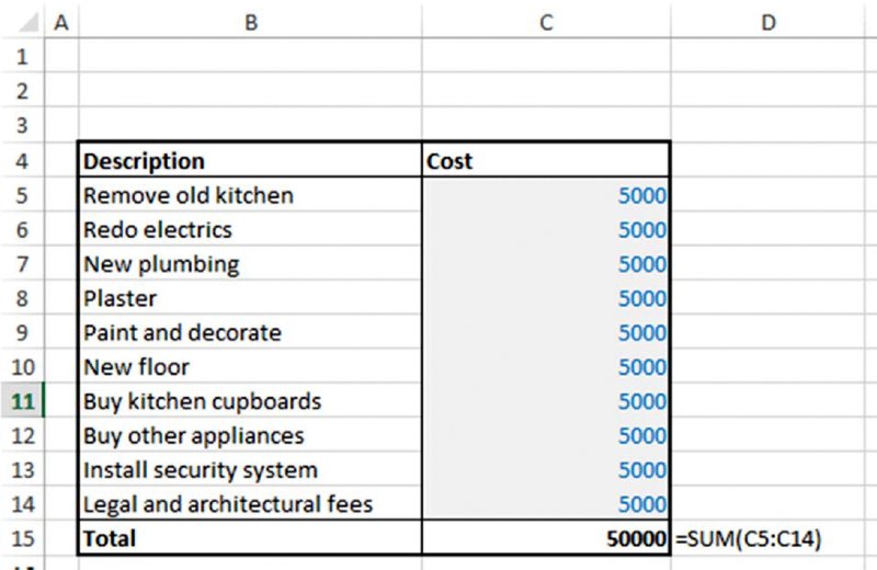
Figure 7.13 Cost Budget with Independent Items
The worksheet OneSource shows a modified model in which there is a common driver for all items; the model's formulae are adjusted appropriately to reflect this (see Figure 7.14).
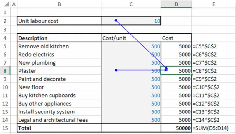
Figure 7.14 Cost Budget with a Common Driver
Note that the values in the range C5:C14 are still inputs to the model, and may now be able to be changed independently to reflect uncertainties in each that are not driven through the common factor.
7.4.2 Example: Scenario-Driven Variability
In Chapter 6, we mentioned that one use of general scenario approaches is to capture dependencies between items, and in particular to act as a proxy tool to capture dependencies that are difficult to express through explicit formulae (such as price–volume demand curves).
The file Ch7.PriceScenarios1.xlsx contains an example in which there are four possible scenarios for the future development of prices, each with its own periodic growth rate and starting value. Figure 7.15 shows the model in which a standard growth formula is applied to calculate the future time profile, but where the parameters for the growth formula (in cells D10 and E10) are established by using the CHOOSE function to pick out the appropriate values from the table of scenario data (cells D5:D8), based on the scenario number selected in cell C10.
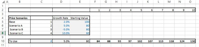
Figure 7.15 Scenarios for Price Development
In terms of the similarity between static modelling and risk modelling, it is of no relevance (from the perspective of the formulae required in the model) if the scenario number (cell C10) is set manually or by using a discrete probability distribution that returns a random integer between one and four. Figure 7.16 shows a multi-output DataTable, which contains the full price profile for each scenario (which is also contained in the example file). If the scenario numbers were chosen randomly, then the profile of price development would simply be a randomly varying selection between the four profiles.
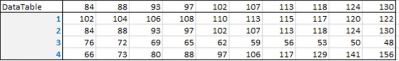
Figure 7.16 Price Development in Each Scenario, Using Sensitivity Analysis
7.4.3 Example: Category-Driven Variability
The assignment of items to categories can be an invaluable tool when building and communicating models.
From a modelling perspective, the use of categories may be relevant in several types of situations:
- It provides a more general way to capture sources of common variation (rather than a single one used in the above example). In other words, several risk items may be affected by one particular underlying risk driver, and other items by another, and so on.
- It can help to capture relationships between risk impacts (even where the occurrences are independent). For example, there may be a set of risks whose individual occurrence affects the volume produced (or sold) by a company of a particular product (and/or in a particular region), but where the total impact is only that of the largest one that has occurred. The use of categories allows Excel functions (such as SUMIFS or other conditional calculations) to capture the impact.
- As a method to group smaller item risks, so that those that are individually of little significance are not simply ignored.
From a communication and results presentation perspective, the use of categories can be an important tool: one may often wish to communicate results at a higher (more aggregate) level than the one that a project team is working at within its day-to-day risk assessment activities.
The file Ch7.Cost.HouseRenovation.Categories.xlsx contains an example. A detailed list of cost items for a renovation project is shown in the worksheet ListofCostItems; see Figure 7.17.
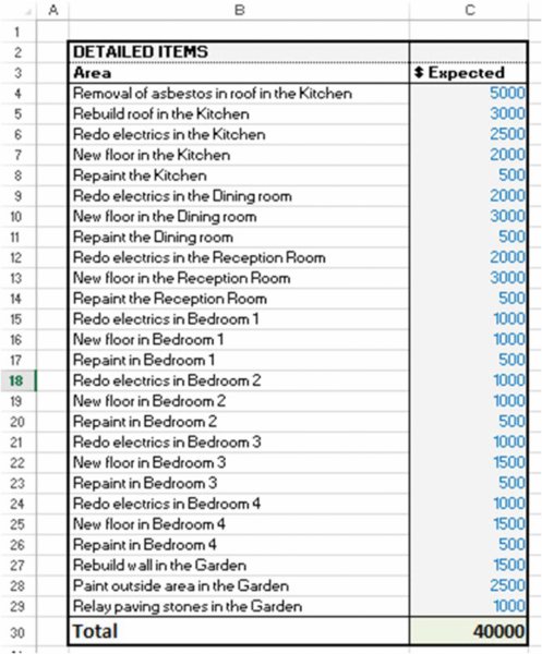
Figure 7.17 Detailed Cost Budget Without Categories
These items could be categorised by the area (room) of the house, and by the nature of the activity, as shown in the worksheet AggCategories of the same file; see Figure 7.18.
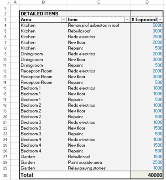
Figure 7.18 Detailed Cost Budget with two Types of Category
The data are effectively structured as a database that can be presented in summary form in different ways for reporting and communication purposes. Figure 7.19 shows the summary presentation by area (room) and by item (activity); in the example file, this is shown immediately below the table.
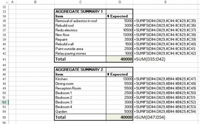
Figure 7.19 Summary of Cost Budget by Each Type of Category
It is important to note that the categories used for sensitivity and modelling calculations should correspond to the drivers of sensitivity or risk. Therefore, the choice of such categories is much more limited than it is for categories that may be desired for communication or presentation purposes (e.g. geographical region, department, responsible person, process stage, subtask, etc.).
The worksheet SensCategories of the same file (partly shown in Figure 7.20) contains a supposed categorisation for sensitivity and risk purposes, in which there are four categories (perhaps associated with the structure of the contractor relationships, for example); a summary of the cost structure by sensitivity group (risk drivers) is shown in Figure 7.21.
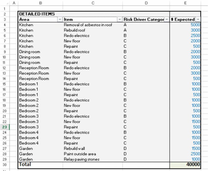
Figure 7.20 Detailed Cost Budget with Risk Categories
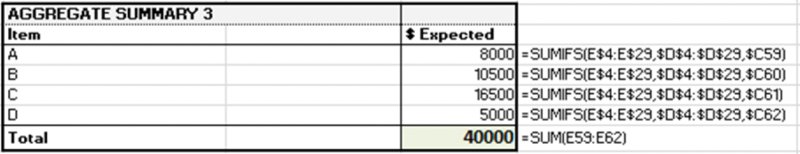
Figure 7.21 Summary of Cost Budget by Risk Category
One can then conduct a sensitivity analysis of the total cost by varying the ranges that apply for the different sensitivity categories or risk drivers: these calculations are contained in the worksheet SensCategoriesRanges; see Figure 7.22.
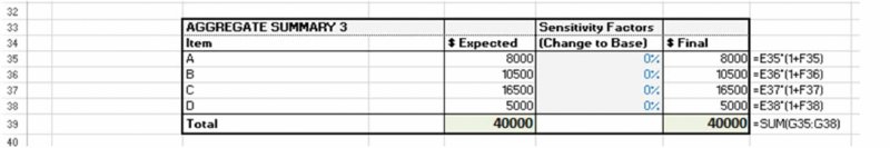
Figure 7.22 Sensitivity Analysis of Cost Budget by Risk Category
Note that the mechanism by which any subsequent variation is implemented (e.g. traditional sensitivities or random sampling) is essentially irrelevant from a modelling perspective. Figure 7.23 shows a DataTable as the sensitivity factors for the drivers A and B are varied.
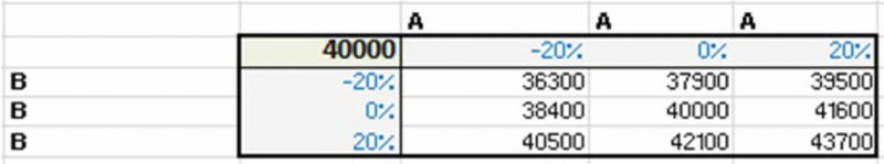
Figure 7.23 Sensitivity Analysis of Cost Budget for Two Risk Categories
Of course, the use of categories of risk drivers means that there is a smaller set of underlying risk drivers than if risks were treated as individual items; each category is implicitly a set of risks that vary together (or are jointly dependent). Clearly, this will affect the extent of variability at the aggregate level when a simulation is run.
The file Ch7.Cost.HouseRenovation.Categories.Comparison.xlsx contains an example in which two separate modelling approaches are implemented: in the first, the risks are independent items, and in the second, each risk is driven by a risk category. Figure 7.24 shows a screen clip of the two approaches, with Figure 7.25 showing an overlay of the simulated results. Clearly, the approach that uses categories has a wider range for the possible outputs; in the first case, it is more likely that some of the items offset each other (due to combinatorial effects), so that the range is narrower.
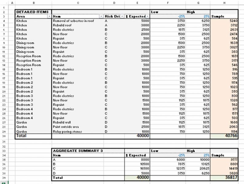
Figure 7.24 Uncertainty Model of Cost Budget by Risk Category
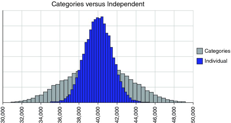
Figure 7.25 Simulated Distribution of Total Costs, Comparing Individual Independent Items Versus the Use of Risk Categories
Thus, although the use of great detail at the line item level can be important to capture all factors when working with static models, such detailed approaches may not be directly applicable to the creation of risk models; often, items need to be grouped into categories, with any variation driven at the category level (thus, involving the creation of intermediate calculations compared to the case where risks are treated as individual items only). In general, as a model becomes more detailed, there are more potential dependency relationships, because any item can theoretically interact with any other. Therefore, one of the modelling challenges is to build the risk drivers into the model at the appropriate level of detail.
Although the categories used for sensitivity and risk modelling purposes should correspond to the drivers of risk, one may wish to communicate the results of models according to other categories. In this example, this has been done by aggregating the results by risk driver (cells H35:H38) to create scaling factors by communication category (cells J35:J38); these show the amount by which the item in each category varies from its base case (in a particular sample or recalculation of the model). These factors are then applied to the detailed model (cells J4:K29), using lookup functions to find the scaling factors that apply for each individual item based on its category. The individual items are then summed by communication category (cells H44:H51), and these would also form a simulation output, if a simulation were done. (This approach is numerically equivalent to one in which the model was built by sampling the percentage scaling factor for each risk category and then applying that to the items within that category, before summing the figures according to communication category).
Figure 7.26 shows a screen clip of this, with the distribution of costs for the kitchen-related items. (The simulation is done using @RISK, in order to easily display the output graphically; a reader working with the model can run the simulation using the tools and template of Chapter 13, if desired, as the model formulae are created without using @RISK.)
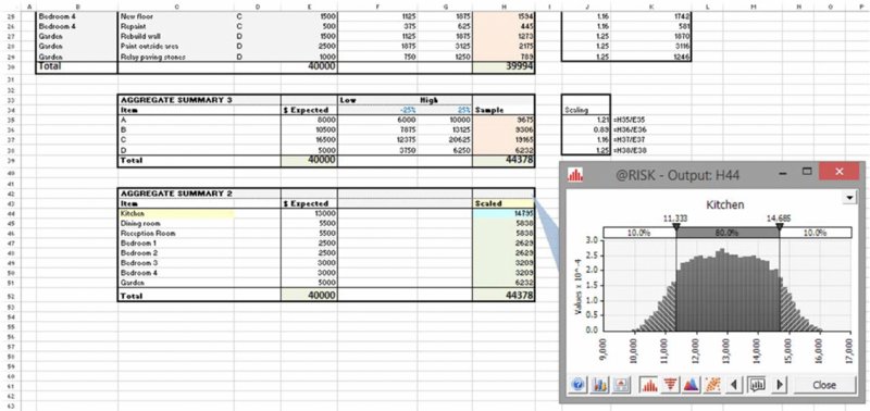
Figure 7.26 Simulated Distribution of Costs by Presentation Category
This example also shows that, in order to present the results of risk models in a particular way (i.e. in this case, by the category associated with the room type), additional work may be necessary to build the appropriate formulae; such issues should be taken into account as early in the process as possible, because the conducting of such rework only once results are being presented can lead to time shortages and errors, which can severely detract from the credibility of the results (and provide reinforcement to those who are sceptical about the benefits of such approaches).
7.4.4 Example: Fading Impacts
When considering the risks associated with the start-up phase of a new production facility, there may be a risk that it cannot immediately be operated at planned capacity, perhaps due to a lack of experience that a company has in producing identical products. More generally, the impact of a risk (if it materialises) may reduce over some period (which itself may be uncertain).
Note that the risk is in relation to a planned figure (i.e. a deviation from it), so that other planned items would, as a general rule, be part of the base plan and not considered as genuine risks, at least relative to a reasonable base plan. For example, there may be a ramp-up phase in which planned production starts below full capacity but then increases over time to full capacity, or that sales prices may initially be lower in order to attract new customers; the fact that the initial values are expected to be below their long-term equilibrium is not a risk as such.
The file Ch7.FadeFormulae.xslx contains some examples of possible implementations of the calculations for the loss of capacity (expressed as a percentage of the total), which decreases over time. A screen clip is shown in Figure 7.27.
- In Model 1, the figures are hard coded.
- In Model 2, there is a constant improvement per year, which is determined by the assumed starting and ending values over a fixed period of time (i.e. between period 1 and period 5 in this case).
- In Model 3, the end period to which improvements apply can be changed, with constant improvement per year, so that an additional check is built into the formulae to prevent values becoming negative in some cases.
- In Model 4, the end period can also be changed, but the improvements are applied in a relative sense, so that the loss of capacity is calculated in a multiplicative fashion from the prior period figure, until the end period is reached.
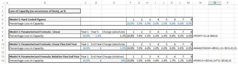
Figure 7.27 Various Possible Implementations of Fade Formulae
Of course, the advantage of Model 1 is that any figures can be used for the time profile (simply by typing in the desired figures); the other approaches have the advantages that the number of inputs is reduced, and that the conducting of sensitivity analysis is more straightforward.
Since the inputs to the formulae can be changed, such changes may either be sensitivity related or risk driven. For example, in Model 4, the percentage that applies in the first period could be replaced by a sample from an appropriate uncertainty distribution, as could the ending year and the annual relative change. The calculated capacity loss may also be used to represent the impact of a risk on its occurrence, and combined with the outcome of a sample from a “yes/no” (Bernoulli) process (see Chapter 9) by simple multiplication.
Similar approaches can be used if there are several potential risks that may interact. For example, in each period there may be a risk of a shock event to market prices. Where the impact of each shock may persist over several periods, then within each period, one would need to calculate the impact of all prior shocks whose effect is still applicable at that point. Such calculations would be similar to some of those shown in the next section.
7.4.5 Example: Partial Impact Aggregation by Category in a Risk Register
Relationships that are more subtle or complex than those discussed above can often arise. For example, one can envisage a situation in which a company has identified some initiatives to improve the efficacy of its sales processes, such as:
- Improved screening of customers, so that low potential leads are not followed.
- The reuse of bid documents, so that quotes can be provided at lower cost.
- Enhanced training of new sales representatives.
- The development of new products.
- A more systematic process to track competitor activities.
From a qualitative perspective, these initiatives would seem sensible and could presumably be authorised for implementation. On the other hand, it would be natural to ask whether these initiatives would be sufficient for the company to achieve its improvement targets; thus, some quantitative analysis would be required.
One could consider various quantitative approaches to this:
- Using a static approach, assess the impact of each initiative quantitatively (as a fixed improvement percentage) and add up these static figures.
- Using a static approach, attempt to reflect that the effect of subsequent initiatives is reduced (compared to its stand-alone value) as other initiatives take effect. One could think of a number of possibilities (described in more detail in the example model):
- A multiplicative diminishing effect.
- A weighting effect, in which the largest initiative is fully effective, the second one is less effective, and so on.
- A risk approach, in which the success of each initiative (and more generally its impact) is uncertain.
The file Ch7.ImprovInit.Effect.xlsx contains various worksheets that show possible calculations for each case. It aims to demonstrate that the core challenge is to identify and build the appropriate aggregation formulae. Once this has been done, the mechanism by which input assumptions are changed (sensitivity analysis or random sampling) is not of significance for the formulae. Figure 7.28 shows the static case, where the effect of the initiatives is added up (shown in the worksheet Additive).
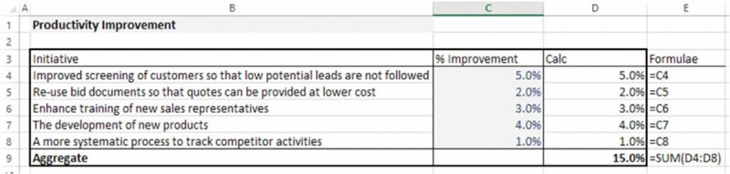
Figure 7.28 Approaches to Aggregating the Effect of Improvement Initiatives: Addition of Static Values
Figure 7.29 shows the situation where it is believed that there is a diminishing cumulative multiplicative effect (shown in the worksheet Multiplicative).
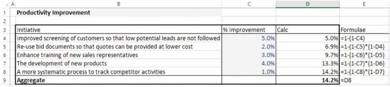
Figure 7.29 Approaches to Aggregating the Effect of Improvement Initiatives: Multiplication of Static Values
Figure 7.30 shows the case where the initiative with the largest effect has its effect included with a 100% weighting, the second with a 50% weighting (of its base stand-alone value), and so on; in order for the model to be dynamic as the input values for the base improvement percentages are changed, the LARGE function is used to order the values of the effects of the initiatives (shown in the worksheet SortedWeighted).
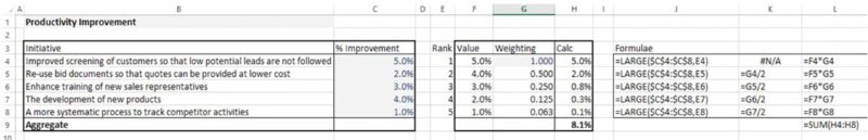
Figure 7.30 Approaches to Aggregating the Effect of Improvement Initiatives: Weighting Factors of Static Values
Note that whichever of the three approaches is deemed appropriate (the reader may be able to think of others), the final step – of adding risk or uncertainty for the percentage improvement figures – is straightforward. The worksheet SortedWeightedRiskRAND (Figure 7.31) contains the case where each initiative has a probability of success (using the RAND() function within an IF statement), and the worksheet SortedWeightedRiskAtRisk (Figure 7.32) shows the equivalent using the RiskBernoulli distribution in @RISK, as well as a graphic (using @RISK) of the simulated distribution of improvement percentage.
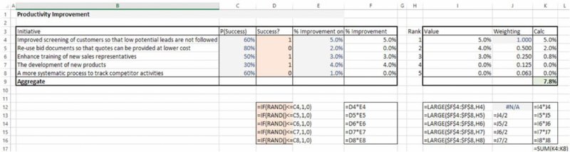
Figure 7.31 Approaches to Aggregating the Effect of Improvement Initiatives: Uncertainty Ranges Around the Selected Static Approach (Excel)
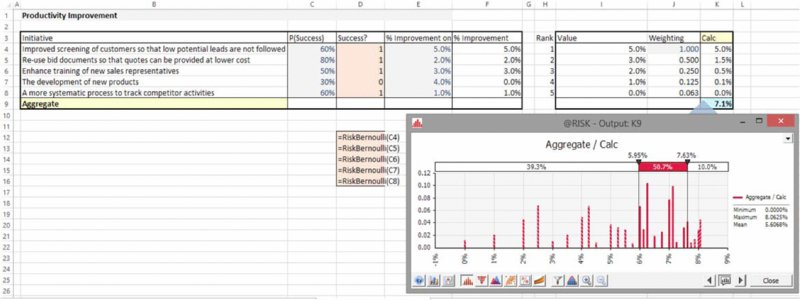
Figure 7.32 Approaches to Aggregating the Effect of Improvement Initiatives: Uncertainty Ranges Around the Selected Static Approach (@RISK)
7.4.6 Example: More Complex Impacts within a Category
When working with categories, one may need to be able to find the minimum or maximum value within a category. Whereas Excel contains functions such as SUMIF, SUMIFS, AVERAGEIF, AVERAGEIFS, and so on, it does not (at the time of writing) have a MAXIFS or MINIFS function. Whereas SUMIF or SUMIFS can be replicated using array functions, the analogous formulae for maxima and minima would not work in general. The AGGREGATE function can be used instead (although it is available only in later versions of Excel). The key is to use the function option, which ignores errors (i.e. with its Options parameter set to the value 6), and to calculate it as an array function in a way that its elements create errors when a criterion is not met, so that only items meeting the criteria are included within the calculation.
The file Ch7.MaxIfs.Aggregate.Array.xlsx contains an example; a screen clip is shown in Figure 7.33. Whereas the maximum of the (positive) revenues can be calculated using an array form of the MAX function (e.g. using the formula {=MAX((D$3:D$18)*($C$3:$C$18=$G4))}), such a formula would not work for the (negative) cost field (see columns H and I, respectively). However, by using the AGGREGATE function in an analogous way (using division to create an error if the criteria are not met, and ignoring this error through the function's option 6), one can create a formula that could find the maximum or minimum of any set of numbers, whether positive or negative, as shown in columns J, K and L.

Figure 7.33 Working with Only the Maximum Impact Within a Category
7.5 Working with Existing Models
When building a risk model in practice, very often one has an existing model, populated with base case numbers, as well as perhaps some sensitivity or scenario analysis that has been conducted. A frequent issue is therefore whether, and how, such models can be used as the basis for the creation of risk models. Indeed, a project team may sometimes be charged with the task of “adding risk” to the existing model.
In this section, we discuss the issue of the design of risk-based simulation in such circumstances. This section is not intended to be complete by itself, as the building of models requires techniques and processes that are mostly covered earlier. The discussion here highlights only selected key points. Indeed, some issues are not covered again at all below, such as the use of model switches to be able to capture the effect of key project decisions and mitigation actions.
7.5.1 Ensuring an Appropriate Risk Identification and Mapping
From the earlier discussion, it is clear that one can, in principle, take (almost) any well-built existing static model and replace the fixed input assumptions with distributions, thus creating an uncertainty model that can be repeatedly recalculated. On the other hand, such an approach is unlikely to result in a risk model that is genuinely appropriate, due to issues mentioned earlier:
- The line items are unlikely to match the risks; significant model restructuring would generally be necessary, both to provide the granularity required and to include the impact of event risks or other items.
- The formulae are likely to be insufficiently flexible, especially concerning delay-type risks, which are rarely built into static models (unless detailed thought was given to model requirements early in the process).
- Dependencies between items may have been overlooked, especially common drivers of risk, or relationships may only take effect in more complex scenarios of multiple input variation.
Of course, with sufficient restructuring, any existing model can be adapted (or essentially completely rebuilt) to include the risks and their impacts. However, as a general rule, the effort required to do so (correctly) is often extensive. Indeed, the potential complexity in restructuring an existing model is one of the reasons why “overlay” models, such as risk registers, are frequently used.
Of course, such restructuring activities will be minimised if one can consider the risk issues early in the model design process: thus, as well as considering “What-if?” sensitivities at this stage, one would ideally also begin to consider the likely key risks and their impact for model design. A frequently observed case is essentially the extreme opposite, where an analyst spends perhaps several weeks or months building a detailed static model, without considering risks, and then finds that the effort required to modify the model to incorporate the results of a risk assessment is so extensive that it is never undertaken.
7.5.2 Existing Models using Manual Processes or Embedded Procedures
There may be cases where an existing static model is believed to be appropriately structured to be suitable directly for risk modelling purposes, in the sense that simple replacement of its input values with the appropriate probability distribution would lead to a model with a valid risk mapping (and not simply to a model that produces no calculatory errors, but whose scenarios shown are not realistic cases, with, for example, inappropriate line items, as discussed earlier).
In some cases, models require other (non-simulation) procedures to be run, some of which may (for a static model) be run manually, and others may involve automated (macro) procedures. Examples include:
- Before and after a simulation, to ensure that model switches are automatically set to their appropriate values; so that the model's presentation (when a simulation is not running) is always of the base case, with the “risk case” used automatically whenever a simulation is run.
- Before a simulation, to ensure that Excel Data Filters are cleared on databases, so that the integrity of the calculations (and of the filtered display) is maintained.
- Before a simulation, to refresh the input data by updating some values taken from an external data source of worksheet (or similarly to write simulation results to an external database at the end of a simulation).
- Before or after a simulation, a GoalSeek or Solver procedure might be used to find or optimise the values of other model inputs.
- During a simulation, some procedures may need to be run at each iteration (recalculation) of it. This may include:
- GoalSeek or Solver. For example, for every sample of an exchange rate, one may wish to know what the target sales price should be to achieve breakeven, or to find an optimal selling price. These would be items that would be determined if that specific case arose in the real-life situation, and so need to be reflected within the simulation.
- Circular references. These are usually resolved by iterative means (where they have not arisen by mistake, or can be eliminated by algebraic manipulation or model reformulation). There are two main iterative approaches used: first, Excel's iterations option (using the Enable iterative calculation within the Excel Options/Formulas) and second, the creation of a “broken” calculation path within Excel, so that (for a particular variable on the circular path) its prior calculated values are contained in one set of cells, and its updated values are contained in another adjacent set. The updated values are pure values (not formulae), which feed all model calculations (including the calculations of the prior values), but there is no formula link from the prior value to the updated ones; rather a macro is used to iteratively assign (copy) the values from the (calculated) prior field into the (pure) values of the updated field until the difference between the two is close to zero.
- A model may contain DataTables that, by default, update automatically at each iteration, but whose values are only relevant in the static (base view).
- A bespoke macro or other procedure may be required whenever inputs change. For example, once the geographic area to be focused on is decided, then a database (or another workbook) needs to be consulted in order to find the model values that apply for that geography.
The principles of dealing with such cases are as follows.
First, for procedures that are required only before or after a simulation, these can be either:
- Run manually at the appropriate time, as they would have been if working with the model without running a simulation; or
- Encoded within a macro that is embedded within the overall simulation (i.e. automatically run either at its start or at its end).
Second, procedures that need to be run each time that input values change (i.e. at each iteration or recalculation of the simulation) must be encoded within a macro that is embedded within the simulation. The key points in this respect are:
- The core challenge is to ensure the integrity of the calculations; many procedures (including some formatting operations) would cause Excel to recalculate as the procedure is running, so that distributions are resampled. This would create not only a slower simulation but also a potential lack of integrity of the calculations: the initially recorded values of input distributions may not correspond to the actual values used in the final calculation, or iterative procedures may never find a solution, as their target value changes as the procedure is being run.
- The solution is to ensure that the distribution samples are “frozen” whilst such procedures are running (at each recalculation or iteration of the main simulation loop). The implementation of such “freezing” procedures is different in Excel/VBA than it is in @RISK, and also varies according to the version of @RISK used. Therefore, the details of the discussion are contained within the individual chapters devoted to each topic (i.e. Chapters 12 and 13).
The remainder of this chapter provides a number of examples of encoding macros to turn manual procedures into automatic ones; these apply to procedures that need to be run before and/or after a simulation, but not during it. (The examples, of course, all use macros; Chapter 12 provides an introduction to macros for readers who have little experience of the subject.)
7.5.3 Controlling a Model Switch with a Macro at the Start and End of a Simulation
The file Ch7.BaseSwitch.Macro.xlsm contains an example in which macros are used to switch between the base and risk cases, by clicking on the corresponding button (i.e. a text box, with the associated macro assigned to it). This is shown in Figure 7.34. In practice, the macros could be run automatically (rather than manually using the button) by calling the MRSwitchtoRisk macro immediately before the start of a simulation, and then calling MRSwitchtoBase at the end.
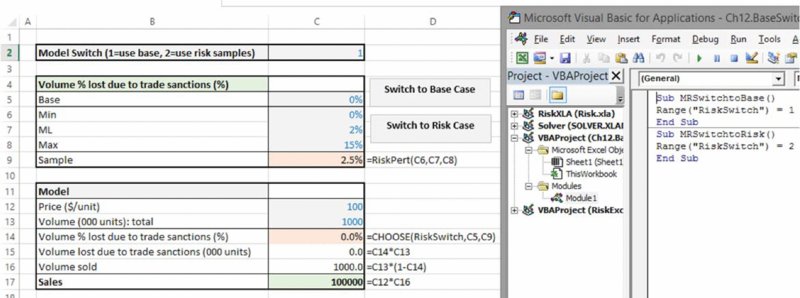
Figure 7.34 Controlling a Model Switch with a VBA Macro
The macros are contained within a new code module that was inserted in the VBA Window, and the code for each is:
Sub MRSwitchtoBase()
Range("RiskSwitch") = 1
End Sub
and
Sub MRSwitchtoRisk()
Range("RiskSwitch") = 2
End Sub
Note that (as covered in more detail in Chapter 12), it is more robust to refer to Excel cells from VBA using named ranges rather than cell references, which is why cell C2 has been given the name RiskSwitch within the Excel worksheet.
7.5.4 Automatically Removing Data Filters at the Start of a Simulation
Whereas the above macros were very simple to write directly, in other cases one may need to record the process steps in order to create a macro. This is typically the case when procedures that are more complex than just changing the value in a single cell are required.
An important case is to ensure that any Data/Filters in Excel are not in operation when a simulation is run. Some models (especially for cost budgets and portfolios of projects) are structured as data sets, and the use of filters is highly convenient to display subcategories of items using a drop-down menu. On the other hand, the values shown by the filters or the calculations can be incorrect or unexpected if the filters are active as risk values are updating. Thus, one should generally remove filters before a simulation is run. To ensure that this is not overlooked, one may encode their removal in a macro that is embedded within the simulation, so that it is run automatically immediately before the main recalculation loop of any simulation.
One can record a macro of the steps of removing a filter (by using Developer/Record Macro, removing the filter, and then using Developer/Stop Recording). When removing the filter, the Excel toolbar or the short-cut Alt+D+F+S can be used. After doing so, the code would have been inserted into a new module within the VBE:
Sub ClearAllFilters
ActiveSheet.ShowAllData
End Sub
One may generalise the code in certain ways, such as to use On Error Resume Next so that the code runs without stopping if no filters are active. For example, slightly more general code would be:
Sub ClearFilters()
On Error Resume Next
With SheetContainingtheFilters
  .Activate
  .ShowAllData
End With
End Sub
Further generalisation could include the case where there are filters on multiple worksheets of the workbook, in which case one can apply the above procedure to each worksheet by working through all worksheets in a workbook using a For Each…In loop that is also used in Chapter 12.
The file Ch7.Filter.xlsm contains an example, as shown in Figure 7.35.
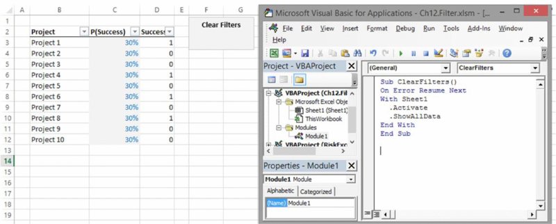
Figure 7.35 Clearing Filters with a VBA Macro
The principles of recording code (before perhaps adapting it) would also apply when other more complex syntax would be necessary, such as when using GoalSeek or Solver. In essence, one would again need to record the step of running the code once. One subtlety is that when using code that results from recording a run of Solver, a True statement needs to be added in order for the macro to completely run to the end. Thus, one may record code such as:
SolverOk SetCell:="$G$3", MaxMinVal:=1, ValueOf:="0",
ByChange:="$D$5:$F$5"
    SolverSolve
whereas the required code would need to end with:
SolverSolve True.7.5.5 Models with DataTables
In general, DataTables are almost always only required when the model is in the static or base case view. On the other hand, they will be recalculated at each iteration (recalculation) of a simulation, and hence slow down the simulation (switching off the automatic recalculation of DataTables using Excel/Options will not change this, as the simulation forces a workbook recalculation). There are a number of options available to deal with this:
- Deletion or clearing. In some cases, the use of DataTables is a first step in a process of sensitivity analysis, which ends in a decision to build a full simulation model; in such cases the tables may no longer be relevant. As a variation, one may instead clear out only the content of the ranges containing array formulae within the DataTables, in order to retain their basic structure and formatting, allowing them to be reimplemented quickly if needed.
- Placement in another worksheet whose recalculation is turned off during the simulation run, so that the DataTables will not be unnecessarily recalculated. The procedure to switch off the recalculation of a worksheet requires VBA code that is explained in Chapter 12. In a sense, this approach is the most robust and transparent, as it ensures user control of the calculation process. The main complexity is that a DataTable can only vary input values that are in the same worksheet, so the base values would need to be in such a worksheet.
- Using macros to create a replacement for a DataTable. In this approach, a macro is used to sequentially assign (from a predefined list) the values to be used for a model's input and each time a new value is assigned, the model is recalculated and the results recorded. This “sensitivity” macro could therefore be run separately to the simulation, and is shown in the following example.
The file Ch7.RevSensitivity.xlsm provides an example of the use of a macro to replace a DataTable, and is shown in Figure 7.36. The macro sequentially places the values for revenue growth (from the cells below the header I12) into the cell corresponding to the relevant model input (cell E4) and recalculates the model before recording the result (contained in the cell J9) in the corresponding cell (below the header J12).
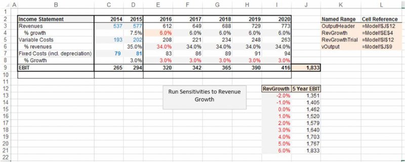
Figure 7.36 Running Sensitivities with a VBA Macro
The appropriate cells that are involved in the operations (or serve as reference points for finding the input values to use and to store the results) have been given named ranges in Excel. The code is:
Sub MRRunSens()
N = Range("RevGrowthTrial").CurrentRegion.Rows.Count
For i = 1 To N - 1
 Range("RevGrowth") = Range("RevGrowthTrial").Offset(i, 0)
 Application.Calculate
 Range("OutputHeader").Offset(i, 0) = Range("vOutput")
Next i
End Sub
Note that in the context of a simulation model, in which the actual input cell to the model is a CHOOSE function that selects either a base value or a risk value, the above code would be used to place the desired input values into the cells originally containing the base value (which then feeds into the model via the CHOOSE function if the model switch is set to show the base case). In more general cases, the macro would work through a set of integers, which drives a lookup function to replace several model inputs at the same time, as discussed in the scenario approach in Chapter 6.