
3Typical Chaotic Systems
Chaos exists widely in nature. During the research and development of chaos theory, researchers found a lot of chaotic dynamics models, and some of them are typical for the chaos theory and application research, including discrete-time chaotic maps, continuous-time chaotic systems, and hyperchaotic systems. In this chapter, we will discuss the mathematical model and its main characteristics of some typical chaotic systems.
3.1Discrete-Time Chaotic Map
First, the definition of discrete-time chaotic map is presented. Consider a nonlinear system
where “○” represents a compound operation between two functions. x(k) ∈M⊂ R, u(k) ∈ RP, {Gu}u∈RP is the diffeomorphism group with p parameters on M. F:M → M is a diffeomorphism. If x(k) is chaotic, and x0 ∈M, then we call x(k), which all pass through x0 on smooth n-dimensional manifold M, is discrete chaos. The physical meaning is that chaos is generated by a discrete map described by a nonlinear difference equation, which can usually be achieved by a software program or sampler.
3.1.1Logistic Map
Logistic map is the most widely used discrete chaotic map model, and its equation is [4]
where the parameter μ ∈ (0, 4] and xn ∈ (0, 1). When 3.5699 . . . < μ ≤ 4, it is chaotic. The dynamical state of the system changes with the system parameter, which includes the following aspects:
- When μ ∈ [0, 1], the system has a fixed point xn → 0.
- When μ ∈ [1, 3], the system has fixed points xn → 0 and xn → 1 – 1/μ. This is called period 1 solution.
- When μ ∈ [3, μ′), μ′ = 3.569945672 . . ., where orbital period changes such as 1 → 2 → 4 → 8 . . . occur. This is called period-doubling bifurcation phenomenon.
- When μ ∈ [μ′, 4), the system shows a chaotic phenomenon.

Figure 3.1: Bifurcation diagram of Logistic map.

The bifurcation diagram of the system is shown in Figure 3.1. The iterative initial value of x0 is 0.6, and the iteration number N is 2,000. The step size of μ is 0.01. As shown in Figure 3.1, when time series experiences four stages of evolution, from stable fixed point, unstable fixed points, period to chaos, complexity of the system increases. If μ = 4.0, the complexity is largest, which is shown in Figure 3.2 by the Lyapunov exponent. When μ = 4.0, Lyapunov exponent is equal to 0.69, which is the maximum.
Next, we will discuss the statistical properties of Logistic map.
The probability density function of Logistic mapping system is

The average value is
The autocorrelation function is
The cross-correlation function is
The advanced Logistic map, which is also called improved logistic map, is
The probability density function is

The average value is
The autocorrelation function is
The cross-correlation function is
3.1.2Tent Map
Tent map is another commonly used discrete chaotic map. The chaotic sequence generated by the tent map has been widely applied in the field of chaotic spread spectrum communication, chaotic encryption system, chaotic optimum algorithm, and so on. Its equation is
where the system parameter q ∈ (0, 1) and the variable xn ∈ (0, 1). Tent map and logistic map are topological conjugates. When q varies as (0, 1), the system is chaotic. In particular, when q = 0.5, the system is in a short-cycle state, such as (0.2, 0.4, 0.8, 0.4). In this case, the system is simple and its complexity is small. Therefore, for the application of tent map system, we should choose reasonable system parameter and initial value. Tent map system has the following statistical properties.
The average value is
The autocorrelation function is
The cross-correlation function is
3.1.3Hénon Map
Hénon map is a two-dimensional discrete chaotic system, which was proposed by Hénon in 1976. The map equation is [76]
When 1.07 ≤ a ≤ 1.4 and b = 0.3, it is chaotic. The variable xn ∈ (–1.5, 1.5). When a = 1.4, the complexity of the system is largest. Generally, in the study of the chaotic synchronization and encryption, we choose a = 1.4 and b = 0.3. The strange attractor of Hénon map system is shown in Figure 3.3, which looks like the galaxy in the sky, where the initial value xn(0) = yn(0) = 0.5, and the iteration times are 1,000. When b = 0.3, and a ∈ [0, 1.5], the bifurcation diagram of Hénon map system is shown in Figure 3.4. Obviously, it enters into chaos by period-doubling bifurcation.

Figure 3.3: Strange attractor of Hénon map.

3.1.4Tangent Delay-Ellipse Reflecting Cavity System Map
In 2004, Sheng et al. proposed a discrete chaotic system based on tangent delay (TD), which is called as TD-ellipse reflecting cavity system (TD-ERCS) map [77]. The map equation is

where the system parameter μ ∈ (0, 1], and the variables |xn| ≤ 1 and |yn| ≤ 1. m is an integer, which represents the number of TD. ![]() is the ellipse tangent slope after delaying m. k0 is determined by incident angle α, and the method is as follows.
is the ellipse tangent slope after delaying m. k0 is determined by incident angle α, and the method is as follows.
First, we calculate y0 and the slope of ![]() through the initial value x0 and system parameter μ
through the initial value x0 and system parameter μ

Then according to trigonometric function, we can obtain:
So, if we know the system parameters μ and m, and the initial values x0 and α, we can get the chaotic sequence {xn, kn}. When the TD m=0, the system becomes ERCS map. When m ≥ 1, the TD-ERCS is chaotic.
With the change in system parameter μ, the largest Lyapunov exponent of the system is shown in Figure 3.5. Because the curve chart looks like a flying goose, it is called “Goose.” The iteration number n is 400,000. Obviously, when μ = 1, the maximum Lyapunov exponent LE = 0.92. When μ = 0.5, the maximum Lyapunov exponent LE = 0.33. Thus, the maximum Lyapunov exponent is greater than zero in the range of μ, which shows that TD-ERCS is chaotic in the whole range.
When m = 1, there exists a square attractor for TD-ERCS as shown in Figure 3.6, where we choose μ = 0.8123, x0 = 0.7654, α = 0.9876, and the iteration number N is 1,500. At the beginning, the phase points are not on the attractor, but with the increase of iteration, phase points will fall on the attractor. The experiment also shows that if 0 < μ < 1, the position of square attractor is unchangeable and has no relation with the initial value. When μ = 1, the position of attractor is related to the initial values, but all phase points are on the attractor.

Figure 3.5: Maximum Lyapunov exponent of TD-ERCS system (x0 = 0.7654, α = 0.9876).

3.2Continuous-Time Chaotic System
First, we present the definition of continuous-time chaotic system. Consider the nonlinear system
where x(t) ∈ M ⊂ Rn; it is an integral curve through x0 in the vector field of F. x0 ∈ M and μ ⊂ RP are parameter vectors. If x(t) is chaotic, all x(t) going through x0 on the smooth n-dimensional manifold M are continuous chaos. From physical meaning, a continuous chaotic system is a nonlinear dynamical system and can produce chaotic phenomenon, which is described by the differential equation ẏ = F (x) and usually can be realized by analog circuit.
There are two types of continuous chaotic systems. One is autonomous system, such as the Lorenz system, Rössler system, and Chua system. The other is nonautonomous system, such as Duffing oscillator and van der Pol oscillator.
3.2.1Duffing Oscillator
Duffing oscillator is a typical forced vibration nonlinear dynamic system, and it belongs to nonlinear vibration problem. The Duffing system equation is [78]
where k is damping coefficient, f(x) is a nonlinear function, and e(t) is the drive term with period T. When f(x) and e(t) take different forms, we will get Duffing equation with different forms. Here, consider the following Duffing equation:
where k is the dissipative coefficient, and F and ω are amplitude and frequency of the periodic force, respectively. It is an important type that can generate chaos in nonlinear vibration.
Let ẋ = y, then eq. (3.23) is translated into
When k = 0, F = 1.5, and ω = 1, the attractor of the system is shown in Figure 3.7.

Figure 3.7: Chaotic attractor of Duffing system in x–y plane.

3.2.2van der Pol Oscillator
In 1926, van der Pol proposed a nonlinear nonautonomous system that is driven by external force, and the equation is [79]
When parameters b = 3, A = 5, and Ω = 1.788, the chaotic attractor of the system is shown in Figure 3.8.
3.2.3Lorenz System
When American meteorologist Lorenz investigated atmospheric convection model, he summarized a three-dimensional equation and found “butterfly effect,” which lays a foundation for chaos research. For Lorenz system, the mathematical model is a three-dimensional one-order nonlinear differential equation with three parameters, and it becomes one of the most typical examples to study chaos theory and its applications. Lorenz system has abundant bifurcation and chaotic phenomenon.
Lorenz system equation is [2]

where 3, r, and b are the system parameters. The third-order ordinary differential equation is based on the simplified model of heat fluid convection movement between the infinite flats. Its variables do not contain time, so it is called autonomous equation. x represents convection strength; y represents the temperature difference between upflow and downflow between the units; z represents the nonlinear intensity in the vertical temperature distribution; r represents the ratio of driving factors and inhibited factor that causes convection and turbulent, which are the main control parameters of the system. 3 = v/k is Prandtl value (where v and k are molecular viscosity coefficient and heat transfer coefficient, respectively); b represents the ratio of shape that is related to convection in aspect ratio; and 3 and b are dimensionless constant values.

Figure 3.9: Chaotic attractor of Lorenz system in x–z plane.
Numerical results show that when 3 = 10, b = 8/3, and 28 ≤ r < ∞, except some values near b (such as b = 100, 160, 260, and so on), the Lorenz system is in a chaotic state. Let 3 = 10, r = 28, and b = 8/3 and take numerical simulation for the Lorenz system, we get the famous attractor – “butterfly,” as shown in Figure 3.9. The butterfly attractor has two fixed points, and the orbit line transfers randomly around the two fixed points and forms the spiral shape, just like two wings of a butterfly.
3.2.4Rössler System
Rössler equation looks like the Lorenz system equation, but only a nonlinear term, which is also one of the typical systems in chaotic application research.
Rössler system model is described as [80]

where a, b, and c are system parameters. When a = b = 0.2, c = 5.7, the system is in a chaotic state. The Lyapunov exponent spectra are (0.0714, 0, –5.3943). The movement of the attractor describes the complexity of the system. The attractor of Rössler system is shown in Figure 3.10.

Figure 3.10: Chaotic attractor of Rössler system in x–y plane.
3.2.5Chua’s Circuit
In 1983, Professor Chua designed the famous nonlinear chaotic circuit at the first time, which is called as Chua’s circuit. Not only it can generate the rich and complex dynamic behaviors, but also the structure of the circuit is relatively simple. It has become a classical chaotic system for application of chaos control and chaos secure communication. It can produce period-doubling bifurcation, single-scroll, period 3, double-scroll attractor, and other complex nonlinear dynamic behaviors by adjusting the circuit parameters. On the basis of Chua’s circuit, the study of multi-scroll Chua’s chaotic attractors has become a research hotspot at present.
The normalized state equation of Chua’s circuit is [15]
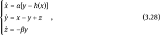


where h(x) is a piecewise linear function, and its waveform is shown in Figure 3.11. When h(x) is a different piecewise linear function, the system produces double-scroll and multi-scroll chaotic attractors. For chaos secure communication, the more the scroll is, the more secure the chaotic secure communication system is. Here only the double-scroll, three-scroll, five-scroll, and seven-scroll chaotic systems are simulated.
3.2.5.1Double-Scroll Chaotic Attractor
For double-scroll attractor, h(x) and other parameters are defined by

By Matlab simulation, we obtain the chaotic attractor as shown in Figure 3.12.
3.2.5.2Three-Scroll Chaotic Attractor
For three-scroll chaotic attractor, h(x) and other parameters are defined by


Figure 3.13: Nonlinear curve and the three-scroll chaotic attractor (a), (b) nonlinear curve; (c), (d) The three-scroll chaotic attractor in x-y plane.
Through Matlab simulation, the nonlinear function and three-scroll chaotic attractor are shown in Figure 3.13.
3.2.5.3Five-Scroll Chaotic Attractor
For five-scroll chaotic attractor, h(x) and other parameters are given by

By Matlab simulation, the five-scroll chaotic attractor is shown in Figure 3.14
Figure 3.14: Five-scroll chaotic attractor: (a) Parameter 1 (x–y plane) and ( b) parameter 2 (x–y plane).

3.2.5.4Seven-Scroll Chaotic Attractor
For seven-scroll chaotic attractor, h(x) and other parameters are described as

Through Matlab simulation, the seven-scroll chaotic attractor is shown in Figure 3.15.
3.2.6Chen System
In 1999, in the research of anti-control of chaos, Professor Chen discovered a new chaotic attractor. From the phase diagram of the system, compared with the “butterfly” attractor, it is more complicated on the phase space.
The mathematical model of Chen attractor is [16]

where X = (x, y, z)T ∈ R3 is the state of the system; a > 0, b > 0, and c > 0 are the system parameters. Although Chen system is similar to the other two famous chaotic systems – Lorenz system and Rössler system in the form, Professor Chen proved that it isn’t topological equivalence with the two chaotic systems. The attractor of this system is different from any previous chaotic attractors, and qualitatively analysis the features of the attractor, such as bifurcation, the route to chaos. If a = 35, b = 3, and c = 28, the strange attractor of Chen chaotic system is shown in Figure 3.16.
Hardware circuit of Chen system is designed and tested in Ref. [81], and the circuit diagram and experimental results are shown in Figures 3.17 and 3.18, respectively. Obviously, the experimental results are consistent with the simulation results.
3.2.7Lü System
In 2002, Lü and Chen discovered a new chaotic attractor, which connects the famous Lorenz attractor and Chen attractor. The mathematical model of Lü system is [82]

Figure 3.16: Phase diagram of Chen’s chaotic attractor in x–z plane.


where a, b, and c are system parameters. When a = 36, b = 3, and c = 20, the system is in a chaotic state. The chaotic attractor of the system is shown in Figure 3.19.

Figure 3.19: Attractor of Lü system in x–z plane.
3.2.8Unified Chaotic System
In 2002, Lü and Chen proposed a new chaotic system, and the system connects the Lorenz attractor and Chen attractor. Lü system is just a special one of the new chaotic system, so it is called the unified chaotic system. According to the definition of Vanĕ^ček and Čelikovský [83], Lorenz system, Chen system, and Lü system belong to different topology types. Mathematical model of the unified chaotic system is [84]

where the system parameter α varies in the interval [0, 1]. At this range, the unified chaotic system has full chaotic characteristics. According to the definition of Vanĕ^ček and Čelikovský [83], when α varies in the interval [0, 0.8), the unified chaotic system belongs to the generalized Lorenz system. When α varies in the interval (0.8, 1], the unified chaotic system belongs to the generalized Chen system. When α = 0.8, the unified chaotic system belongs to Lü system. So the unified chaotic system plays an important role in connecting Lorenz system with Chen system, and it is a one-parameter continuous chaotic system. Namely, using only one parameter α, we can control the entire system. When α gradually increases from 0 to 1, the system also gradually transits from the generalized Lorenz system to the generalized Chen system [85]. Under the different parameters of unified chaotic system, the chaotic attractors in the x–z plane are shown in Figure 3.20. The unified chaotic system parameter α has the largest Lyapunov exponent in the range of [0, 1] as shown in Figure 3.21, except the three obvious periodic windows, W1 = [0.369, 0.371], W2 = [0.468, 0.470], W3 = [0.575, 0.597]. The largest Lyapunov exponent is greater than zero in the range of [0, 1], so the unified chaotic system has full chaos characteristics. Due to its excellent performances, the control and synchronization of the system become a hot topic for the chaotic research [86], and it has extensive application prospect in the field of secure communications [87].

Figure 3.20: Attractors of unified chaotic system with different parameters in x–z plane. (a) α = 0; (b) α = 0.5; (c) α = 0.8; and (d) α = 1.


3.2.9Simplified Lorenz System
Dynamic equation of simplified Lorenz system is [56]

where c is a bifurcation parameter of the system. The maximum Lyapunov exponent of simplified Lorenz system is shown in Figure 3.22. When c ∈ [–1.59, 7.75], the system is in a chaotic state obviously. But there exists nine period windows in this range at least, namely, W1 = [3.507, 3.509], W2 = [4.581, 6.612], W3 = [4.6911,4.722], W4 = [5.122, 5.127], W5 = [5.167, 5.169], W6 = [5.599, 5.600], W7 = [5.7601,5.770], W8 = [5.820, 5.830], and W9 = [6.415, 6.425].
With the change of the system parameter c, the bifurcation diagram of the simplified Lorenz system is shown in Figure 3.23. The chaotic attractor of the simplified Lorenz system is shown in Figure 3.24.
Simplified Lorenz system has the following properties:
- It is chaotic over most of the range c ∈ [–1.59, 7.75].
- For c = –1, it is the usual Lorenz system with the standard parameters.
- For c = 0, the variable y is removed from the second equation.
- For c = 6, the variable x is removed from the second equation.
- There is a rich set of bifurcation as c is varied over the range.
- According to the topological definition by Vanĕ^ček and Čelikovský [83], the linearization of system (3.36) about the origin produces a 3 × 3 constant matrix of partial derivatives, A = [aij]3×3, in which the sign of a12a21 distinguishes nonequivalent topologies. According to this criterion, when c < 6, a12a21 > 0; when c = 6, a12a21 = 0; and when c > 6, a12a21 < 0.

Figure 3.23: Bifurcation diagram of the simplified Lorenz system.

Simplified Lorenz system can be implemented by analog circuit. The nonlinear part uses operational amplifier LM741 and multiplier AD633 to implement. According to the simulation, the variable amplitude exceeds the voltage range that operational amplifier and multiplier provide, so the system state variables cannot be directly as the voltage variables. To realize the circuit systems, the state variables must be scaled for transformation appropriately. Simplified Lorenz system circuit is shown in Figure 3.25 [88], and c is the system parameter of simplified Lorenz system; thus, the change of R14 is equal to the change of system parameter c value. Figure 3.26 is an attractor phase diagram captured by an oscilloscope.


3.2.10Standard for a New Chaotic System
At present, many mathematical models of low-dimensional discrete time and continuous time have been put forward, and their solutions are chaotic, which are proved by a positive Lyapunov exponent. Researchers are continuously finding new chaotic systems and publishing them in a pile of journals about nonlinear dynamics. These papers just reported some characteristics about nonperiodic orbit in the state space and bifurcation diagram, Lyapunov exponents, and other dynamics and topological properties. Obviously, these papers almost are not wrong, but they usually only provide another example that is known and understood fully to all of us. So they can’t be called as a new chaotic system.
For this phenomenon, Professor Sprott thought if you want to say the proposed system is a new chaotic system, the system must satisfy at least one of the following criteria [89]:
- The system should credibly model some important unsolved problems in nature and shed insight on that problem.
- The system should exhibit some behaviors previously unobserved.
- The system should be simpler than all other known examples exhibiting the observed behaviors.
The above standards provide a sufficient condition for the publication of new chaotic system. The famous Lorenz system meets the three standards when first published since it deals with atmospheric turbulence, exhibited sensitive dependence on initial conditions, and is the simplest system in its time known to have these properties. Lorenz devoted considerable effort to simplifying the system from the original seven-dimensional system with 13 quadratic nonlinearities that was suggested by Saltzman [90].
3.3Hyperchaotic System
For the chaotic movement of high-dimensional partial differential equations, in many cases, there is more than one direction of instability, which is called as hyperchaotic system. Hyperchaotic system has two or more positive Lyapunov characteristic index, which has more complex dynamical behaviors than general chaotic system.
3.3.1Rössler Hyperchaotic System
Rössler hyperchaotic system is a simple four-dimensional oscillator model that was found by Rössler in 1979. It can generate hyperchaotic attractor in more than two directions of hyperbolic unstable. Rössler equation is [91]

When the system parameters a = 0.25, b = 3.0, c = 0.5, and d = 0.05, the system is in a chaotic state, and the Lyapunov exponent spectrum is (0.112, 0.019, 0, –25.188). Its attractor is shown in Figure 3.27.
3.3.2Chen Hyperchaotic System
In 2005, Li et al. designed the hyperchaotic Chen system by employing state feedback control, and the equation is [92]

where x, y, z, and w are state variables of the system, and a, b, c, d, and r are control parameters of the system. When a = 35, b = 3, c = 12, and d = 7, r changes in the interval [0, 0.1085], (0.1085, 0.1798], (0.1798, 0.1900], respectively, then the system shows chaotic motion, hyperchaotic motion, and periodic motion, respectively. When a = 35, b = 3, c = 12, d = 7, and r = 0.16, the hyperchaotic system has two positive Lyapunov exponents, 0.1567 and 0.1126. The attractor of the system is shown in Figure 3.28.

Figure 3.27: Attractors of Rössler hyperchaotic system: (a) x1–x2 plane and (b) x2–x4 plane.

3.3.3Folded Towel Hyperchaotic Map
Folded towel map is presented by Rössler in 1979, which is described as [91]

where a and b are control parameters, and x, y, z are system variables. If a = 3.8, b = 0.2, the system is hyperchaotic, and the Lyapunov exponents are (0.418, 0.373, –2.502) [93]. The phase diagram of the folded towel map function for a = 3.8, b = 0.2, x0 = 0.1, y0 = 0.2, and z0 = 0.3 is shown in Figure 3.29.
The chaotic system models are much more than those models discussed earlier. In this chapter, we mainly introduce typical chaotic systems, and they are common models in chaotic theory and applied research. These models not only have the actual physical meaning, but also have unique characteristics. Researchers often use them to research chaotic theory and application. With the study of chaos, researchers will continuously find and reveal chaotic system model and its dynamics in nature.

Figure 3.29: Chaotic attractor of folded towel map.
Questions
- Try to build a new chaos model.
- What kind of characteristics a new chaotic system should have?
- If
 and –2 < c < 0.3, calculate its bifurcation diagram, and approximately prove Feigenbaum constant.
 - What is hyperchaotic system? What are its features?