
Appendix B: Matlab Source Programs of Chaos Characteristic Analysis
Taking the simplified Lorenz system as an example, Matlab simulation programs are presented. First, the analysis method of integer-order system is introduced, including Runge–Kutta solving algorithm, Euler solving algorithm, Lyapunov exponents (LE) calculation, plotting phase diagram, bifurcation diagram, Poincaré section, and 0–1 test method. Second, the programs about solving and analyzing algorithm of the fractional-order chaotic system are designed, including frequency domain approach (Simulink simulation), Adams–Bashforth–Moulton approach, Adomian decomposition method, C0 complexity algorithm, and chaos diagram method. Finally, Matlab programs about chaotic synchronization algorithm are introduced for readers’ reference. Of course, readers can modify the relevant codes according to their own needs to meet the system or research.
If a document begins with “function,” then it is a function. The reader needs to be entered and saved in a separate .m file, so that you can call it when you need it. Design program by employing function belongs to the module design approach, which is beneficial to improve the programming efficiency.
B.1Mode of the Simplified Lorenz System
The simplified Lorenz system is defined by

where c is the system parameter. When c ∈ [–1.59 7.75], the system is chaotic.
The fractional-order simplified Lorenz system is defined as

In this system, there are two parameters, order q and control parameter c.
B.2Programs about Characteristic Analysis of Integer-Order Simplified Lorenz System
B.2.1Simulation Codes for Matlab Toolbox with Runge–Kutta Algorithm
First, program the system function according to system (B.1):

Running the following codes in Matlab window, the attractor phase diagram is obtained as shown in Figure B.1.

B.2.2Solution Based on Euler and Runge–Kutta Algorithm
In practical applications, for example, digital signal processing or Field Programmable Gate Array (FPGA) digital circuit implementation, we need to prepare the relevant code to solve the numerical solution algorithm, and cannot use the Matlab toolbox program. So solution algorithm based on the Euler algorithm and Runge–Kutta method has a good application value.

Figure B.1: Attractor of the simplified Lorenz system (ode45).
1.Numerical solution program based on Euler algorithm:

Running the following codes in Matlab window, the attractor phase diagram is obtained as shown in Figure B.1.

2.Numerical solution program based on fourth-order Runge–Kutta algorithm:


end
Running the following codes in Matlab window, the attractor phase diagram is obtained as shown in Figure B.1.

B.2.3Program of Calculating LE
1.Program based on tool box:
The web site of the tool box to download is http://www.math.rsu.ru/mexmat/kvm/matds/. Download the toolbox, as long as preparation of the following functions according to the simplified Lorenz system.

You can calculate the system’s LE spectrum by building a new .m file, and write codes as follows:

2.Program of calculating LEs based on Euler and QR decomposition:

3.Program of calculating LEs based on Runge–Kutta and QR decomposition:


4.Program of calculating LEs with parameter varying:
Here, program is presented for the calculation of LEs of the simplified Lorenz systemwith parameter c. LE diagram as shown in Figure B.2 is obtained by employing Lyapunov.m:

Figure B.2: Lyapunov exponents of the simplified Lorenz system.

B.2.4Program of Calculating the Maximum LE
The maximum LE of chaotic system has several calculation methods, and this program is one of them. It must be used with f=chao_SimpleLorenz(t,y), and the specific code is as follows:


B.2.5Program for Calculating Bifurcation Diagram


Running the above codes, the bifurcation diagram of the simplified Lorenz system can be obtained as shown in Figure B.3. In practice, the step size of parameter c is appropriate to take a smaller one.
B.2.6Program for Plotting Poincaré Section


Figure B.3: Bifurcation of the simplified Lorenz system.

Running the above codes, the Poincaré section of the simplified Lorenz system can be obtained as shown in Figure B.4.

Figure B.4: Poincaré section of the simplified Lorenz system.
B.2.7Program for 0–1 Test
Here is the program for plotting p–s diagram of 0–1 test:

Running the above codes, the p–s diagram of the simplified Lorenz system with 0–1 test can be obtained as shown in Figure B.5.

Figure B.5: p–s diagram of the simplified Lorenz system with 0–1 test.
B.3Solution Program for the Fraction-Order Simplified Lorenz System
B.3.1Solution Program Based on Predictor–Corrector Approach


Running following codes in Matlab window:

the phase diagram of the fractional-order simplified Lorenz system is obtained as shown in Figure B.6.
B.3.2Solution Program Based on Adomian Decomposition Approach


Figure B.6: Phase diagram of the fractional-order simplified Lorenz system with q = 0.98, c = 2.


Running in Matlab window,

The attractor (similar to Figure B.6) and the chaotic sequences of the fractional-order simplified Lorenz system are obtained.
B.3.3Analysis Program of Complexity and Chaos Diagram
1.Program for calculating C0 complexity:

2.Program for calculating spectral entropy (SE) complexity:


3.Program for complexity with order q varying

Running the above codes, the complexity of the fractional-order simplified Lorenz system with varying q can be obtained as shown in Figure B.7.

Figure B.7: Complexity of the fractional-order simplified Lorenz system with varying q(c = 2): (a) SE complexity and (b) C0 complexity.
4.Program for complexity with order c varying:
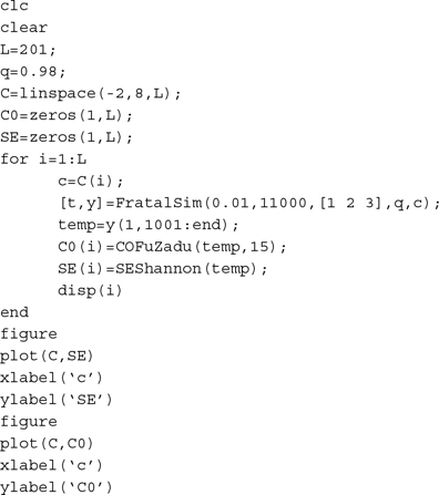
Running the above codes, the complexity of the fractional-order simplified Lorenz system with c varying can be obtained as shown in Figure B.8.

Figure B.8: Complexity of the fractional-order simplified Lorenz system with c varying (q= 0.98): (a) SE complexity and (b) C0complexity.
5.Program for complexity-based chaos diagram:


Figure B.9: Chaos diagram of the fractional-order simplified Lorenz system on q–c plane: (a) based on SE complexity and (b) based on C0 complexity.
Running the above codes, the complexity-based chaos diagram on q–c plane of the fractional-order simplified Lorenz system can be obtained as shown in Figure B.9.
It is worth pointing out that the greater the value of L, the more the mesh of the parameters plane, and the more details can be reflected. But the code running time is relatively long, and it needs to wait patiently. We suggest to choose L = 101 at least. At the same time, the length of the sequence is also important when we calculate the complexity. Because both the SE algorithm and C0 algorithm are based on fast Fourier transformation, the length of the sequence is suggested to choose N = 104. For test, we choose L = 51 and N = 104.
B.4Simulation of Chaotic Synchronization
B.4.1Drive–Response Synchronization


It will be very convenient to solve this problem by using the Matlab Ode45 function, if the drive system and the response system are considered as a big system. Of course, readers can also solve the drive system and input the drive system sequence into the response system, but the program may be relatively complex:
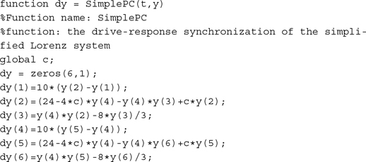
Setting c = –1, initial values of the drive system are [5, 8, –10] and the initial values of the response system are [5, –5, 20]. Running the below Matlab codes, the synchronization error curves of the synchronization system are obtained as shown in Figure B.10:


Figure B.10: Synchronization error curves of the simplified Lorenz system: (a) error curve of sequence x; (b) error curve of sequence y; and (c) error curve of sequence z.
B.4.2Coupling Synchronization


Figure B.11: Coupling synchronization error curves of the simplified Lorenz system: (a) error curve of sequence x; (b) error curve of sequence y; and (c) error curve of sequence z.
Setting c = 2, k1 = 4, k2 = 2, and k3 = 3, the initial values of the drive system are [4, 5, 6] and the initial values of the coupling system are [1, 2, 3]. Running the Matlab codes below, the synchronization error curves of the synchronization system are obtained as shown in Figure B.11:

B.4.3Tracking Synchronization

Design the controller:
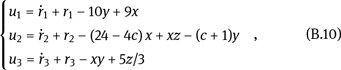
where r1, r2, and r3 are signals to be tracked.
Next, we let the simplified Lorenz system to track the sin curve, the constant curve, and the x sequence of the hyperchaotic Lorenz system, respectively,


Figure B.12: Tracking curves of the simplified Lorenz system: (a) sequence x; (b) sequence y; and (c) sequence z.
Running the above Matlab codes, the tracking curves of the simplified Lorenz system are obtained as shown in Figure B.12. Of course, readers can also plot the tracking error curves.