
8Analysis and Simulation of Fractional-Order Chaotic System
With the further research of nonlinear chaotic theory, fractional-order chaotic system has become a hot topic. To apply the fractional-order chaotic system in the field of information security, it is necessary to reveal its characteristics. Moreover, key technical problems are required to be solved quickly, such as accurate solution of fractional differential equations, digital signal processing (DSP) circuit realization, and so on. In this chapter, we focus on solution algorithm and simulation technology. It is the theoretical and experimental basis for applications of fractional-order chaotic system.
8.1Development of Fractional-Order Chaotic System
Theoretical research of fractional calculus has more than 300 years history, and it has the same long history as the integer-order calculus. However, due to the lack of application background, its development is relatively slow. Actually, fractional dynamic behavior can be observed in many physical systems, such as viscous system, dielectric polarization, colored noise, electromagnetic waves, and so on. Compared to integer-order calculus equation, fractional-order equation can describe nature phenomenon more accurately in applied science areas [161] such as memory of various materials, mechanics and electrical characterization, viscoelastic dampers, power fractal network, fractional-order sinusoidal oscillator, robots, electronic circuits, electrolytic chemical, fractional capacitance theory, fractal theory, fractional proportional– integral–derivative controller, viscoelastic vibration control system, flexible configuration object, and so on. Since Mandelbort first reported that there are numerous fractal phenomena in nature in 1983 [162], fractional calculus has become a hot topic and has developed quickly.
At the beginning, the investigation of fractional-order chaotic system was based on the research of integer-order chaotic system. When fractional differential operator is introduced to nonlinear dynamic system, the fractional-order system still exhibits chaotic behavior, such as Chua circuit [163], a nonautonomous Duffing system [164], improved Duffing system [165], fractional Jerk system [166], Rössler system [167], and so on. Although dynamic characteristics of some fractional-order chaotic system have been investigated, there still remain many other fractional-order chaotic systems to be studied.
Up to now, there are many definitions about fractional-order calculus [168]. Li and Deng studied three definitions of fractional-order calculus deeply [169]. Among these definitions, Riemann–Liouville (R-L) definition and Caputo definition are usually used in practice. Although the R-L definition can simplify the calculations of fractional differential, its physical meaning is not clear and its value is difficult to be measured. However, when using Caputo definition, its physical meaning of fractional differential is clear and its value is easy to be measured. Based on these two definitions, people proposed two different approximate methods for solving the fractional differential equation. One is time–frequency method based on R-L definition [170]. First, the fractional integral operator in the time domain is transformed into transfer function in frequency domain. Then piecewise linear approximation method is used to realize approximation calculation in frequency domain. The other is predictor– corrector method based on Caputo definition [171–173]. It is a time domain method. The time series of the fractional-order system are obtained by Adams–Bashforth prediction equation and Adams–Moulton correction equation. However, frequency domain method cannot reflect the dynamic characteristic of fractional-order chaotic system accurately. As for the time domain method, the calculation step can be set small enough for more accuracy, but its calculation is more complex relatively.
By far, the chaotic characteristic study of fractional-order system is mainly based on existing integer-order chaotic system. The main idea is to observe whether the systemis still chaotic when the system order changed from integer to fractional. However, the system order when system entering into chaotic still needs further research, as well as dynamic characteristic of fractional-order chaotic system. For example, Ahmad reported that when the order of system is 2 + ε (0 < ε < 1), third-order chaotic systems still perform chaotic behavior [6]. And fourth-order chaotic systems still perform hyperchaotic behavior when the system order is 3 + ε (0 < ε < 1) [174]. Obviously, the range of ε is too big in this case. Is it possible to narrow? For example, fractional-order Chua system performs chaotic behavior when the order is 2.7. People get the conclusion only through observing system behavior when the system order is 2.7 and 2.6. So is it chaotic when the order is 2.65? As a result, smaller step size should be chosen and smaller error fractional differential approximation algorithm model should be designed. Besides, dynamic characteristics such as Lyapunov exponent spectrum, bifurcation, and dimension remain further research.
Synchronization technology is the key of application of chaotic system to secure communication. In 1990, Pecora and Corroll first proposed the concept of chaotic synchronization [10]. They also realized synchronization of two mutually coupled chaotic systems in the laboratory by using the same signal circuits driven [11]. In the next 20 years, chaotic synchronization developed a lot. Even though synchronization of integral chaotic system has achieved much research results, research of fractional-order system synchronization is still in the beginning because it is too complex and the effective mathematical tool is deficient. If we apply integral-order control method to fractional-order system, true characteristic will be ignored. As a result, studying control method of fractional-order chaotic system has practical significance.
By far, more effective synchronization control method has not been proposed for fractional-order chaotic system. In most cases, we develop integral chaotic synchronization method to fractional-order chaotic, so its synchronization control mechanism and performance need further study. Studies show that the mutual coupling synchronization, projective synchronization, and adaptive method have unique advantages on improve synchronization performance. The target of fractional-order system synchronization research is to improve system performance and finding general law when changing order and parameter. The most suitable synchronization method should be chosen through comparing synchronization establishment time and synchronization accuracy. It is significantly important to lay technical foundation for the application of fractional-order chaotic system in secure communication.
Application of fractional-order chaotic systems is becoming a new direction of nonlinear applied science research area [175], especially in the aspects of information secure communication. Complexity of fractional-order chaotic sequence is a key point of the system safety performance. It is directly related to the performance of cryptography of fractional-order chaotic encryption system. For example, to ensure maximum communication capacity of spread spectrum communication, practical chaotic pseudorandom code sequence should have the biggest complexity. Complexity of fractional-order chaotic system contains two meanings. One is for chaotic system, which is always related to nonlinear term of system equation. As for fractional-order system, it may also be associated with order. This kind of complexity is mainly measured by calculating system fractal. The other meaning is for complexity of time series generated by fractional-order chaotic system. It is mainly used to measure the similarity degree of time signal and random signal. Some parameters, for example, information entropy, Lyapunov exponent, and fractal dimension, are adopted to measure the degree of system disorder. But these methods are not suitable to describe the complexity of time sequence generated by chaotic system. Therefore, the phase space observation method and structural complexity algorithm should be combined to analyze the fractional-order chaotic system and corresponding chaotic pseudorandom sequence. It will provide basis for the application of fractional-order chaotic system to cryptography and secure communication.
Circuit implementation of fractional-order chaotic system is another key issue of chaotic secure communication. In 2006, Bohannan et al. [176] applied for a patent to design fractional devices. Liu led his team to achieve circuit simulation for a number of fractional-order chaotic system through designing equivalent circuit of fractional integral [177–179]. But these methods are all based on frequency domain method. Even though the time domain method has significant advantages in studying fractional-order chaotic system, its circuit implementation is quite difficult. However, as the development of microelectronics, it is possible to realize time domain approximate method based on Field Programmable Gate Array (FPGA) or DSP. This method is a new way to realize the application of fractional-order chaotic system.
In all, research of fractional-order chaotic system is still at the initial stage. There still remain a lot of theoretical and practical issues that need further study. In this chapter, we will analyze the relationship of dynamic characteristics and fractional order. Synchronization of fractional-order chaotic system will also be studied.
8.2Definition and Physical Meaning of Fractional Calculus
Generally, fractional calculus is denoted by the operator ![]() which indicates both of the fractional differential and the fractional integration. When q is positive, the operator represents fractional differential. When q is negative, it indicates fractional integration. Here, we introduce several common definitions about fractional calculus.
which indicates both of the fractional differential and the fractional integration. When q is positive, the operator represents fractional differential. When q is negative, it indicates fractional integration. Here, we introduce several common definitions about fractional calculus.
Definition 8.1: Gamma function Γ(x) is a basic function for fractional calculus, and its definition is
When x = n, Γ(n) = (n–1)!
Definition 8.2: Grünwald–Letnikov fractional calculus is defined as
Definition 8.3: Riemann–Liouville fractional calculus is defined as

where q ∈ R, n is the first integer greater than q, which means n – 1 ≤ q < n, Γ(⋅) is Gamma function. According to the above definition, q-order differential of power function and constant is
The Laplace transform of R-L fractional calculus is defined as
As the Laplace transform needs the value of noninteger-order differential at t = 0, it is difficult to solve Laplace transform of R-L fractional-order differential. However, it can be solved according to the Caputo definition of fractional differential
Definition 8.4: Caputo fractional differential is defined as

where m is the first integer greater than q. The Laplace transform of Caputo fractional differential is
When compared with Laplace transform of R-L fractional differential, for Caputo fractional differential, only integer-order differential is needed in Laplace transform. When the initial value of operator is zero, its corresponding Laplace transform is
Two basic properties of Caputo fractional differential definition are
Thus, the q-order differential of the power function and constant are defined as
Integer-order calculus has clear geometric interpretation and physical meaning. However, because of the complexity of fractional calculus, it is difficult to understand the concept of fractional calculus. Therefore, there exist some obstacles in practical applications. At present, fractional calculus does not have universal and unified physical meaning and geometric interpretation yet [180].
It is easy to get the physical meaning of fractional integral according to its definition. If we suppose integral as storage, then the fractional integral can be taken as memory storage. The fractional integral only store near information and abandon the past information gradually. Professor Liu et al. in Peking University described the fractional differential as a “bridge between weather and climate,” which means the fractional differential of climate is weather. It is the fractional differential that makes climate has greater memory than weather [181].
We can get some conclusions according to the definition of fractional differential. (1) The initial value of input function is added to the output as attenuate form. (2) When the initial value is zero, the fractional differential is formed as convolution. Thus, the fractional differential is actually an integral and it forgets characteristic gradually (or time decay of memory). (3) Introduction of the definition of R-L fractional differential can simplify the calculation of fractional derivative. (4) Introduction of the definition of Caputo fractional differential makes Laplace transform more concise, which benefits the calculation of fractional differential equation [182].
8.3Solution Methods of Fractional-Order Chaotic System
8.3.1Frequency Domain Method for Solving Fractional-Order Chaotic System
There are several methods and algorithms for solving fractional differential equations and fractional-order systems, for example, Laplace transform, Fourier transform algorithm, and numerical algorithms. However, these methods have some drawbacks. At present, people are most interested in using integer-order model to approximate the fractional-order system.
Bode graphics approximating method of the fractional-order system is realized by the time–frequency conversion. The transfer functions are calculated by piecewise linear approximation in frequency domain. This method is in favor of the project implementation. The idea is to obtain frequency domain expansion of fractional integral operator by solving 1/sα in frequency domain. And then the frequency domain function is transformed to the integer-order state equation [170]. This approximation error is within the permissible range and can fully meet the needs of engineering.
If the initial condition is set to zero, then the Laplace transform of R-L in formula (8.7) becomes to
Therefore, the fractional integral operator in frequency domain with q-order can be described by the transfer function F (s) = 1/sq. To analyze dynamics of fractional-order chaotic system effectively, standard integral-order operator is required to approximate fractional-order operators (Bode plot approximation). In this case, approximation error will definitely be within the permissible range and can fully meet engineering requirement. Fractional integral operators are defined as
where s = jω is complex frequency, and α is a positive fraction which is also called fractional power. Since the magnitude of this function is relatively big at low frequency and the system is of multifrequency, a fractional-order system with multifrequency can be described as

where 1/pTi is relaxation time and αi is fractional power factor. Formula (8.16) is called single structural model of single fractional-order system. Through a fractional extreme representation of single frequency, the transfer function in frequency domain can be represented as
where 1/pT is relaxation time and α is fractional power factor (0 < α < 1).
By using –20 dB segments with “zigzag” type to approximate, formula (8.18) can be approximated as [170]

where N represents the number of poles. Since working frequency in engineering practice is limited, the number of the above formula can be limited to N. Then the above formula can be further approximated as

As a result, the problem of getting the fractional function expression is transformed into the problem of finding zero-pole pair. If the approximation error is controlled within y dB (y is positive), the pole-zero pair is determined as follows:
The first pole: p0 = pT10y/(20α)
The first zero: z0 = p010y/(10(1–α)).
The second pole: p1 = z010y/(10α).
The second zero: z1 = p110y/(10(1–α)).
The Nth zero: zN+1 = pN+110y/(10(1–α)).
The (N+ 1)th pole: pN = zN+110y/(10(α)).
Here PT is the angular frequency and p0 is the first singular value which is determined by the setting error y. PN is the last singular value which is determined by N.
Now, let a = 10y/(10(1–α)), b = 10y/(10α), then we have
So the distribution relationship of zeros and poles can be written as
According to the above relationship and p0, we can obtain all zero-pole values:
N of formula (8.19) is deduced by the following procedure. The constraint relationship of system frequency bandwidth is
Therefore,


Generally, we set y = 2 dB or y = 3 dB, ωmax = 0.01–100 rad/s. According to the above formula, 1/sα in frequency domain is obtained. The expansion form of 1/sα is shown in Table 8.1 [166], where α changes from 0.1 to 0.9 and approximation error is 2 dB. When the approximation error is 3 dB, the expansion form of 1/sα is shown in Table 8.2 [163].
Table 8.1: α-Order fractional integral linearity conversion function approximation. (Approximation error is 2 dB.)

Table 8.2: α-Order fractional integral linearity conversion function approximation. (Approximation error is 3 dB.)

8.3.2Time Domain Method for Solving Fractional-Order Chaotic System
8.3.2.1Adams–Bashforth–Moulton Predictor–Corrector Scheme
A typical fractional-order time domain approximation method is Adams–Bashforth–Moulton predictor–corrector scheme [171–173]. This method is described as follows.
For the differential equation
It equals Volterra integral equation

Obviously, the two parts of the right side in the above equation totally determined by the initial value. A typical case is 0 < q < 1, and the Volterra equation has weak singularity. In Refs [171–173], a predictor–corrector scheme for eq. (8.35) is reported. It can be regarded as a similar algorithm of Adams–Moulton algorithm with one step.
Let h = T/N, tj = jh (j = 0, 1, 2, . . . ,N), where T is the integral upper limit of this equation. Then the corrector formula of eq. (8.35) is given by
where
Then we use one-step Adams–Bashforth rule to replace one-step Adams–Moulton rule. The predictor term ![]() is given by
is given by
where
The basic algorithm of fractional-order Adams–Bashforth–Moulton method is shown in formulas (8.36) and (8.38), where aj,n+1 and bj,n+1 are presented in formulas (8.37) and (8.39), respectively. The estimate error of this method is ![]() o(hp), where p = min (2,1+ q). Although the time domain method is more complex than the frequency domain method, the step size can be smaller, and it is much better for analysis of dynamics of fractional-order system.
o(hp), where p = min (2,1+ q). Although the time domain method is more complex than the frequency domain method, the step size can be smaller, and it is much better for analysis of dynamics of fractional-order system.
8.3.2.2Adomian Decomposition Algorithm
Adomian decomposition algorithm (Adomian decomposition method, ADM) is a time domain approximation method for solving fractional-order system [183]. This method is used to solve linear and nonlinear problems. The corresponding approximate numerical solution is highly accurate with fast convergence. Moreover, it needn’t be discreted and too many computer memories. The numerical solutions of fractional-order Chen system and fractional-order Rössler system based on ADM are studied [184, 185], which proves the effectiveness of the algorithm.
If the fractional-order chaotic system is ![]() where x(t) = [x1(t), x2(t), . . . , xn(t)]T is the functional variable and g(t) = [g1(t), g2(t), . . . , gn(t)]T is the constant term for autonomous system and f includes both linear and nonlinear terms, then the system can be separated into three parts by
where x(t) = [x1(t), x2(t), . . . , xn(t)]T is the functional variable and g(t) = [g1(t), g2(t), . . . , gn(t)]T is the constant term for autonomous system and f includes both linear and nonlinear terms, then the system can be separated into three parts by

where ![]() represents q-order Caputo differential operator. L represents the linear term. N represents the nonlinear term, and bk is the initial value. Applying the integral operator to both sides of the equation, we have
represents q-order Caputo differential operator. L represents the linear term. N represents the nonlinear term, and bk is the initial value. Applying the integral operator to both sides of the equation, we have
where ![]() is the initial value. According to the Adomian decomposition algorithm, the solution of the equation can be represented as
is the initial value. According to the Adomian decomposition algorithm, the solution of the equation can be represented as ![]() The nonlinear term can be decomposed as
The nonlinear term can be decomposed as

where i = 0,1, . . . , and j = 1,2, . . . , n. The nonlinear term is
Then, the solution of the equation is
where its iterative relationship is

Next, we take fractional-order simplified Lorenz system as an example to explain this method further.
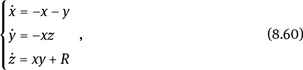
The differential equations of fractional-order simplified Lorenz system with a parameter c is [186]

The linear and nonlinear terms of system are decomposed as

According to eq. (8.44), the first seven items of nonlinear term are [187]


According to the given initial values, we have

Let ![]() which means
which means ![]() According to
According to ![]()
![]() in formula (8.45) and properties of fractional calculus, we have
in formula (8.45) and properties of fractional calculus, we have

If ![]() then x1 = c1(t – t0)q/Γ(q + 1). So we only need to solve the corresponding coefficient of eachterm. According to formula (8.46), the other five coefficients are obtained as
then x1 = c1(t – t0)q/Γ(q + 1). So we only need to solve the corresponding coefficient of eachterm. According to formula (8.46), the other five coefficients are obtained as


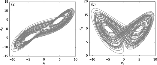
Figure 8.1: Attractor of fractional-order simplified Lorenz system: (a) x1–x2 plane and (b) x1–x3 plane.
So the solution of system equation is

where j = 1, 2, 3. Then we can get the analytic solution of system variable. In practical calculation, the time period [t0, t] should be divided into smaller time interval [tk, tk+1]. In each interval, t0 is set as tk, and then the value of corresponding tk+1 is obtained. The attractor phase diagram of fractional-order simplified Lorenz system based on formula (8.57) is shown in Figure 8.1. In this figure, the length of small time interval is 0.01 s. The initial values are [0.1, 0.2, 0.3]. Parameter c = 5 and fractional order q = 0.98.
8.4Simulation Method for Fractional-Order Chaotic System
8.4.1Dynamic Simulation Method for Fractional-Order Chaotic System
Dynamic simulation analysis method is to use the dynamic model to represent the state change over time, and the dynamical characteristics of the system are analyzed by observing the real-time evolution of the variables. By employing this method, we can directly observe the simulation results and also can make a quantitative analysis for the simulation output data. It has the characteristics of intuition and flexibility. Based on frequency domain analysis method of fractional calculus operator, fractional-order system simulation model is designed through state-space module in Simulink. State-space module is a state-space description module for input–output variables, which is defined as
where x is the state vector, u is the input vector, and y is the output vector. A, B, C, and D are coefficient matrices. Obviously, those modules receive inputs and then generate outputs. Parameters of coefficient matrices A, B, C, and D are corresponding to that of transform function, respectively, which can be calculated by tf2ss transform function in Matlab.
Steps of the dynamic simulation are as follows:
- Determine the function modules listed according to the differential equation of fractional-order chaotic system. The simulation system is built by connecting these modules.
- Set simulation parameters. It includes system operating parameters (e.g., system operating time, integration step size, tolerance error, integration algorithms, etc.) and function modules operating parameters (such as integrator initial value, signal amplitude, frequency, etc.).
- Set observation module. It is used to output data and observe operation status of simulation system.
- Analyze the simulation results. Simulation results are analyzed by output data and waveform, and compared with that of theoretical analysis. If it is not consistent with each other, the model and parameters should be revised.
During the simulation, Scope module is used to show real-time output signal dynamically. Phase diagram can be observed by XY graphmodule. In phase space, convergence motion corresponds to the equilibrium point, periodic motion corresponds to a closed trajectory, and chaotic motion corresponds to random separation of the never closed trajectory in a certain region (strange attractor). So, the output phase diagram of XY graphmodule is used to preliminarily judge whether the system is chaotic. Out module can save results to workspace automatically, so the saved data can be output by yout() function, and it is used to calculate the power spectrum and the maximum Lyapunov exponent of the system.
How to set the state-space module is the key of realizing dynamic simulation of fractional-order chaotic system. Parameter matrices A, B, C, and D in the property dialog box are determined by the order of fractional-order system. To obtain each matrix element, we can call command [A,B,C,D] = TF2SS(NUM,DEN) (where NUM represents the molecular coefficient matrix and DEN represents the denominator coefficient matrix) or [A,B,C,D] = ZP2SS(Z,P,K) (where Z represents the zeros matrix of transform function, P represents the poles matrix, and K represents the coefficient).
For example, when q = 0.95, the transform function of fractional-order integral operator is written as [167]
For formula (8.59), calling format of the function TF2SS is [A,B,C,D] = TF2SS (1.2831,18.6004,2.0833], [1,18.4738,2.6547,0.003]). Its corresponding return value is

Next, we take the fractional-order diffusionless Lorenz system as an example to explain further. The diffusionless Lorenz system is
where R is the parameter of system. When R ∈ (0, 5), the system is chaotic. Its corresponding fractional-order diffusionless Lorenz system is written as

where 0 < α, β, γ ≤ 1 are fractional orders. Dynamic simulation model of the system is constructed as shown in Figure 8.2. The initial values of system are set as [0.3782, 0.6748, 2.8831]. Let α = β = γ = 0.95 and simulation time is 200 s. By using ODE45 differential equation solvers, the strange attractor of diffusionless Lorenz system in x–z plane is shown in Figure 8.3.
8.4.2Circuit Simulation Method of Fractional-Order Chaotic System
Design of fractional integral operator circuit is the key of Electronics Workbench circuit simulation for fractional-order chaotic system. Because the fractional integral operator with q-order is described by transform function F (s) = 1/sq in frequency domain, the unit circuit as shown in Figure 8.4 is used to achieve the expansion of 1/sq [177]. The nonlinear terms are realized by multipliers. Then the equivalent circuit of the fractional-order system is constructed.
In Figure 8.4, system function of the equivalent circuit between A and B is described as

Figure 8.2: Simulation model of the fractional-order diffusionless Lorenz system.


where n is the highest order of s in denominator of 1/sα when q varied from 0.1 to 0.9. For example, when q = 0.95, n = 3, according to eq. (8.59), we have
Comparing eq. (8.63) with eq. (8.59), we have R1 = 15.1 kΩ, R2 = 1.51 kΩ, R3 = 692.9 MΩ, C1 = 3.616 μF, C2 = 4.602 μF, C3 = 1.267 μF. Resistors and capacitors of 1/sq calculated in Ref. [166] are shown in Tables 8.3 and 8.4, respectively [177].
The circuit of fractional-order diffusionless Lorenz system is shown in Figure 8.5, in which the resistance values are R1 = R2 = R3 = R4 = R7 = 10 kΩ, R6 = R8 = R9 = 100 kΩ, R5 = R10 = 1 MΩ. “Fraction” is the integrator unit circuit of 0.95-order after packaged. When R =5 and q = 2.85, its attractor of x–z plane is shown in Figure 8.6. Obviously, it is consistent with that of simulation result as shown in Figure 8.3.
Table 8.3: Resistance of fractional-order integrator unit circuit with order α.

Table 8.4: Resistance of fractional-order integrator unit circuit with order α.


Figure 8.5: Circuit simulation model of diffusionless Lorenz system with q = 0.95.

8.4.3Numerical Simulation Method of Fractional-Order Chaotic System
Numerical simulation method is to transform the mathematic model of fractional-order chaotic system into recursive calculation form which is suitable for processing on a computer. The main advantage of this method is that it can solve complex problems analytically. The basic steps are as follows [188]:
- Establish mathematical model for fractional-order chaotic system.
- According to the characteristic of this model, choose suitable software as simulation tool and design the computer program according to the mathematical model.
- Run the program and get the numerical solution of the system.
- According to the numerical solution, analyze dynamic characteristic such as calculating Lyapunov exponent and fractal dimension.
For example, according to the approximation formula based on Adams–Bashforth–Moulton time domain method, the fractional-order diffusionless Lorenz chaotic system is presented as

where


Based on Matlab, we let α = β = γ = 0.95, R = 5, h = 0.01, T = 200, and the computer program is designed. The chaotic attractor of fractional-order diffusionless Lorenzchaotic system with q = 0.95 is shown in Figure 8.7. Obviously, it is consistent with the results of dynamic simulation and circuit simulation.

Figure 8.7: Attractor of fractional-order diffusionless Lorenz system based on numerical simulation.
8.4.4Comparison of Simulation Methods
1.Comparison among dynamic simulation, circuit simulation, and numerical simulation based on predictor–corrector method. The three simulation methods have their own advantages and disadvantages. We summarized their features as shown in Table 8.5 from the aspects of analysis method, fractional order change, result output, and simulation speed. Dynamic simulation method can construct dynamic system model quickly by employing abundant functional blocks in Simulink. You don’t need to write a line of codes. When simulating complicated fractional-order nonlinear chaotic system, this method is more simple and intuitive. However, its limitation is that the value of q can only take finite value. Circuit simulation has similar characteristic with dynamic simulation, but because the circuit simulation is more close to the realistic engineering system, it is more important for the application of the fractional-order chaotic system. Programming is required for numerical simulation, and dynamic output process of variable evolution cannot be observed directly. But when the value of fractional-order changes continuously, it is more convenient to analyze the chaotic characteristic of the fractional-order system.
Table 8.5: Comparison of simulation methods.

Table 8.6: Comparison between numerical simulation methods for fractional-order chaotic system.
| Adomian method | Predictor–corrector scheme | |
| Time complexity | O(n), fast | O(n2), slow |
| Space complexity | O(1), small | O(n), large |
| N = 1, 000 | 0.9701 s | 2.0154 s |
| N = 2, 000 | 1.8403 s | 7.7051 s |
| N = 5, 000 | 4.5162 s | 51.3995 s |
2.Comparison between ADM and predictor–corrector scheme. Both of them are time domain methods. Comparison of time complexity and space complexity of the two methods is shown in Table 8.6. It can be seen that the ADM is better than predictor–corrector method from both of these two aspects. The data in last three lines of Table 8.6 is the requirement time for getting time series with the different lengths (the results are different with different CPU frequencies. Here, the computer parameter is Intel Dual E2180 2.0 GHz). It can be seen that the growth rate of time required for predictor–corrector method is much faster than that of Adomian decomposition algorithm. So, we can get the conclusion that Adomian decomposition algorithm is better than predictor–corrector scheme when solving fractional-order chaotic system.
In this section, we analyzed three simulation methods of fractional-order chaotic system. For different methods, design methods and simulation steps are described. Furthermore, to show the effectiveness of different simulation methods, the fractional-order diffusionless Lorenz chaotic system is simulated based on Matlab, Simulink, and EWB.
8.5Dynamics of Fractional-Order Unified System Based on Frequency Domain Method
In this section, we use dynamic simulation method to analyze fractional-order unified system based on Matlab/Simulink.
8.5.1Fractional-Order Unified Chaotic System Mode
In 2002, a new chaotic system is proposed [84], which connects Lorenz attractor and Chen attractor. Meanwhile, Lü system is a special case of this system. So it is called unified chaotic system [189], and its mathematic model is

where a is the system parameter. When a ∈ [0,1], it is chaotic. This system represents a family of chaotic system. Chaotic attractor in x–z plane of unified chaotic system with different parameters is shown in Figure 3.20.
After replacement of integer-order differential operator with fractional-order differential operator, fractional-order unified system becomes

where α, β, and γ are fractional orders and system parameter a ∈ [0,1]. The fractional order for different variables x, y, and z may be different. The principle is the same for different fractional orders or the same fractional order. Here, we set 0 < α = β = γ = q ≤ 1 to analyze fractional-order unified system.
8.5.2Dynamic Simulation of Fractional-Order Unified Chaotic System
In this section, we focus on the dynamics of the fractional-order unified chaotic system by Simulink simulation
8.5.2.1Simulation Model
When a = 1, eq. (8.69) becomes

According to eq. (8.70), when we design the model of fractional-order system, some modules are required, including state-space module, gain module, sum module, and produce module. Based on Simulink, we copy the required modules from module library to edit window, and then connecting these modules according to system (8.70) as shown in Figure 8.8.
8.5.2.2Setting Simulation Parameter
After the model is set up simulation environment and parameters are required to be configured. By choosing menu “Simulation: Simulation Parameters” in the model window, the simulation configuration dialog will pop up. Then we modify simulation configuration. Almost all of the modules have dialog box for property setting. By double-clicking the module or clicking “Edit: BLOCK Propertied” after choosing the module, a basic properties dialog box will be opened. In this dialog, users can set the basic properties of the module.

Figure 8.8: Simulation model of fractional-order unified system with a = 1.
In state-space module, the values of parameters A, B, C, and D are determined by the value of fractional order as explained in Section 8.4.1. The initial values of system are set by the initial condition. The other parameters are set as default values. Here, the initial values are set as (0.1, 0.1, 0.1) and simulation time is set as 30 s. The ODE45 differential equation solver is used to solve the equation.
8.5.3Dynamics of Fractional-Order Unified System with Fixed Parameter
According to eq. (8.70), we analyze dynamics of the fractional-order unified system with q = 0.1–1, changing parameter or order.
8.5.3.1Direct Observation Analysis
According to direct observation method, period motion in the phase space corresponds to a closed curve, while chaotic behavior corresponds to a never closed trajectory which is random separated in a certain area (strange attractor). After we finish the simulation of fractional-order chaotic system, the time sequence diagram and system phase diagram are plotted. Then we can preliminarily determine whether the fractional-order system is chaotic.
According to the fractional-order unified system model, the Scope module and XYgraph module are used to observe simulation results.

Figure 8.9: Attractors in the x–z plane of fractional-order unified system with different orders: (a) q=0.1, (b) q = 0.2, (c) q = 0.3, (d) q = 0.4, (e) q = 0.5, (f) q = 0.6, (g) q = 0.7, (h) q = 0.8, and (i) q = 0.9.
Let q = 0.1–1 and set step size as 0.1. Simulation time is set to 40 s. For different fractional orders, we get the trajectory in x–z phase plane as shown in Figure 8.9. It can be seen that there exist the random separate states in the phase space when q = 0.1–0.3 and q = 0.8–1. It means chaotic attractor exists and the system is chaotic in this case. When q = 0.4–0.7, the phase curve finally converges to one point, which means the system is in periodic state.
By observing phase diagrams of the fractional-order unified system directly, we get the following conclusions. When q = 0.1–0.3, the system is chaotic. When q = 0.4–0.7, the system is periodic. When q = 0.8–1, the system shows chaotic behavior again. Therefore, fractional-order unified system is piecewise chaotic.
8.5.3.2Power Spectrum Analysis
In this section, we will use power spectrum analysis method mentioned in Section 2.2 to analyze the fractional-order unified system. Power spectrum analysis can provide frequency information of signals. Discrete power spectrum corresponds to periodic behavior, while continuous power spectrum corresponds to chaotic behavior. So we can tell whether the system is chaotic or not by observing power spectrum. Based on Matlab, we calculated normalized power spectrum when fractional order q = 0.1–1, which is shown in Figure 8.10.

Figure 8.10: Normalized power spectrum density of fractional-order unified system with different orders: (a) q = 0.1, (b) q = 0.2, (c)q = 0.3, (d) q = 0.4, (e) q = 0.5, (f) q = 0.6, (g) q = 0.7, (h) q = 0.8, and (i) q = 0.9.
From Figure 8.10, we get the following conclusions. When q=0.8–1 and q = 0.1–0.3, the power spectrum is continuous, which means the system is chaotic. When q = 0.4–0.7, the power spectrum is discrete, which means the system is periodic. Therefore, by observing power spectrum, the fractional-order unified system is piecewise chaotic, which is consistent with the conclusion obtained by direct observation.
8.5.3.3Analysis of the Largest Lyapunov Exponent
Lyapunov exponent represents the average ratio of convergence or divergence of the system variables in the phase space. It is an important parameter to determine whether the system is chaotic or not. If the largest Lyapunov exponent is greater than zero, the system is chaotic definitely.
Table 8.7: Largest Lyapunov exponent of unified system with different order q.
| q | System order | The largest LE |
| 0.1 | 0.3 | 0.2180 |
| 0.2 | 0.6 | 0.1616 |
| 0.3 | 0.9 | 0.1249 |
| 0.4 | 1.2 | –0.0050 |
| 0.5 | 1.5 | –1.4618 |
| 0.6 | 1.8 | –0.0032 |
| 0.7 | 2.1 | –0.0078 |
| 0.8 | 2.4 | 0.0199 |
| 0.9 | 2.7 | 0.0756 |
| 1 | 3 | 0.0263 |
Here, we use Wolf method [190] to calculate the largest Lyapunov exponent of fractional-order unified system. When the fractional order q = 0.1–1 with step size of 0.1, the results are shown in Table 8.7. When q = 0.8–1 and q = 0.1–0.3, the largest Lyapunov exponent is positive, which means the system is chaotic. When q = 0.4–0.7, the largest Lyapunov exponent is zero, which means the system is periodic. Thus, from the largest Lyapunov exponent, we can get the conclusion that the system is piecewise chaotic [191].
8.5.4Dynamics of Fractional-Order Unified System with Different Parameter
8.5.4.1Dynamics with Different Parameter and Order
We analyzed chaotic characteristic of fractional-order unified system with fixed parameter (a= 1). Next, we use the above methods to analyze dynamics of fractional-order unified system when parameter a = 0–1 and step size is 0.1. The variation of fractional order is still between 0.1 and 1 and its step size is 0.1. Dynamics of fractional-order unified system with different parameters is shown in Table 8.8. However, when q = 1, the system is integer-order unified system. When parameter varies from 0 to 1, the system is always chaotic. From Table 8.8, we can get the following conclusion. When a = 0, system changes from chaotic to nonchaotic with the increase of order q. More specifically, system is chaotic at q = 1 and nonchaotic at the range of 0 < q ≤ 0.9. When a = 0.1–0.3, the system is chaotic at q = 1 and q = 0.1. It is nonchaotic at the range of 0.2 ≤ q ≤ 0.9. When a = 0.4–0.7, the system is chaotic at q = 1 and at the range of 0.1 ≤ q ≤ 0.3. It is nonchaotic at the range of 0.4 ≤ q ≤ 0.9. When a = 0.8–1, the system is chaotic at the range of 0.8 ≤ q < 1 and 0.1 ≤ q ≤ 0.3, and it is nonchaotic at the range of 0.4 ≤ q ≤ 0.7.
Obviously, dynamics of fractional-order unified chaotic system is related to both the system parameter and the fractional order. When the system parameter is fixed, the system is piecewise chaotic. When the fractional order is fixed, it is possible for the system to change from nonchaotic to chaotic. Besides, it can be seen that with the increase of parameter and order, the chaotic range of the system expands, while the nonchaotic range of order narrows.
Table 8.8: Status of fractional-order unified system with different parameter.

8.5.4.2Routes to Chaos with Fixed Fractional Order and Parameter Varying
We take q = 0.3 as an example to discuss the routes to chaos of the fractional-order system. When the initial values are (–4.7508, –7.3886, 12.3605) and parameter a = 0–1, the phase diagram on the x–z plane of fractional-order unified system is shown in Figure 8.11. When the system parameter a is relatively small, the system converges to the equilibrium point (as shown in Figure 8.11(a), 8.11(b), and 8.11(c)). However, with the increase of a, the evolution time of state variable tending to the equilibrium point becomes longer (as shown in Figure 8.11(d) and 8.11(e)). As a further increase to a certain value, such as a = 0.49, system reaches a border of attraction basin. At this time, system enters into chaos through boundary crisis bifurcation (as shown in Figure 8.11(f)). However, if we pursue accurate analysis for routes to chaos of fractional-order system, complex mathematical analysis and calculation are required.

Figure 8.11: Attractors in the x–z phase of unified system with different parameter and q = 0.3: (a) a = 0, (b) a = 0.1, (c) a = 0.2, (d) a = 0.3, (e) a = 0.45, and (f) a = 0.49.
By observing system phase diagrams and calculating power spectrum and the largest Lyapunov exponent, we analyzed dynamical characteristic of fractional-order unified system in detail. We also find that system shows piecewise chaotic behavior with the variation of system parameter and differential order.
8.6Dynamics of Fractional-Order Diffusionless Lorenz System Based on Time Domain Method
8.6.1Fractional-Order Diffusionless Lorenz System Model
The mathematic model of diffusionless Lorenz system is

where R is the system parameter. When R ∈ (0, 5), there exist equilibrium points ![]() The eigenvalues of this system satisfy the equation λ3 + λ2 + Rλ + 2R = 0.When R = 3.4693, the chaotic attractor of diffusionless Lorenz system is shown in Figure 8.12(a). Its maximum Kaplan–Yorke fractal is 2.23542 [192].
The eigenvalues of this system satisfy the equation λ3 + λ2 + Rλ + 2R = 0.When R = 3.4693, the chaotic attractor of diffusionless Lorenz system is shown in Figure 8.12(a). Its maximum Kaplan–Yorke fractal is 2.23542 [192].

Figure 8.12: Attractors of diffusionless Lorenz system with R = 3.4693: (a) α = β = γ = 1 and (b) α = β = γ = 0.95.
Correspondingly, the fractional-order diffusionless Lorenz system is

where α, β, and γ are the fractional order and 0 < α, β, γ ≤ 1. When α = β = γ=0.95 and R = 3.4693, the chaotic attractor of diffusionless Lorenz system is shown in Figure 8.12(b).
According to the previous discussion about time domain solution algorithm of the fractional-order system, we can get the iterative calculation equation of fractional-order diffusionless system as shown in eq. (8.64). Next, we analyze its dynamic characteristic in detail.
8.6.2Chaotic Characteristic of Fractional-Order Diffusionless Lorenz System
Here, we adopt Wolf algorithm [190] calculating the largest Lyapunov exponent. Let α = β = γ = q and control the variation of parameter, we can get the effective chaotic range of frictional-order diffusionless system as shown in Figure 8.13. Obviously, there exist three different dynamic statuses: limit circle, chaos, and convergence. If the integer-order system is chaotic, the corresponding chaotic range of fractional-order system will narrow slowly with the increase of system control parameter. If the integer-order system shows limit circle, the corresponding fractional-order system is chaotic. But the chaotic range will narrow quickly with the increase of system parameter. When R = 8, the largest Lyapunov exponent of fractional-order diffusionless Lorenz system is shown in Figure 8.14. Obviously, its chaotic characteristic is consistent with the chaotic range as shown in Figure 8.13.

Figure 8.13: Chaos range of fractional-order diffusionless Lorenz system.

Figure 8.14: The largest Lyapunov exponent of fractional-order diffusionless Lorenz system with R = 8.
8.6.3Bifurcation Analysis with Varying System Parameter R
Here, we set the fractional order α = β = γ = 0.95 and let the system control parameter R vary from 0.5 to 11 with the step size of 0.01. The initial values are x(0) = –0.0249, y(0) = –0.1563, and z(0) = 0.9441, and the simulation time is 140 s. The bifurcation diagram of fractional-order system is shown in Figure 8.15. Obviously, when the order of fractional-order diffusionless system is 2.85 and R varies, the system is chaotic with a periodic window. When the control parameter R decreased from 11, the fractional-order diffusionless system enters into chaotic by period-doubling bifurcation as shown in Figure 8.16 (the step size is 0.005). In periodic window, several bifurcations are observed, such as an interior crisis bifurcation at R ≅ 5.57, a flip bifurcation at R ≅ 6.02, and a tangent bifurcation at R ≅ 6.55. In the interior crisis, the chaotic attractor collides with an unstable periodic orbit or limit cycle within its basin of attraction. When the collision occurs, the attractor suddenly expands in size but remains bounded. For the tangent bifurcation, a saddle point and a stable node coalesce and annihilate one another, producing an orbit that has periods of chaos interspersed with periods of regular oscillation [193]. This same behavior occurs in the periodic windows of the logistic map, including the small windows within the larger windows [194]. In this periodic window, we also observe the route to chaos by a period-doubling bifurcation.

Figure 8.15: Bifurcation diagram of fractional-order diffusionless system with R varying at q = 0.95.

8.6.4Bifurcation Analysis with Varying Fractional Order q
Now, we set α = β = γ = q, R = 8 and q varying from 0.9 to 1. The initial values and running time kept the same as above, but the step size of R is 0.0005. The system bifurcation diagram is shown in Figure 8.17. The system enters into chaos by period-doubling bifurcation with decreasing fractional order. It is interesting to note that a chaotic transient is observed when q is less than 0.912. The state-space trajectory is shown in Figure 8.18(a) for q = 0.911, which suddenly switches to a pattern of oscillation that decays to the right equilibrium point. The time domain waveform of variation z(t) shown in Figure 8.18(b) eventually converges to the fixed point. On the average, the transform from chaotic behavior into damped state requires about 70 oscillations. When q is relatively greater, its chaotic behavior will remain longer. Similar phenomenon has been reported in the standard Lorenz system [195]. The fractional-order system enters to chaos by a period-doubling bifurcation as shown in Figure 8.19(a) with steps in R of 0.0002. System is chaotic when q ∈ [0.92,0.962]. To observe dynamics in the periodic window, the periodic window is expanded as shown in Figure 8.19(b) with steps of 0.0001. Obviously, there exist three kinds of bifurcations, such as a tangent bifurcation, a flip bifurcation, and an interior crisis. The fractional order parameter can be taken as a bifurcation parameter, just like the control parameter.


Figure 8.18: Transient chaotic behavior in system (8.72) with R = 8 and q = 0.911: (a) attractor diagram in the x–y–z plane and (b) time domain waveform.
8.6.5Bifurcations with Different Fractional Order
1.Fix β = γ = 1, R = 8 and let α vary. The system is calculated numerically for α ∈ [0.4,1] with an increment of 0.002. The bifurcation diagram is shown in Figure 8.20(a). Obviously, the fractional-order system is chaotic when α ∈ [0.43,0.94) and it is periodic when α ∈ (0.484,0.503). The periodic window is expanded as shown in Figure 8.20(b) with steps of 0.0002. When α increases from 0.4, or decreases from 1, a period-doubling bifurcation route to chaos is observed.

Figure 8.19: Bifurcation diagram of fractional-order diffusionless Lorenz system at R = 8: (a) q ∈ [0.95, 1] and (b) q ∈ [0.93, 0.95].

Figure 8.20: Bifurcation diagrams of fractional-order diffusionless Lorenz system with α at β = γ = 1: (a) α ∈ [0.4, 1] and (b) α ∈ [0.48, 0.52].
2.Fix α = γ = 1, R = 8 and let β vary. The step of β is 0.001. The system is calculated numerically for β ∈ [0.75,1] with an increment of β equal to 0.001. The bifurcation diagram is shown in Figure 8.21. Obviously, when β decreased from 1, the fractional-order system enters into chaos by period-doubling bifurcation. When β is less than 0.8, the system converges to a fixed point. Thus, the minimum order of fractional-order diffusionless Lorenz system is 2.8 in this case.
3.Fix α = β = 1, R = 8 and let γ vary. The step of γ is 0.001. The system is calculated numerically for γ ∈ [0.8,1]. The bifurcation diagram is shown in Figure 8.22(a). It has similar dynamics with the previous two cases, which enters into chaotic by period-doubling bifurcation. Finally, the system converges to a fixed point at γ = 0.816. However, its range of chaotic order is smaller. The dynamic behaviors in the periodic window are similar with the case of (2) as shown in Figure 8.22(b) with steps of 0.0002.


Figure 8.22: Bifurcation diagrams of fractional-order diffusionless Lorenz system with γ at α = β = 1: (a) γ ∈ [0.8, 1] and (b) γ ∈ [0.81, 0.86].
The analysis results mentioned above show the fractional-order diffusionless Lorenz system has rich dynamical behaviors. It provides a theoretical and simulation basis for practical application of fractional-order chaotic system.
Questions
- What is the difference and relationship between fractional-order chaotic system and integer-order system?
- For fractional-order chaotic system, which solving method is the best?
- What are the methods of dynamic analysis for fractional-order chaotic system?
- Compare characteristics among different simulation methods for fractional-order chaotic system.
- Choose an integer-order chaotic system to analyze its corresponding fractional-order dynamic characteristic.