
In the previous chapters, we looked at data structures. At this point, you have more knowledge of data structures than a lot of people I have spoken to. While you may not know them inside out, you still have enough knowledge to at least know the purpose of each major data structure and may be able to apply them to solve your problems. In this chapter, we will deviate from looking solely at data structures and look at algorithms as well.
Mathematical Concepts
Prior to beginning our discussion on algorithms, there are a few mathematical concepts we must look at. These concepts will form the basis of understanding algorithms later when we discuss them.
Linearity
Before we get to any other discussions concerning algorithms, we can take a little time and talk about the concept of linearity. Figure 6-1 shows a line.
Figure 6-1.
A line
In mathematics, when we say something is linear, we mean it can be represented on a graph as a straight line. Figure 6-2 shows a linear graph.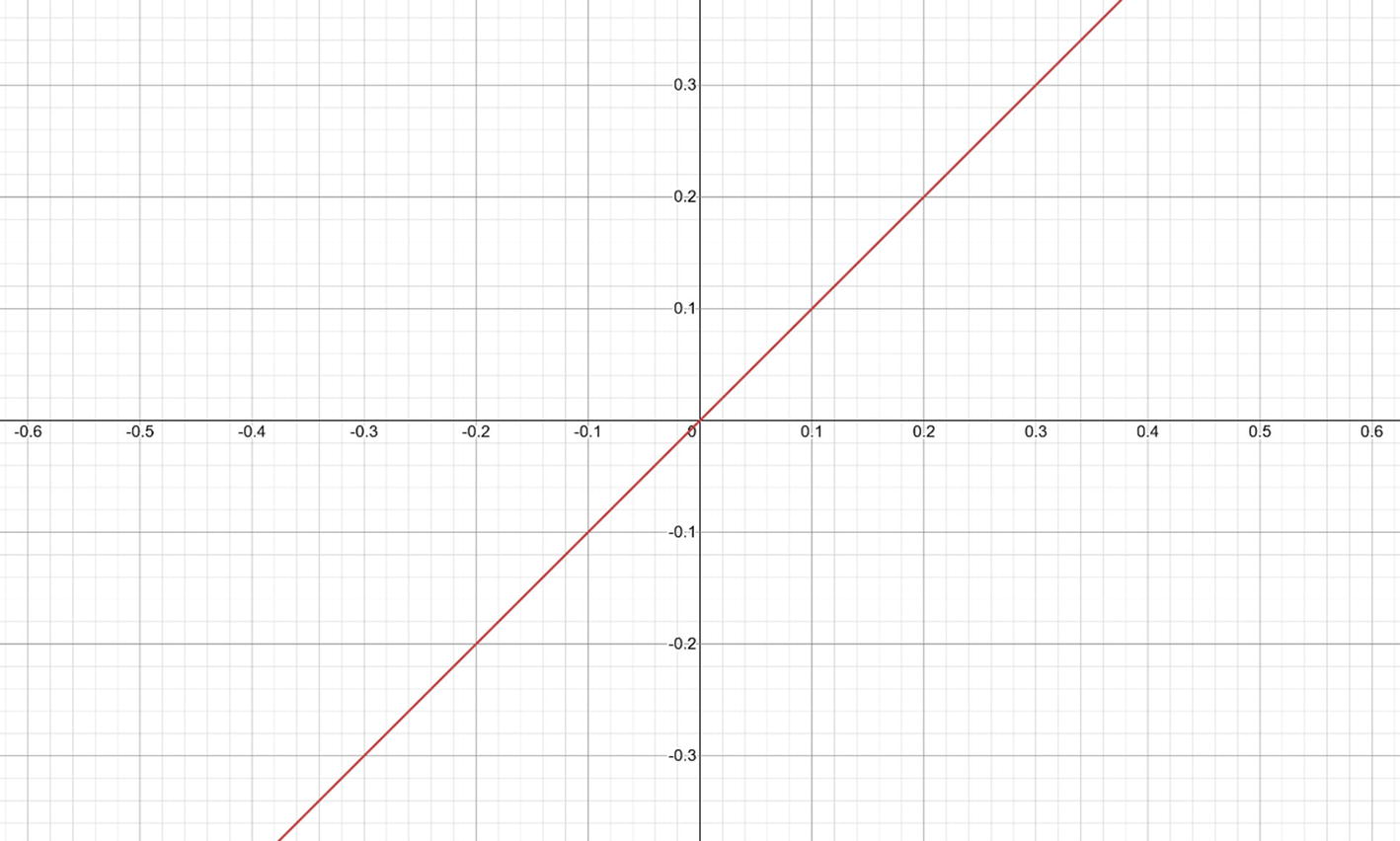
Figure 6-2.
A linear graph
Logarithms
Logarithms are a simple concept that people have made overly complex. We will begin our discussion of logarithms by discussing exponents.
An exponent is a way to represent a mathematical operation. An exponent consists of two numbers; one number is called the base, and the other is called the exponent or power, as in Figure 6-3.
Figure 6-3.
An exponent
The letter e has a special meaning in the realm of mathematics and by extension computing. e is known as Euler’s number, and it the base of natural logarithms. This important number is used in many applications from half-life calculations to economics and finance.
Figure 6-4 shows an exponential graph. This graph has a common plot and is easily recognizable.
Figure 6-4.
An exponential graph
At the core of many mathematical concepts lies a function or operation and its inverse. Consider the four basic mathematical operations of addition, subtraction, multiplication, and division. Addition is an operation whose inverse is subtraction, and similarly, multiplication is an operation whose inverse is division.
Since each of the basic operations has an inverse, it’s only fair that other complex functions also have inverses. For exponential functions, the inverse is the logarithm.
Logarithms are the reverse of exponents. To understand how this inverse works, we can look at the statement in Figure 6-5.
Figure 6-5.
Logs and exponents relationship
Logarithms find a lot of uses in computer science and engineering. As you will come to understand, many algorithms perform in a logarithmic manner. Figure 6-6 shows the logarithmic graph.
Figure 6-6.
A logarithmic graph
The logarithmic graph also has a distinctive shape, and this is something that you should learn and be able to recognize as you will encounter it throughout your study of DSA. At this point, we have a little understanding of linearity, exponents, and logarithms. With this knowledge, we begin our discussion of the searching algorithms
.
Linear Search
Searching for something seems like a trivial task for us. Let’s say that we have an array of elements from 1 to 10.
- [1, 2, 3, 4, 5, 6, 7, 8, 9, 10]
Now let’s say we wanted to find the number 7. How would we do that? Well, for us humans, it is easy to look at the array and simply see the number 7 and identify that it’s at index 6. For a computer, however, we must devise some algorithm to find the number 7. We could do something like this:
- 1.Have a variable that holds the number 7.
- 2.Loop through the array.
- 3.Compare each element in the array to our variable that stored the number 7.
- 4.If the variable matches an element in our array, we have found our number.
- 5.Return the index of the number we found.
This simple algorithm seems like a good way to find the number we need. In just five steps, we can find the index of the number we need. However, let’s say that we are looking for the number 10,000 in an array of numbers from 0 to 10,000. The time would increase significantly. In fact, if we keep adding elements to our array, the runtime will increase, and when we reach 10,000,000,000 numbers and we are looking for the number 9,999,999,999, the algorithm will seem like it isn’t running at all!
We call this type of algorithm a linear algorithm
having the notation O(n) since as the number of input elements increases, the runtime of the algorithm increases directly proportional to the increase in the number of elements. Think back to our talk on linearity, and you will realize that this is in fact a linear way of searching for an element.
The linear search is slow because it must scan all elements in the input to find the answer. For small array sizes, this may not be an issue; however, as the size increases, the algorithm slows down to the point where it will take hours or even days to find the number we are looking for.
However, there may be a situation where the linear search algorithm seems fast and may fool the uninformed programmer.
Let’s say our list of numbers is ordered as follows:
- [7, 5, 3, 10, 6, 2, 1, 8, 4, 9]
In this scenario, if we try to find the number 7 as we previously did, using the same algorithm, it will return a hit on the first try! The number 7 will be returned instantly! In fact, if we wrote our previous linear search algorithm and it gave such a result, we might be inclined to believe that the algorithm is instantaneous, having a time of O(1).
Don’t be fooled by this. The algorithm still has a time complexity of O(n). To prove this, let’s take the same array and swap the first and last elements.
- [9, 5, 3, 10, 6, 2, 1, 8, 4, 7]
Will the hit still be instantaneous? No, it will not, as the search algorithm will go through each element one by one until we find the one that we need. The time complexity will still be O(n) as the algorithm is still linear.
The linear searching not only can be applied to numbers but also to names, images, audio clips, and any type of data we may be working with. Searching is such an important thing that many algorithms have been devised to make searching as fast as possible for differing data structures.
While the linear search seems simple, it is inefficient. We will look at another searching technique that employs a logarithmic searching technique, the binary search.
Binary Search
While linear search is simple to implement, if suffers from one flaw. As the number of input elements to the searching algorithm increases, so too does the runtime of the algorithm increase. To combat this problem, a brilliant algorithm called binary search solves this problem.
We will learn how binary search works by walking through its method step-by-step.
Let’s say we have an array with numbers from 1 to 9.
If we were looking for the number 6, we could begin by identifying the center number of the array, which is 5.
- [1, 2, 3, 4, 5, 6, 7, 8, 9]
We will use the elimination method and eliminate numbers that are lower than our target number. To do this, we compare 5 to 6. Since 5 is less than 6, we know that the numbers less than 5, inclusive of 5, will not contain our target number. So, we eliminate 1, 2, 3, 4, and 5 until we are left with the following array:
- [6, 7, 8, 9]
Now that we have this array, we will repeat the process we previously did. We will try to locate the number 6. We find the center number of the array, which we identify as 7.
- [6, 7, 8, 9]
We compare the 7 with the number 6. Since 7 is greater than our target number, we know that any number larger than 7, inclusive of 7, would be too large. So, we can eliminate these numbers. We are left with this:
- [6]
After we perform the second elimination, we are left with our number that we wanted to find. We can then identify the index of the number we are looking for (since we know where it is) and return that index.
Though binary search seems like a longer and more involved method, it is actually a simple algorithm that is powerful.
We use the simple concept of taking an array, and we keep dividing that array in half and do a comparison to determine whether we have our target number.
The binary search is much more efficient than the linear search having a time complexity of O(log n). In fact, the algorithm is second in speed only to the constant time complexity O(1). Because as we know with logarithmic time complexity, as time increases linearly, then n goes up exponentially. This means that more elements will take less time to search.
When we are performing a simple search, the speed gains seem trivial. However, as we start performing more complex searching, the gains will be significant.
The only caveat with using binary search is that it works only if the array is sorted. If the array is not sorted, then binary search will not work.
With the power of binary search, you can perform a lot of searching tasks quite easily and in just a few steps. This algorithm is nice to use because it is both simple and powerful.
Conclusion
In this chapter, we got an introduction to algorithms, and we looked at two fundamental algorithms for searching, the linear search algorithm and the binary search algorithm. In the process of learning about these algorithms, we discussed the mathematical concepts of linearity and logarithms. In the subsequent chapters, we will discuss more algorithms that can be practically applied to your programs.