
In the previous chapter, we looked at an overview of data structures and algorithms. From this chapter forward, we will explore the types of data structures there are, beginning with the simple linear data structures. It is important to understand linear data structures because they get you into the mind-set of what a data structure is rather intuitively. If you have experience with data structures, you’ll like how simply the topic is presented. If this is your first time learning data structures, you’ll marvel at how simple they are to understand. This is the introduction I wish I had to the topic. Let’s get started with linear data structures!
Computer Memory
Before we delve into linear data structures, it is important to understand a little about computer memory. While it may seem unnecessary, remember that to understand data structures, we must understand a little of the underlying hardware, particularly memory organization.
Computer memory is to data structures as water is to a fish: it is essential for existence. As you will come to realize, the aim of many data structures is to effectively use the available resources, and one such resource is memory. Once we have a basic understanding of computer memory, we will be able to understand how linear data structures operate.
When we are talking about computer memory, we are talking about a type of workspace where the computer can store data that it is working on or has worked on. Essentially, memory is a storage space for the computer.
As a side note, something that we should know about memory is the terminology given to the binary prefix used to describe computer bits and bytes. We are all familiar with the terms kilobytes, megabytes, gigabytes, and terabytes that describe computer memory in terms of the metric system. Let’s take kilo, for example. In the metric system, kilo refers to 1,000; however, in the world of computing, when we say a kilobyte, we are usually referring to 1,024 bytes.
So, while in the usual context kilo means 1,000, in computing kilo would mean 1,024 since the International System of Units (SI) metric system did not have a way to represent units of digital information. Now, this is inconsistent, and within computer science, like all sciences, consistency in key. Thus, we refer to the units used in the SI system as the decimal prefix for describing measurement of memory.
To add some consistency, the International Electrotechnical Commission (IEC) units are now used when describing computer memory in some instances. The IEC units use a binary prefix
for describing memory as opposed to a decimal prefix. So, instead of byte
attached to the prefix there is now binary attached to the prefix.
This means that kilobyte (KB), megabyte (MB), and gigabyte (GB), for example, are now replaced with kilobinary (Ki), megabinary (Mi), and gigabinary (Gi). They are also referred to as kibibyte, mebibyte, and gibibyte as a contraction of their binary byte names. I use the IEC standards in this book when referring to memory size.
Computer memory is hierarchical, and this is important as each memory type on the machine is specialized. When we say something is hierarchical, we mean there is some order based on rank. In everyday life there are many hierarchical structures, and within computer memory there is no difference. Groups like the military and many systems in the natural world depend on a hierarchical structure for success.
Though there are many ways you can represent a hierarchical structure, a pyramid-based, stack-like structure is ideal for representing computer memory. A good way to visualize memory arrangement within a computing device is like the memory stack in Figure 2-1 where you have the largest memory on the bottom and the smaller memory on the top of the stack.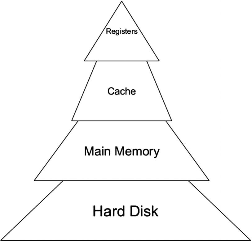
Figure 2-1.
Memory stack
This arrangement does not mean that any memory is more important than another as each component is necessary to make up the entirety of computer memory. Instead, this stack can be thought of as a sort of size hierarchy with the typical arrangement of the amount of memory that is typically present in a computing device.
If we look at our memory stack in Figure 2-1, we will see at the base of the structure is a hard disk. In computing devices, there is a storage device, which is typically a solid-state drive (SDD) or a hard disk drive (HDD), that we call disk storage or the hard disk. The hard disk is the component that contains the data that is loaded into main memory called random access memory (RAM).
The next layer of the stack is the RAM. RAM is called the main memory of the computer and is indeed the main memory of modern-day computing devices. RAM is further loaded into a type of memory called cache
that resides on the CPU chip. The information in cache is eventually loaded into the registers that contain data the CPU is presently working on.
Let’s say you are loading a word processing software. The software would reside on your hard disk memory. When you launch the program, it is transferred from the hard disk into RAM.
As you move up the stack from RAM, the next level you encounter is the cache memory. Within the cache there are generally two different caches; there is the L1 cache, which is fast and is almost as fast as the CPU registers (more on this later). There is also the L2 cache, which is slower than L1 but faster than RAM. Cache memory stores information that is most likely to be used by the CPU, making some operations extremely fast.
Cache is small, not exceeding a few mebibytes, and generally is in the kibibyte range. L1 cache is typically a few tens to just over 100 KiB, and L2 cache is a few hundred kibibytes.
Some CPU manufacturers also have an L3 cache, which is a few mebibytes. While cache has many benefits, it becomes inefficient if it is too large. Part of the reason cache speeds up operations is that it is much smaller than RAM, so we locate information in the cache easily. However, if the cache is too large, it becomes like RAM and the speed benefits decrease.
The example many people use is that of a textbook and your book of notes. When you have a textbook, the 1,000+ pages of information can be summarized into useful notes you are most likely to use or information that is important to you. Should you rewrite all 1,000+ pages of information in your notebook, then the efficiency of the textbook will diminish.
At the top of the stack is the register. The register is as fast and as small as memory can get within a computing device. Registers
are memory locations that are directly built into the processor. They are blazingly fast, and low-level languages can directly access this type of memory.
Memory can also be arranged into a hierarchy by speed. In Figure 2-2 we see this memory speed hierarchy. Within this structure we see that disk memory is the slowest, and register memory is the fastest.
Figure 2-2.
Memory speed hierarchy
Within computer memory you often hear people talking about the memory locations called the memory address
. The memory locations are known as physical addresses, whereas the operating system can give programs the illusion of having more memory by providing memory mappings to these physical addresses. We call these mapped representations of actual physical locations virtual memory
. What all this means is that though the actual memory locations are finite and thus can be exhausted, the operating system can provide proper management of memory to ensure programs using the memory have enough to run properly.
As we said earlier, virtual memory is a representation of physical memory space. Virtual memory contains virtual addresses that specify the location in virtual memory our program is accessing. This virtual memory is divided into virtual pages, which are used by a page table that performs address translation of virtual page map addresses to physical addresses.
The addresses provided by the operating system to your program identify each of these virtual memory slots. When you ask the computer to store something, the operating system will check to see which slots are available and let you store it there. If you have no slots available, then you will get an error and your program will not run.
While this information may not seem to be useful, keep this arrangement in mind as we move forward with our discussion on linear data structures.
An Overview of Linear Data Structures
When we say that a data structure is linear, we mean the elements of which the data structure are comprised are arranged in such a manner that they are ordered sequentially, with the relationship between elements being an adjacent connection. Such structures are simple to understand and use when developing programs.
In this section, we will examine the most common of these linear data structures: the array and the list. These two linear structures are the two “workhorse” data structures because almost all other data structures stem from them or use them in some way.
Once you understand the array and list, you will have a solid foundation to begin working with other data structures. While they may have different names in other programming languages, the purpose and arrangement will be similar and will serve you well no matter which language you are using.
The Array
The array
is one of the most fundamental data structures we have for storing and organizing data. It is such a basic data structure that it usually is part of the underlying programming language. All the popular C-based programming languages utilize arrays, so you are sure to encounter them. As simple as arrays are, they are powerful and the best starting point for any discussion on data structures.
Arrays store elements that are of the same data type. In Chapter 1, we discussed the different data types, and should you need a refresher, you can refer to that chapter. We call each of these data types an element, and the elements are numbered starting from 0.
The number assigned to an element is called the index of the array. The array has a structure like Figure 2-3, with elements arranged sequentially. These elements usually have commas separating them. This is how arrays are represented in many of the C-based programming languages, and this is the convention we will use in this book.
Figure 2-3.
The array structure
If we think about the arrangement of elements within the array, we will see that the elements within the array are arranged sequentially or consecutively. Because of this sequential nature, data in an array can be read randomly. However, adding and deleting data from an array can take a lot of time due to this sequential organization of elements. This is one of the limitations of the array as a data structure. There are others, as you will uncover as we go along; however, this is a prominent one.
In most programming languages, when the computer is assigning memory for an array, the size of the array must be specified by the program designer before memory is allocated for the array. This means the programming language lets you reserve the size of the array before the program is run. Other programming languages provide mechanisms by which you do not need to explicitly reserve any memory, which saves memory space and leaves less burden on the programmer.
The type of arrays we described previously is called a one-dimensional array. We call it a one-dimensional array because when you access elements from within the array, it is a single element you are accessing at each index, representing either a single row or a single column.
An array may also be multidimensional. A multidimensional array can be thought of as an array of arrays. Such structures are useful when you want to define something as a grid, since two-dimensional arrays are essentially a grid of rows and columns that you can access programmatically. The most commonly used multidimensional array is the two-dimensional array. When we store data in a two-dimensional structure, it is known as a matrix
.
Lists
The list can be thought of as a special type of array. Whereas in an array data is stored in memory sequentially, in the list data is stored disjointed in memory. This allows for a linked list to utilize memory more effectively.
In a list, the data is organized in such a way that each data element is paired with a pointer or reference that indicates the next memory location for the next element within the list. To access a data element, we must access it through the pointer that precedes it.
The pair of a data element and a pointer to the next item in the list is known as a node. The list is structured in that there is an entry point into the linked list. This entry point is called the head of the list.
This type of linked list structure with one node having a pointer to the other is known as a singly linked list. In the singly linked list, the last node doesn’t point to any other node and has a null value. Figure 2-4 gives a good representation of the linked list data structure.
Figure 2-4.
The linked list data structure
There is also a linked list structure where each node has a pointer not only to the next node in the list but also to the previous node in the list. This layout is called the doubly linked list. Figure 2-5 shows the doubly linked list. This layout makes the linked list more efficient when deleting data and for allowing bidirectional traversal of the list.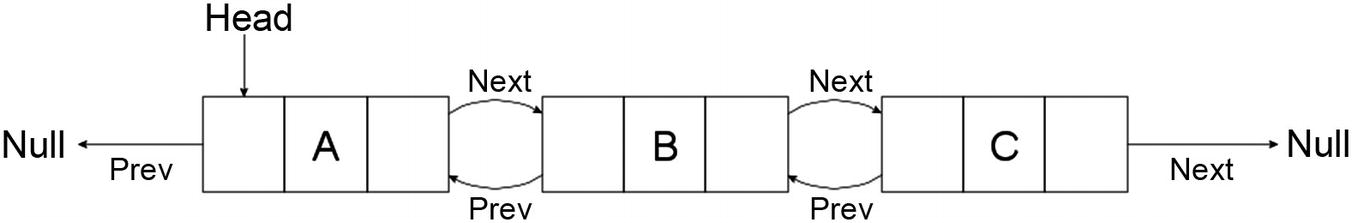
Figure 2-5.
The doubly linked list data structure
Lists may also be of the type called a circular linked list
. In a circular linked list, all the nodes are connected to form a circular arrangement. The last node is connected to the first node, and there is no null at the end of the list.
The internode connections within a circular linked list may be either singly linked or doubly linked. Figure 2-6 shows us what a circular singly linked list looks like.
Figure 2-6.
Circular singly linked list
These circular linked lists have many uses within computing, particularly uses related to buffering and other creative uses the programmer comes up with. Circular lists can also be used for queues, which is something we will look at later in this chapter.
Stacks
Stacks
are a type of linear data structure where the data that is added is put into the lowest available memory location. Stacks are abstract in that we think of how they operate, but their implementation will vary based on the technology used to implement the stack and on the type of stack we are trying to construct.
The act of adding data to the stack is called a push. When we remove data from the stack, we do so by removing the element that was last added; this is called a pop. Because of this arrangement of removing data first that was last added to the stack, we call the stack a last in first out (LIFO) data structure. Figure 2-7 shows us the arrangement of the stack.
Figure 2-7.
The stack
While this concept is simple to visualize, one of the key weaknesses of the stack as a data structure is in its simplicity. The stack can have data elements removed and added only from the top of the stack. This limits the speed at which a certain element can be retrieved from the stack. However, in applications such as reversing a string or backtracking, for example, the stack can be useful.
We can create stacks that are static, meaning they have a fixed capacity, and we can create stacks that are dynamic, meaning the capacity can increase at runtime. Dynamic stacks vary not only in size but also in the amount of memory they consume.
To create a static stack, we can use an array. We can also design a stack that is dynamic by using a singly linked list with a reference to the top element, which is why earlier I mentioned that while the operation of the stack will remain the same, the implementation will vary. Stacks find uses in many fundamental computing processes including function calls, scheduling, and interrupt mechanisms
.
Queues
A queue
is a type of data structure that assigns a priority to each element. Elements that are added first to the queue are placed at the end of the queue. The act of adding data to a queue is known as enqueue
. When we are removing a data element from the queue, the element that has been in the queue the longest is removed first. When we extract data from a queue, we call it a dequeue.
Because of the queue removing data that was added to the queue first, we say that the queue is a first in first out (FIFO) data structure. This can be contrasted with the last in first out (LIFO) nature of stacks.
By combining the LIFO structure of stacks with the FIFO structure of queues, we can create some pretty amazing programs and structures, as we will see later in the book.
The queue is unique in that although the basic queue as we discussed here is a linear data structure, there are some queues that can take a nonlinear form, as we will discuss later.
In Figure 2-8 we see the FIFO method in action. New items are added to the rear of the queue for the enqueue, and requested items are removed from the front of the queue for the dequeue.
Figure 2-8.
Queue
Priority Queues
A priority queue
is an extension of the regular queue we discussed earlier. The priority queue, however, uses a key-value system to arrange the items within the queue. In the priority queue, every item in the queue has a priority associated with it, which can be thought of as a key. An element within the priority queue with a higher priority will be dequeued before an element with a lower priority. If we have two elements within the priority queue that have the same priority within the queue, they will be dequeued according to their order within the queue.
Sometimes items within a priority queue may have the same priority; when this occurs, then the order of the items within the queue is considered. When using priority queues, these data structures usually have methods to add items to the queue, delete items from the queue, get items from the queue with the highest priority, and check if the queue is full, among other things.
These queues can be constructed using the other data structures we examined such as linked lists and arrays. The fundamental data structures we use to construct the queue can affect the properties of the queue.
Priority queues enqueue items to the rear of the queue and dequeue items from the front of the queue. Figure 2-9 shows the priority queue.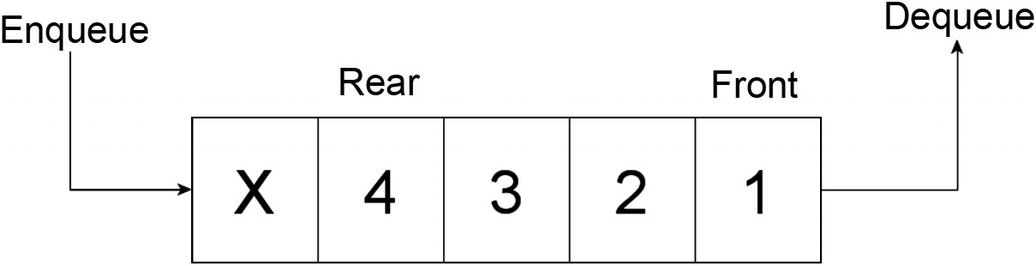
Figure 2-9.
Priority queue
As we will see later, some algorithms will utilize priority queues, which have many uses in data compression, networking, and countless other computer science applications.
Conclusion
In this chapter, we looked at various linear data structures. We discussed the basics of computer memory, arrays, linked lists, stacks, and queues. While this introduction was compact, we covered a lot of information without dwelling too much on unnecessary implementation details. These basic data structures have many applications that we will see moving forward. In the next chapter, we will look at trees, which will advance your understanding of data structures.