A.1 Essential Mathematical Background

In this section, we consider the mathematical background needed generally in computer science and specifically in study of Formal Languages and Theory of Automata, for those students who do not have it or who want to revise.

Why do we need mathematics at all in computer science?

• To present information in an easily assimilated form;
• To provide a convenient method for solving a problem;
• To predict the behaviour of a real system.

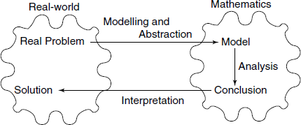
In short, we use mathematics to model the real-world, see Fig. A .1.

 

A.1.1 Formal Logic: A Language for Mathematics

In many situations, we have to represent and deal with statements describing some real-world fact or event. We should be able to express such information and process it precisely. A branch of mathematics, Formal Logic, is concerned with this requirement. There are several areas in logic.

• Classical logic
  • Propositional logic
  • Predicate logic
• Non-classical logic
  • Modal logic
  • Multi-valued logic
  • Fuzzy logic, etc.

We are concerned here with Propositional and Predicate logic.

 

Table A.1 Examples: assertions

Assertion	Assertion?	Proposition?
3 is not an even integer	Yes	True
4 is a prime number	Yes	False
The square of an integer is non-negative	Yes	True
The moon is made of blue cheese	Yes	False
x is greater than 5	Yes	No
This statement is false	Yes	No
Is he a CS student?	No	No
How are you?	No	No
What a difficult problem it is	No	No
Write this program	No	No

A.1.2 Assertions and Propositions

First, we take some definitions:

Assertion: A statement (i.e., a declarative sentence).

Proposition: An assertion which is either true or false, but not both.

Truth value: Whether a proposition is true or not.

Note that whether a proposition is true is not necessarily known. For example, “A meteorite landed on the Chowpati, Mumbai, in 258 BC” is a proposition.

In order to deal with propositions systematically and study their structures, propositions are often denoted by symbols, say P, Q, R, etc., which are called propositional variables. Note that such variables take truth values – True or False. A truth table of a proposition P including k propositional variables is a table which shows the truth value of P for each combination of truth values of the propositional variables.

A.1.3 Logical Connectives

The real-world situations almost always need to be expressed as a combination of facts. In propositional logic, this is modelled by a compound proposition.

A compound proposition is constructed from existing propositions by applying operators called logical connectives.

Negation – NOT operation

Notations: NOT ¬ ∼

Definition (given by a truth table):

P	NOT P
T	F
F	T

T and F denote True and False, respectively.

This operation is used to show absence of some condition or fact. For example, if P denotes “today is Monday”, then ¬ P denotes “today is not Monday” or “today is other than Monday”.

Conjunction – AND operation

Notations: AND ∧.

Definition:

P	Q	P ∧ Q
T	T	T
T	F	F
F	T	F
F	F	F

This connective denotes that both of the two propositions are True.

Disjunction (Inclusive) OR Operation

Notations: OR ∨ +

Definition:

P	Q	P ∨ Q
T	T	T
T	F	T
F	T	T
F	F	F

This connective denotes that either one or both of the two propositions are True.

Examples

Gopal is at school and either Mani is on the phone or Sita is at the store.

Let G denotes “Gopal is at school”, M denotes “Mani is on the phone”, and S denotes “Sita is at the store”.

The above compound proposition is denoted by G ∧ (M ∨ S). Note that parentheses are used to avoid ambiguity in expressions.

Then, (¬ M) ∧ (¬ (G ∨ S)) denote the following: Mani is not on the phone and it is not the case that either Gopal is at school or Sita is at the store.

Exclusive OR

Notations: XOR ⊕ ^

Definition: Note that P ⊕ Q has the same truth table as (P ∨ Q) ∧ ¬ (P ∧ Q).

This connective denotes that one and only one of the two propositions is True.

P	Q	P ⊕ Q
T	T	F
T	F	T
F	T	T
F	F	F

Conditional or Implication

Notations: →

Definition:

P	Q	P → Q
T	T	T
T	F	F
F	T	T
F	F	T

Note that P → Q has the same truth table as (¬ P) ∨ Q.

The left-hand side of → is called a hypothesis or premise and the right-hand side is called a conclusion or consequence.

Q → P is called the converse of P → Q. ¬ P → ¬ Q is called the contra-positive of P → Q.

Biconditional or Equivalence

Notations: ↔ ⇔

Definition:

P	Q	P ↔ Q
T	T	T
T	F	F
F	T	F
F	F	T

Note that P ↔ Q has the same truth table as (P → Q) ∧ (Q → P).

A conditional statement P → Q may correspond to the following in a natural language:

If P, then Q;

P only if Q;

P implies Q;

When P, Q;

P only when Q;

P is a sufficient condition for Q;

Q is a necessary condition for P;

Q if P;

Q follows from P;

Q, provided P;

Q is a logical consequence of P;

Q whenever P; etc.

A bidirectional statement P ↔ Q may correspond to the following in a natural language:

P if and only if Q;

P is equivalent to Q;

Q is equivalent to P;

P is a necessary and sufficient condition for Q;

Q is a necessary and sufficient condition for P.

Tautologies, Contradictions and Contingencies

Tautology A proposition which is always true.

Example: (P → Q) → (( ¬ Q ) → (¬ P))

In the truth table of a tautology, every row has T.

Contradiction A proposition which is always false.

Example: (P → Q) ∧ (P → ( ¬ Q )) ∧P

In the truth table of a contradiction, every row has F.

Contingency A proposition which is neither a tautology nor a contradiction.

Example: (P → Q) → (Q → P)

In the truth table of a contingency, some rows have T and the others have F.

Implementation Notes

Most programming languages, including C, provide for expressing predicates in the form of IF (condition) THEN statement-T ELSE statement-F. It is important to note that though seemingly such a construct implements p ⇔ q If and only If, it is really p ⇒ q, i.e. If p then q, because q may be true or false before execution of a statement “IF(p) THEN q”, but afterwards, q will be true if p is true. If you want the if-and-only-if behaviour, you must use “IF(p) THEN q ELSE not q”.

One very important facility in C related to predicates is the assert() function, which checks any given assertion and terminates the program if it is not true, giving an error diagnostic. This facility seems to have escaped the attention of most of academic institutions, but it is important from viewpoint of debugging real-life programs.

A.1.4 Sets

A set is a collection of entities that can be identified. The entities are called members or elements of the set. Sets are characterized by the concept of membership, denoted by the symbol ∈.

 

 

 

A set can be Finite, for example, the set of non-negative integers less than 5.

A small finite set is often written out fully as, for example {1, 2, 3, 4}.

A set can be Empty, for example, a set of all human beings aged more than 500 years. Such a set is also called null-set and denoted by symbol Ø.

A set can be Infinite, for example, the set of all C programs. This is not a finite set, since no matter how large a program you write, it is possible to write a larger one by inserting another statement.

A set can have other sets as its elements, for example, S = {1, 2, {a, b}}. Here, note that element a is not a member of set S, but rather member of anonymous set {a, b}, which is member of S.

Notations for Sets

Usually, two notations are used to specify sets:

• Enumeration: for example {0, 1, 2, 3, 4}
• Set-builder form; or, Predicate form:

{x | P(x)}               where P(x) is a predicate that describes a property of all elements x

{x ∈ S | P(x)}        equivalent to {x | x ∈ S ∧ P(x)}

For example, {x | x is an integer ∧ 0 ≤ x ∧x < 5}

 

There are a few sets used so often that they are called Special Sets:

 

ℕ: The set of natural numbers (usually including 0)

ℤ: The set of integers

ℚ: The set of rational numbers

ℝ: The set of real numbers

ℂ: The set of complex numbers

ℤ₊: Also ℙ, the set of positive integers

ℤ_n: The set of non-negative integers less than n

ℝ₊: The set of positive real numbers

Relationships Between Sets

Let X and Y be arbitrary sets.

 

X is a subset of Y, denoted as X ⊂ Y, iff ∀ x (x ∈ X) → (x ∈ Y) holds.

Y is a superset of X iff X is a subset of Y.

X and Y are equal, denoted as X = Y, iff X ⊂ Y and Y ⊂ X.

X ≠Y denotes that X and Y are not equal.

X is a proper subset of Y iff X ⊂ Y and X ≠ Y.

X and Y are said to be (mutually) disjoint iff no element is in both X and Y.

Set Operations

Let U denote the universal set that is the common set from which elements of sets are selected. The following operations on sets are defined:

Union: A ∪ B = {x|x ∈ A ∨ x ∈ B}

Intersection: A ∩ B = {x | x ∈ A ∧ x ∈ B}

Complement: A = {x ∈ U | ¬ (x ∈ A)}

Set dIfference: A – B = {x | x in A ∧ ¬ (x ∈ B)}. Note that A – B is not equal to B – A in general.

Cartesian product: A × B = {(x, y) | x ∈ A ∧ y ∈ B}. Elements in a Cartesian product are called ordered tuples.

Power set: For a set A, 2^A = {B | B ⊂ A}. This is the set of all subsets of A. Some textbooks denote the power set by P(A).

Notation: The union of a number of sets is denoted by

 

 

Similarly, intersection of a number of sets is denoted by

 

 

Properties of Sets

Sets obey the following algebraic laws:

Here, U denotes the universal set.

• Idempotent law: A ∪ A = A, A ∩ A = A
• Associative law: (A ∩ B) ∩ C = A ∩ (B ∩ C), (A ∪ B) ∪ C = A ∪ (B ∪ C)
• Commutative law: A ∩ B = B ∩ A, A ∪ B = B ∪ A
• Distributive law: A ∩ (B ∪ C) = (A ∩ B) ∪ (A ∩ C), A ∪ (B ∩ C) = (A ∪ B) ∩ (A ∪ C)
• Absorptive law: A ∩ (A ∪ B) = A, A ∪ (A ∩ B) = A
• Identity law:
• Complement law:
• DeMorgan's law:

Sets – Implementation Notes

Theory of sets forms bases of many designs – both hardware and software in computer field. They are used extensively in design of language translators. How do we represent sets in a computer? It depends upon the nature of elements in the set, size of the set and what operations we are going to perform on them in our application.

A set can be represented as:

• an array – limited size, same type of elements, fast operations;
• a linked list – arbitrary size, slow operations;
• a bit field – most useful for limited size, very fast operations;
• a hash table – arbitrary size, reasonably fast operations.

All the four methods can be used in C language, but bit-field method is the fastest and most economical in memory if large sets are to be handled. If the sets we want to handle are all of size 32 or less, then we can use an unsigned integer to represent it, each bit position representing inclusion of a particular element in the set. For example, suppose our universal set has 32 elements {1, 2, …, 32}. Let set A = {1, 3, 6} and set B = {3, 4, 5, 6}. A will be represented as 0…0100101 = 00000025 (hex), and B as 0…0111100 = 0000003C (hex).

Union, intersection, negation and Ex-OR are very easy with this representation.

Union: Use logical OR operation, ‘|’, e.g. A ∪ B = 00000025 | 0000003C = 0000003D → {1, 3, 4, 5, 6}.

Intersection: Use logical AND operation, ‘&’, e.g. A ∩ B = 00000025 ‘&’ 0000003C = 00000024 → {3, 6}.

Negation: Just take complement by ‘∼’ operation.

Ex-OR: Use logical Ex-OR operation, ‘∧’.

Existence of a member: To check if member number i is in the set, use the expression (set &

(1 «(i – 1))).

One limitation of this method is that it is difficult for cases where we have to handle mixed sets, like set of sets.

Can we use this technique for larger set sizes? Yes, for details see p. 690 [Hol90]. Elsewhere we have given a number of example programs for checking of grammars etc., which uses a different implementation for sets and set operations, for the reason indicated above. In anticipation of that development, we give here our implementation of a set. See C code files set.h and set.c.

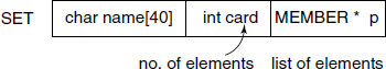
Each member of a set is represented by a data structure shown in Fig. A .2 and a set is represented by a data structure shown in Fig. A .3. A number of processing functions like union, intersection, etc. are provided.

 

 

 

In Perl and Python, it is easiest to use Hashes or Dictionaries for implementing sets. Simplest representation would be:

$myset{able} = 1;
$myset{baker} = 1;

i.e., just add hash members with element names as key and ‘1’ as value. If more information for each element is needed to be stored, then references can be used in place of ‘1’ as the value.

 

Functions

Let X and Y be sets.

A partial function f from X to Y, denoted f X→ Y, is a subset of X × Y (i.e., the Cartesian product of X and Y) which satisfies the condition that for each x ∈ X, there is at most one y ∈ Y such that (x, y) ∈ f.

X is called the domain of f and Y is called the range (or codomain) of f

Notation: f(x) = y iff (x, y) ∈ f

 

x is called an argument of f and y is the value of f for x.

f(x) is undefined if there is no y such that (x, y) → f.

A partial function/: X → Y is called a total function (or simply function) if ∀x ∈ X, there is one and only one y ∈ Y such that f(x) = y.

Operations on Functions

Let g: X→ Y and f Y→Z be functions. The composition of f and g, written as f ο g, is a function from X to Z such that ∀ x ∈ X, (f ο g)(x) =f(g(x)).

Composition of functions is associative. If f, g and h are functions, then (f ο g) ο h (= f ο (g ο h).

The inverse of f: X → Y is a function g: Y → X such that ∀ x ∈ X, (g ο f)(x) = x.

Note that the inverse of f does not necessarily exist.

Notation: f⁻¹ denotes the inverse of f if it exists.

Classification of Total Functions

Surjection f: X → Y is surjective (or onto) Iff f(X) = Y

Injection f: X → Y is injective (or one-to-one) iff x ≠ x’ implies(fx) ≠ f(x’). This means that if f(x) = f(x’), then x = x’.

Bijection f: X→ Y is bijective (or one-to-one correspondence) iff f is both surjective and injective.

Theorem A.1.1 A function f is bijective Iff f⁻¹ exists.

Cardinality of a Set

Let S be a set and let ℤ_n = {0, 1, 2, 3, …, n – 1}.

S is a finite set of cardinality n iff there is a bijection f: ℤ_n → S. We write |S| = n.

S is infinite iff S is not finite.

S is countably infinite iff there is a bijection f: N → S, where N is the set of natural numbers 0, 1, 2, …. The cardinality of a countably infinite set is called א₀, pronounced “aleph zero”.

S is said to be countable if S is finite or countably infinite. S is said to be uncountably infinite (or uncountable) if there is no bijection f: N → S.

Theorem A.1.2 The set R of real numbers is uncountably infinite.

This theorem is usually proved by a process known as Diagonalization. For further details, see Section A.1.9.

Two sets A and B are said to have the same cardinality if there is a bijection between A and B.

If there is a bijection f: R → S, where R is the set of real numbers, the cardinality of S is called א₁.

Implementation Notes

Almost all modern programming languages provide for definition and use of functions.

A.1.5 Relations

Cartesian Product (Cross Product)

A × B = {(x, y) | x ∈ A ∧ b ∈ B}. Here the ordered pairs are sometimes denoted by <x, y>

 

 

The ordered n-tuple (x₁, x₂, …, x_n ) is sometimes denoted by < x₁, x₂, …, x_n >.

An n-ary relation R among A₁, A₂, …, A_n is a subset of A₁ × A₂ × … × A_n.

R = {(x₁, x₂, …, x_n ) | P((x₁, x₂, …, x_n)) ∧ x_i ∈ A_i ∀i, (1 ≤ i ≤ n)} where P is a predicate representing properties of R. n is called the arity of R.

If n = 2, R is called a binary relation from A₁ to A₂. A₁ is called a domain and A₂ is called a range or codomain.

If A = A₁ = A₂ = … = A_n, R is called a relation on A.

For example,

Let P(x, y, z) denote “student x has been studying y for z years”. X = a set of all students; Y= a set of majors; Z = a set of positive integers.

 

Binary Relations and Digraphs

We now focus on binary relations on a set A.

Notation: (x, y) in R iff xRy, i.e. x is R-related to y

Graphical Representation

 

 

an element in A is equivalent to a vertex (or node) and an element in R is equivalent to an edge (or arc).

These two sets form what is known as a Directed graph (digraph for short), denoted by G = (V, E), where V is a set of vertices and E is a set of edges which are ordered pairs of vertices (see next section).

Classification of Binary Relations

Let R be a binary relation on a set A.

• R is reflexive iff (x, x) ∈ R ∀ x ∈ A
• R is irreflexive iff (x, x) ∉ R ∀ x ∈ A. Note that R can be neither reflexive nor irreflexive.
• R is symmetric iff (x, y) ∈ R → (y, x) ∈ R ∀ pairs x,y ∈ A.
• R is antisymmetric iff (x, y) ∈ R and (y, x) in R → x = y ∀ x and y ∈ A. Note that R can be both symmetric and antisymmetric, and R can be neither symmetric nor antisymmetric.
• R is transitive iff (x, y) ∈ R and (y, z) ∈ R → (x, z) ∈ R → triple of x,y and z ∈ A.

Relations Types in Digraph Representation

Reflexive: Every vertex has a self-loop.

Irreflexive: No vertex has a self-loop.

Symmetric: If there is an edge from one vertex to another, there is an edge in the opposite direction.

Antisymmetric: There is at most one edge between distinct vertices.

Transitive: If there is a path from one vertex to another, there is an edge from the vertex to another.

Operations on Relations

Because a binary relation R is just a set of pairs drawn from the basic sets A and B, the set operation like Union, Intersection, Set Difference, Complement, Inverse (or Converse) are defined on a pair R₁, R₂ of them. Further, let R₁ be a binary relation from A to B and R₂ be a binary relation from B to C. Then the operation of composition is defined on them as:

R₁ ο R₂ = {(x, z) | ∃ y, [(x, y) ∈ R₁ ∧ (y, z) ∈ R₂]} which is a binary relation from A to C. This relation has properties of Associativity and Distributivity over union.

Let R be a relation on A. The n-th power Rⁿ is identity relation defined as {(x, x) | x ∈ A} if n = 0; and is Rⁿ⁻¹ R If n > 0.

The Transitive Closure of a relation is defined as:

Equivalence Relations and Equivalence Classes

Let R be a binary relation on A. Then R is an equivalence relation on A Iff R is reflexive, symmetric and transitive.

For example,

Let Z be the set of integers, and n be a positive integer. Let R = {(i, j) | i ≅ j (mod n)}, i.e. R = {(i, j) | ∃ k, [kn = i – j]}.

Then,

1. R is reflexive, since i ≅ i (mod n) ∀i ∈ Z.
2. R is symmetric, since i ≅ j (mod n) implies j ≅ i (mod n).
3. R is transitive.

Partitions

Let X be a set of subsets S₁, S₂ …, S_m of A.

X is called a partition of A iff

1. and
2. S_i ∩ S_j = Ø ∀ 1 ≤ i ≤ m, 1 ≤ j ≤ m and i ≠ j, m is called the rank of X.

Order Relations

An order relation is a transitive binary relation on a set A. A partial order on A is a reflexive, antisymmetric, transitive binary relation on A. The ordered pair (A, R) is called a partially ordered set or poset. Elements x and y in A are said to be comparable iff either xRy or yRx holds.

A partial order R on A is called a total order on A iff for every pair x and y in A, x and y are comparable.

The ordered pair (A, R) is called a totally ordered set.

For example,

The relation “less than or equal to” on the set of natural numbers:

• Reflexive: For every i ∈ N, i ≤ i holds.
• Antisymmetric: For every i and j (i ≠ j), exactly one of i < j and j < i holds.
• Transitive: If i ≤ j and j ≤ k hold, then i ≤ k holds.

Thus, ≤ is a partial order on N.

A.1.6 Inductive Definitions

Recursive definition in more general is called Inductive Definition.

Let S be an infinite set to be defined.

An inductive definition of S consists of the following three components:

Base Clause (or Basis): To establish that a finite number (usually one) of certain objects are elements in the set S;

Inductive Clause (or Induction): To establish a way to obtain a new element from some of the previously defined elements of the set S;

Extremal Clause (sometimes left implicit): To assert that unless an object can be shown to be an element of the set S by applying the base and inductive clauses only a finite number of times, the object is not an element of S.

Example: Even Integers

Suppose that the universe is the set of integers. The set E of even integers can be defined inductively as follows:

1. Base Clause: 0 ∈ E.
2. Inductive Clause: If x ∈ E, both of x + 2 and x – 2 are in E .
3. Extremal Clause: No integer is in E unless it can be shown to be so by a finite number of applications of Clauses (1) and (2).

Example: Power Set

Let A be a set. The power set 2^A (i.e., the set of all subsets of A) can be inductively defined as follows:

1. Base Clause: The empty set Ø ∈ 2^A .
2. Inductive Clause: If X ∈ 2^A and w ∈ A, then the union X ∪ {w} ∈ 2^A .
3. Extremal Clause: Nothing else in 2^A other than sets obtained by applying (1) and (2) a finite number of times.

A.1.7 Proof Techniques

First, we consider some definitions:

Axiom: An assertion that is assumed to be true.

Hypotheses: An assertion proposed as a theorem

Theorem: An assertion that can be shown to be true.

Pro of: An argument to establish the truth of a theorem.

Inference rules: A means of deducing a theorem from axioms and/or previously proved theorems.

There is no general algorithm for deducing systematically whether a given assertion is true or false.

The construction of proofs is an art and a craft. The skill to develop a proof can only be learned by means of examples and practice.

Generally, a proof consists of a series of assertions from which the final assertion is derived and that is the Conclusion – the assertion to be proved. For example, a typical inference rule is:

if P → Q and

Q → R then

P → R (conclusion)

There are a number of such Inference Rules which help us in developing a proof. Some of them are:

if P then P ∨ Q , can also be written as P ⇒ P ∨ Q

if P ∧ Q then P

if P, P → Q then Q this rule known as Modus Ponens

if ¬ Q , P → Q then ¬ P Modus Tollens

if P ∨ Q , ¬ P then Q

if P, Q then P ∧ Q

if P → Q, R → S, P ∨ R then Q ∨ S

if P → Q , R → S, ¬ Q ∨ ¬ S then ¬ P ∨ ¬ R

Various Proof Methods

Vacuous Proof (P → Q ) is true if P is false.

Trivial Proof (P → Q ) is true if Q is true.

Direct Proof: Assume that P is true. Show that Q must be true, by applying inference rules.

Proof of the Contrapositive: Show that the contrapositive (( ¬ Q) → ( ¬ P)) of (P → Q ) is true, by using other proof techniques.

Proof by Contradiction: Assume that (P → Q ) were false, i.e. P were true and Q were false. Derive a contradiction such as (R ∧( ¬ R)) from this assumption, by applying inference rules.

Reduction to Absurdity: Assume that (P → Q ) were false. Derive ( ¬ R) from this assumption for a known theorem R.

A.1.8 Proof by Induction

The concept of induction provides not only a method of defining infinite sets, but also powerful techniques for proving assertions of the form ∀x, P(x), where the universe is an inductively defined set (e.g., the set of natural numbers).

A proof by induction usually consists of two parts corresponding to the base and inductive clauses of the definition of the universe S.

Base Step (or Basis) to establish P(x) is true for every element x specified in the base clause of the definition of S.

Inductive Step (or Induction) to establish that P(x) is true for each element x constructed in the inductive clause of the definition of S, assuming that P(y) is true for all the elements y used in the construction of x. This assumption is called Induction Hypothesis.

Note that there is no step corresponding to the extremal clause of the definition of S. Since the extremal clause in the definition of S guarantees that all elements of S can be constructed using only the base and inductive clauses a finite number of times, P(x) holds for all elements of S.

For example,

Let the alphabet ∑ = {( , )}. A set B of strings over ∑ is the subset of ∑⁺ such that

1. Basis: ( ) ∈ B.
2. Induction: If x and y ∈ B, then (x) and xy ∈ B.
3. Extremal: B consists of all strings over ∑ which can be constructed by a finite number of applications of (1) and (2).

Theorem A.1.3 Let L(x) denote the number of left parentheses in x ∈ B and R(x) denote the number of right parentheses in x ∈ B.∀ x, L(x) = R(x).

Proof by Induction:

1. Basis: x = ( ) ∈ B, since L(x) = 1 and R(x) = 1, L(x) = R(x) holds.
2. Induction: Assume that L(x) = R(x) and L(y) = R(y) for x and y ∈ B.

   Case 1: Consider (x) in B. L((x)) = L(x) + 1 R((x)) = R(x) + 1

   By induction hypothesis, L(x) = R(x), L(x) + 1 = R(x) + 1. Hence, L((x)) = R((x)) holds.

   Case 2: Consider xy in B. L(xy) = L(x) + L(y) R(xy) = R(x) + R(y)

   By induction hypothesis, L(x) + L(y) = R(x) + R(y). Hence, L(xy) = R(xy) holds.

   Therefore, L(x) = R(x) holds for all x in B.

First Principle of Mathematical Induction

Suppose that the universe is the set of natural numbers N = {0, 1, 2,…}. Let P(n) be a predicate on N.

Inference Rule: Given P(0); if ∀ n, P(n) → P(n + 1) then ∀ n, P(n).

Proof Technique:

1. Basis: Show that P(0) is true, using whatever proof technique is appropriate.
2. Induction: Let n be an arbitrary element in the universe. Assume that P(n) is true (induction hypothesis). Show that P(n + 1) is true.

For example,

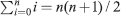
To prove:

Here,

Proof: Induction on n

1. Basis: n = 0 LHS RHS = 0(0 +1) / 2 = 0. Thus, the equality holds. Hence, P(0) is true.
2. Induction: Assume that P(n) is true, i.e. holds. Consider P(n + 1). 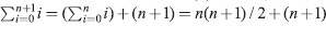by induction hypothesis = (n + 1)(n + 2)/2. Hence, P(n + 1) is true.

One has to be careful in applying the principle of inductive proof, otherwise a wrong proof can result.

Second Principle of Mathematical Induction

Inference Rule: If ∀ n, [∀ k, k < n → P(k)] → P(n) then ∀ n, P(n).

Proof Technique: Let n be an arbitrary element in the universe. Assume that for every k < n, P(k) is true. Show that P(n) is true.

This proof technique is more powerful than the first principle of mathematical induction.

For example,

To prove: All integers n ≥ 2 can be written as a product of prime numbers.

Here, P(n) = “n can be written as a product of primes”.

Proof: Induction on n ≥ 2

Assume that ∀ k such that 2 ≤ k < n, k can be written as a product of primes. We will show that n can be written as a product of primes. The proof is by cases.

 

Case 1: n is a prime. Then n is such a product of one prime that is itself.

Case 2: n is not a prime. Then n must have a factor i, where 2 ≤ i ≤ n. Thus, we can write n = ij, where 2 ≤ j ≤ n. By the induction hypothesis, both i and j can be written as products of primes. Thus, n can be written as a product of the products of primes.

In both cases, P(n) is true.

Note that this cannot be proved by the first principle of mathematical induction.

Proof by Induction is used in showing the validity of Recursive algorithms like Factorial or Tower of Hanoi.

Execution Trace and Recursive Functions

We apply inductive proof technique to find the Execution Trace (ET) of any algorithm or program in general and a recursive function in particular.

Execution Trace: It is the exact order in which statements which make up an algorithm or a program are executed (for a given input data.)

An algorithm or a program has two aspects – the static or lexical structure, that is what we see when it is written down, and a dynamic structure. The execution trace denotes the dynamic structure, what happens when the program is executed.

The concept of ET is important in theory of formal languages and also in debugging (removing errors) and profiling (finding out time taken by various components) of programs.

Problem: Given a pseudo-C function:

rec(n){
   if(n == 0) S0;
   else{
       A(n);
       rec(n−1);
       B(n);
   }
}

Give an inductive proof that for a function call rec(i), i ≥ 1, the order of execution of the statements S0, A(i), B(i), etc. will be:

A(i), A(i−1), … A(1), SO, B(1), B(2), … B(i−1), B(i)

Proof:

Basis: For i = 0, the sequence is S0, obvious from the definition of rec().

Hypothesis: For i > 0, the sequence is A(i), A(i−1), … A(1), SO, B(1), B(2), … B(i−1), B(i).

Induction: For i + 1, from the definition of rec(), the sequence is A(i+1), sequence for i, B(i+1). Proved.

Note that statement/s which come before the recursive call are executed in reverse order or order of recursive descent, while statement/s which are after the recursive call are executed in order of ascent from recursion.

In anticipation of a later section on regular expressions, Section A.4, this ET can be expressed by a regular expression A*SB*.

Structural Induction

A special form of induction is sometimes useful. Let U be a set and set I ⊆ U. Let O be a set of operations on the elements of U. Now we define a subset L of U as follows:

1. I ⊆ L;
2. L is closed under each of the operations in O;
3. L is the smallest set satisfying (1) and (2).

Then to prove that every element of the set L has some property P, it is sufficient to prove the following two things:

1. Every element in I has property P;
2. The set of elements of L having property P is closed under each of the operations in O.

Example

Given language L ⊆ {a, b}* defined as:

1. a ∈ L;
2. ∀x ∈ L, ax ∈ L;
3. ∀x, y ∈ L, strings bxy, xby, xyb ∈ L;
4. no other strings except as defined by (1), (2) and (3) are in L.

Here, I = {a}, O = {a.x, b.xy, x.b.y, xy.b} and (4) ensures that this is the smallest such language. Now, we want to prove that “every string in L has more a’s than b’s”. We prove that as:

1. for I: a has more a's than b’s (obvious);
2. for closure under O – 1: ∀x ∈ L having more a's than b’s, ax also has (obvious);
3. for closure under O – 2: ∀x, y ∈ L having more a's than b’s, each of the strings b.xy, x.b.y, xy.b also have (xy will have at least two a's more than b’s, so by adding a b does not change the property.)

A.1.9 Cantor's Theory of Counting and Infinite Sets

From the viewpoint of their sizes, there are three kinds of sets:

• finite
• infinite:
  • countably infinite, and
  • uncountable.

The nineteenth century mathematician George Cantor showed that only correct way to compare sizes of two sets is by one-to-one correspondence of their elements. This idea becomes more important when we are dealing with infinite sets.

For example, consider two sets − set of natural numbers ℕ = {0, 1, 2, …} and the set of even numbers Both are infinite sets. From our common-sense thinking, we would argue that as even numbers are included in natural numbers, size of set should be smaller than size of ℕ. Cantor said this is not so, because as you compare the two sets by one-to-one correspondence of their respective elements – matching 0 in ℕ with 0 in , 1 in ℕ with 2 in , etc – we find that for each element of ℕ there is a corresponding element in . Thus, both the sets are of the same size. Cantor proved that the set ℝ of real numbers is uncountable based on this idea. He gave the proof by what is known as diagonal argument, which was used subsequently for proving many results in Formal Languages and Automata, specially related to computability.

Theorem A.1.4 The set of real numbers [0,1) = {x ∈ ℝ/ 0 ≤ x < 1} is uncountable.

Proof: Proof by contradiction. Note that a real number in [0,1) has infinite decimal expansion and no integer part. We shall disallow decimal expansions ending in infinite number of 9’s. Then every real number has exactly one decimal representation.

Suppose the set [0,1) is countable, i.e. [0,1) = {a₀, a₁, a₂, …}. For each i ≥ 0, let the decimal representation be

 

 

Now we construct a number x ∈ [0,1) which is not in the assumed set {a₀, a₁, a₂,…}. We do this by:

 

 

and the number x = . x₀ x₁ x₂ …. Note that we have defined x in terms of the diagonal of an infinite matrix:

 

 

This gives the name to the method of the proof.

It is clear that ∀i ≥ 0, x ≠ a_i. We assumed that x ∈ [0,1), so this gives a contradiction. Thus, the set [0,1) is uncountable. This means that whatever method you choose to count or enumerate the elements of the set, you will always have many more elements left out uncounted.

Theorem A.1.5 If S is any countably infinite set, then the set of all subsets of S, 2^s is uncountably infinite. This means that for any non-empty alphabet ∑, the set of all the languages over ∑ is uncountable.

Proof: As there is one-to-one and onto mapping (bijection) from ℕ to S, there would be a bijection from 2^ℕ to 2^S. Then it is sufficient to show that 2^ℕ is uncountable.

Suppose 2^ℕ is countable and = {A₀, A₁, A₂, …}. Each A is defined by i ∉ A_i. We now choose a set of natural numbers A ⊆ ℕ, such that it differs from A_i with respect to i, ∀i ≥ 0, i.e. A = {i ∈ ℕ | i ∉ A_i}.

Thus, though A ∈ 2^ℕ, A ∉ {A₀, A₁, A₂, …}. This is a contradiction. Thus, 2^ℕ is uncountable and hence 2^s is uncountable.

Pigeonhole Principle or Dirichlet Drawer Principle: If k + 1 or more objects are placed into k boxes, then there must be at least one box containing two or more of the objects.

Generalized Pigeonhole Principle: If N objects are placed into k boxes, then there is at least one box containing at least [(N / k)| objects.

 

For example,

During a month with 30 days, Anand plays at least 1 game of Chess a day, but not more than 45 games in the month.

There must be a period of some number of consecutive days during which he must play exactly 14 games.

Proof: Let a_i be the number of games played on or before the i-th day of the month. Then, the sequence a₁, a₂, …, a₃₀ is a strictly increasing sequence of positive integers with a₃₀ ≤ 45. Consider another sequence obtained by adding 14 to every number in the above sequence. (a₁) + 14, (a₂) + 14, …, (a₃₀) + 14. It remains to be shown that it is a strictly increasing sequence. In addition, 15 ≤ (a₁) + 14 and (a₃₀) + 14 ≤ 59 hold.

Now, consider the concatenation of the above two sequences.

 

 

It includes 60 integers which are between 1 and 59. Thus, by the Pigeonhole principle, there must be two integers in the concatenation such that they are equal. One of them must be in the first half and another must be in the second half. Let a_i and (a_j) + 14 be such integers that are equal. Then, we have a_i – a_j = 14. It implies that Anand plays exactly 14 games between the j-th day and the i-th day.

Theorem A.1.6 (A theorem proved by the Pigeonhole principle.) Every sequence of (n² + 1) distinct real numbers contains a subsequence (not necessarily consecutive) of length n + 1 that is either strictly increasing or strictly decreasing.

Theorem A.1.7 The number of surjection from X with m elements to Y with n elements (m ≥ n) is n^m – C(n, 1)(n – 1)^m + C(n, 2)(n – 2)^m – … + (–1)n ^–1C(n, n – 1)1^m.