
2.2 Compiler for Simple
The compiler will consist of three phases: Scanner, parser and mapper-cum-code generator. The source codes and sample test data are available elsewhere.
2.2.1 Scanner
The Scanner is “hand-coded” instead of using a Scanner generator like lex or flex. We first separate out the simple language grammar in two parts – first which will be used as a specification for writing the Scanner and second, as specification for the parser. This is a kind of “division of labour” between two parts of the compiler, but it also allows the lexical aspects of a language to be separated and concentrated, so that, for example, the same language can be implemented in some other international script like Devanagari.
The Scanner-specific part, what we shall call the “Scanner grammar”, is given below:
variable : char
           | variable char
           | variable digit
           ;
number : ‘+’ unsigned-number
         | ‘-’ unsigned-number
         | unsigned-number
         ;
unsigned-number : digit
         | unsigned-number digit
         ;
char : ‘a’|‘b’|‘c’|‘d’|‘e’|‘f’|‘g’|‘h’|‘i’|‘j’|‘k’|‘l’|‘m’
     |‘n’|‘o’|‘p’|‘q’|‘r’|‘s’|‘t’|‘u’|‘v’|‘w’|‘x’|‘y’|‘z’
     ;
digit : ‘0’|‘1’|‘2’|‘3’|‘4’|‘5’|‘6’|‘7’|‘8’|‘9’
      ;
op    : ‘+’|‘-’|‘*’|‘/’|‘ (‘|’)‘|’:‘|‘=‘|‘;’|‘<’|‘>’;

VAR     : variable ;
NUMBER  : number ;
OP      : op ;
Note that the last three lines of the Scanner grammar indicate the tokens that will be supplied to the parser for further processing. Also, before a sequence of non-whitespace characters is detected as a variable and sent to the parser as such, it is compared with a list of keywords like let, if, etc. and sent to the parser as those keywords.
Note that the decision to detect the keywords at lexical level results in a strict rule for not allowing the keywords in any other statement in the source code, for example, you cannot use if as a variable name.
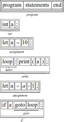
The Scanner will have to identify various language atoms and generate corresponding tokens, which is a one-to-one mapping. For example, the following atom identification should take place for our example simple program:
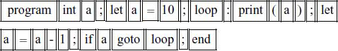
The corresponding token types are:
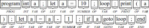
A token is a pair (type, value). For the example simple program given above, the token sequence generated by the Scanner is
 (265 0)  (268 0)  (258 0)   (259 59) (267 0)  (258 0)
 (259 61) (257 10) (259 59)  (258 1)  (259 58) (262 0) (259 40)
 (258 0)  (259 41) (259 59)  (267 0)  (258 0)  (259 61)
 (258 0)  (259 45) (257 1)   (259 59) (260 0)  (258 0)
 (261 0)  (258 1)  (259 59)  (266 0)
In our implementation, the token types have positive integer values greater than 256, to maintain compatibility with later discussion of yacc. The token type values are declared in the header file simple.h as:
 #define   BASE       256
 #define   NUMBER     BASE+1
 #define   VAR        BASE+2
 #define   OP	      BASE+3
 #define   IF	      BASE+4
 #define   GOTO       BASE+5
 #define   PRINT      BASE+6
 #define   READ       BASE+7
 #define   LABEL      BASE+8
 #define   PROG       BASE+9
 #define   END        BASE+10
 #define   LET        BASE+11
 #define   INT        BASE+12
 #define   MAT        BASE+13
 #define   UNDEF      0
The tokens are stored as pairs defined by a structure:
struct lexv {
  int type;
  union {
    Symbol *sym;
    int value;
  };
};
Note the union as the token value – for some token types, for example VAR, we will use its assigned address in the memory as the value. This address is represented by a pointer to a corresponding node in a symbol table, formed as a symbol list. The symbol nodes have a structure:
typedef struct Symbol
{
  char *name;
  short type;
  short addrs;
  struct Symbol *next;
} Symbol;
Some of the fields in such symbol nodes will be filled in by later phases of the compiler – the Scanner fills in only name, type and next.
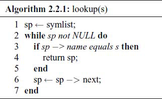
Whenever a variable is detected by the Scanner, a check is made by the function lookup ( ) to see if the identifier is present in the symbol list and if not present, the function install ( ) will insert it in the list. The algorithm for lookup ( ) is:
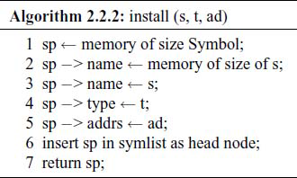
The algorithm for install ( ) is:
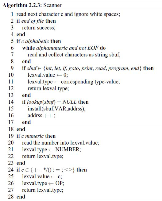
The Scanner algorithm is:
2.2.2 Parser
The job of a parser is to identify the syntactic entities in the source code, build and output the parse tree.
For the example simple program, the syntactic units should be identified as:
We have opted for implementing the parser for simple as a recursive-descent parser (RDP). This relatively simple parser implementation is possible if certain restrictions are put on the language and its grammar, see Chapter 4 for details.
The grammar with which the parser is concerned is given below:
program : PROG statements END
        ;
statements : statement
           | statements statement
           ;
statement : basic-statement ‘;’
          | label basic-statement ‘;’
          ;
basic-statement : assignment
                | var
                | if
                | goto
                | read
                | print
                ;
assignment : LET variable ‘=’ expr
             ;

var : INT variable
      ;
if : IF expr statement
     ;
goto : GOTO variable
       ;
read : read ‘(’ variable ‘)’
       ;
print : print ‘(’ number ‘)’
      | print ‘(’ variable ‘)’
      ;

expr : expr ‘+’ term
       | expr ‘-’ term
       | term
       ;

term : term ‘*’ factor
     | term ‘/’ factor
     | factor
     ;
factor : ‘(’ expr ‘)’
         | VAR
         | NUMBER
         ;

label : VAR ‘:’
      ;
Note that the identifiers written in all capitals are the token types passed on by the Scanner. The operation symbols like ‘+’ are token values for token type OP. The rest are the meta-variables of the grammar.
The basic idea in an RDP is that:
- For each NT and T symbols, there is a corresponding function which will try to check if the source code at a particular stage of processing can be generated using:
- if an NT – RHS of productions for that NT;
- if a T – it confirms that Terminal symbol.
For example, consider the productions for expr:
expr : expr ‘+’ term
       | expr ‘-’ term
       | term
       ;
The above portion of the grammar is in left-recursive form and needs to be converted to right-recursive or right-iterative form:
expr : term { ‘+’ term }
       | term { ‘-’ term }
       | term
       ;
where the curly brackets ‘{’ and ‘}’ enclose portions which may be repeated one or more times.
The corresponding algorithm pE ( ) looks like this:
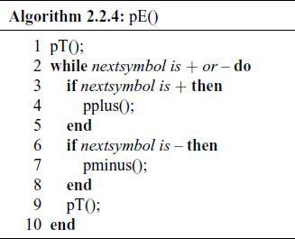
Here, pT ( ) is the algorithm, similar to the above, for recognizing all the productions from a term. The pplus ( ) algorithm is:
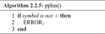
The algorithms for pminus ( ), and in fact all the Terminal symbols, are similar.
Notice the simplicity of algorithm – there is a one-to-one correspondence between the grammar production and the algorithm steps. We can write the algorithm almost by inspection.
The corresponding C language implementation should be looked up in the source file simple2.c available elsewhere.
Almost the complete parser is written this way, but two functions need special mention here. The parser gets its next token by calling the Scanner ( ). There is a bit of complication here – if you look at the algorithm, for example, for the pE ( ), you will notice that we are checking the nextsymbol in order to decide if we should go ahead and collect further terms and also if ‘+’ or ‘–’ is to be read and confirmed. We shall see in Chapter 4 why we need to do this look-ahead. We cannot get the nextsymbol by requesting Scanner ( ), as the meaning of a look-ahead is that we peep at the next symbol, but without processing it. Thus, we have a two-position “shifter” coded, which is initially empty (see Fig.2.2).
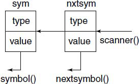
For each call to symbol ( ), a request goes to the Scanner to supply the next token and the shifter is shifted to the left. The very first call to symbol ( ) results in two calls to the Scanner. A call to nextsymbol ( ) does not result in a call to the Scanner, it simply allows a peep to the nxtsym in the shifter.
The algorithms described till now will just detect the syntax of various statements in the source code. They will decide if the statements are valid or not. Where is the parse tree expected to be generated as the output of the parser? In an RDP, it is “invisible”, rather it is in the call tree of various function that gets created as each statement is being parsed. For example, consider the following small program.
program
let a = 9;
end
The corresponding call sequence in the parser is
pPROG
  |
pSTS
  |
pST
  |
pLET -> pvar ->pasg ->pE
                      |
                      pT
                      |
                      pF
                      |
                      pnumber
 psemi <--------------+
pEND
What we are interested in is an Intermediate form of the code, from which we can easily generate the target code, the parse tree itself is not of direct interest. On the other hand, the intermediate form should be such that it facilitates the optimization of the target code and tends to give a clean separation of machine-independent and machine-dependent portions of the compiler, for the reasons suggested in Fig.1.13.
We define the intermediate form we plan to use in the next section.
2.2.3 Intermediate Form and Semantic Phase
There are several possible intermediate forms, as will be discussed in Chapter 8, some of which are tree data structure (Abstract Syntax Tree), a directed acyclic graph (DAG) and N-tuple, of which two-address code (TAC) is an instance. We use here the two-address code method.
The TAC or 3-tuple is a linear sequence or array of 3-component entries, each having a structure shown in Fig.2.3.
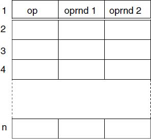
This array is called the matrix. The three components have the following significance and use:
op – the “operation” to be done
oprnd 1 – the first “operand”
oprnd 2 – the second “operand”
Each of these components is a token. An additional token type is now defined – MAT, which denotes result obtained when a specific entry is “executed”. The token value for MAT denotes the entry number.
Thus, it is seen that this form of code looks some what like machine code of some abstract machine. For our example simple program, the intermediate form output is given below:
0: (INT,0)	 (VAR,0) (,0)
1: (LET,0)	 (VAR,0) (NUMBER,10)
2: (LABEL,0)	 (VAR,1) (OP,58)
3: (PRINT,0)	 (VAR,0) (,0)
4: (OP,45)	 (VAR,0) (NUMBER,1)
5: (LET,0)	 (VAR,0) (MAT,4)
6: (IF,0)	 (VAR,0) (,0)
7: (GOTO,0)	 (VAR,1) (,0)
8: (FI,0)	 (,0)	 (,0)
9: (END,0)	 (,0)	 (,0)
The meaning of this sequence is:
entry 0 op = INT which denotes that an integer is being declared; oprnd1 = address assigned to variable ‘a’. oprnd2 is unused.
entry 1 op = LET which denotes that an assignment is to be made; oprnd1 is the address of ‘a’; oprnd2 is the RHS value to be assigned.
entry 2 op = LABEL: set a label on this entry, oprnd1 = label ‘loop’.
entry 3 op = PRINT: a value to be printed; oprnd1 = address of ‘a’.
entry 4 op = OP, value is ‘–’, i.e. minus operation; oprnd1 is ‘a’; oprnd2 is number 1. This will execute as a – 1 and the result will be known as MAT,4.
entry 5 op = LET: assignment to oprnd1 = ‘a’, value assigned is oprnd2 = MAT,4, i.e. result of the entry 4. Effectively, a = a – 1.
entry 6 op = IF: oprnd1 is ‘a’; if value of oprnd1 is non-zero, do the next entry and subsequent entries till op = FI.
entry 7 op = GOTO: oprnd1 is label ‘loop’.
entry 8 op = FI: end of “range” of the IF predicate.
entry 9 op = END: end of the program.
How does this intermediate code get generated? We can argue like this: the very fact that the RDP takes a recursive descent for a statement indicates that something is to be done first, before doing whatever is at hand. Thus, the code is generated and inserted in the matrix while the parser is ascending out of the descent. For details about the order of execution of statements within a recursive function, you may refer to the section on “Execution Trace and recursive functions”, under Section A.1.8.
Thus, the trick is to put all the code generation and insertion steps after a recursive call, to make it executed during the ascent.
For example, consider a statement
let a = b + c * d ;
The algorithm segment for a LET statement is:

The parser will detect an assignment statement (due to ‘let’), look for a variable, encounter ‘a’ and its token is assigned to t1. Then it looks for and confirms the ‘=‘ with pasg ( ). Then it invokes pE ( ), the function to recognize all the substrings which can get produced out of non-terminal expr. That function will parse the RHS expression and generate and insert in matrix whatever the 2-address code is needed to calculate the expression. The final result of the calculation will be represented by a particular matrix line, say n, and token (MAT, n) will be returned by pE ( ), which is assigned to t2. As the last step, an entry (t, t1, t2) will be inserted in the matrix, which specifies assignment (LET) to specified variable, the result of expression detected by pE ( ). Note very well that all the matrix entries needed to calculate the RHS expression are generated and inserted in the matrix, before the assignment operation entry is inserted.
The extended algorithm for pE ( ) is:
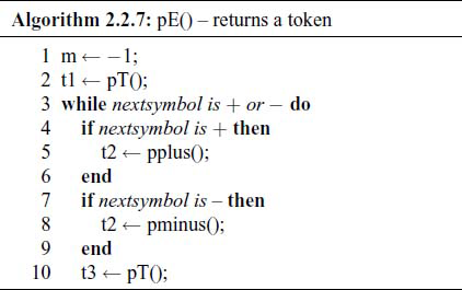
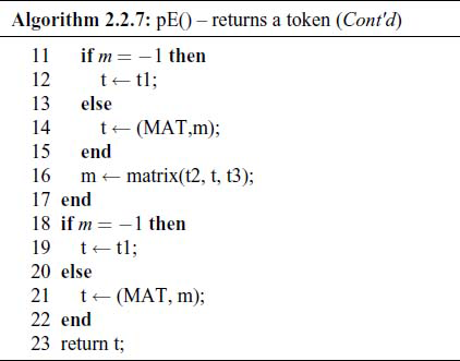
We have already encountered this algorithm above, but here we have added a few more steps to generate the 2-address code. The algorithm for pT ( ) is similar. The algorithm for pF ( ) is given as Algorithm 2.2.8.
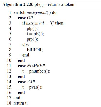
Note that pF ( ) itself does not insert any entries in the matrix. The 2-address code generated is:
0: (OP,42)   (VAR,2) (VAR,3)
1: (OP,43)   (VAR,1) (MAT,0)
2: (LET,0)   (VAR,0) (MAT,1)
The matrix line 0 specifies a ‘*’ operation on ‘c’ and ‘d’, line 1 specifies a ‘+’ operation on ‘b’ and result of line 0, and line 2 specifies ‘=’ operation on ‘a’ with result of line 1 as the RHS. You should trace through the algorithms for pE ( ), pT ( ) and pF ( ) and satisfy yourself that the above matrix will be obtained.
Now we discuss how the target language code, for our machine VM1, is generated.
2.2.4 Code Generation
Once we have the linear 2-address intermediate code, code generation for VM1 is comparatively straightforward. We have a separate program codegen.c for this operation. It accepts the output from parser-cum-semantic routines in simple2.c and generates the “machine language” code for VM1. Our test program source code is:
program
int a ;
let a = 10 ;
loop: print (a) ;
let a = a – 1 ;
if a goto loop ;
end
The Scanner-parser stages gave us an intermediate form output (in numeric form):
0  268  0  258  0  0	0
1  267  0  258  0  257  10
2  264  0  258  1  259  58
3  262  0  258  0  0	0
4  259  45 258  0  257  1
5  267  0  258  0  269  4
6  260  0  258  0  0	0
7  261  0  258  1  0	0
8  270  0  0    0  0    0
9  266  0  0    0  0    0
which is equivalent to intermediate code in alphabetic form:
0: (INT,0)	 (VAR,0)	 (,0)
1: (LET,0)	 (VAR,0)	 (NUMBER,10)
2: (LABEL,0)	 (VAR,1)	 (OP,58)
3: (PRINT,0)	 (VAR,0)	 (,0)
4: (OP,45)	 (VAR,0)	 (NUMBER,1)
5: (LET,0)	 (VAR,0)	 (MAT,4)
6: (IF,0)	 (VAR,0)	 (,0)
7: (GOTO,0)	 (VAR,1)	 (,0)
8: (FI,0)	 (,0)	 	 (,0)
9: (END,0)	 (,0)	 	 (,0)
When this intermediate code is given to codegen it produces the VM1 “machine code” output:
140 0 0 0 0 0      | place   for ‘a’
100 15 0 0 0 a     | LDI     A,   10
101 6 0 0 0 140    | ST      A,   a
102 5 0 0 0 140    | LD      A,   a
103 6 0 0 0 0      | ST      A,   0      (print)
104 5 0 0 0 140    | LD      A,   a
105 12 0 0 0 1     | SUBI    A,   1
106 6 0 0 0 204    | ST      A,   Temp4
107 5 0 0 0 204    | LD      A,   Temp4
108 6 0 0 0 140    | ST      A,   a
109 5 0 0 0 140    | LD      A,   a
10a b 0 0 0 0      | JN      A    ????   (Jump if -ve to ?)
10b 8 0 0 0 fff6   | JMP     -10         (jump to 102)
10a b 0 0 0    1   | JN      A    +1     (jump if -ve to 10C)
10c ff 0 0 0 100   | HLT                 (start address = 100)
For your reference, an “assembly language” comments are given, though not part of the code.
We have a number of comments on this code, but we postpone them till we first discuss how this code is generated.
The code generator uses a rather simple method to generate the VM1 code. Note that we have not used the full capabilities of VM1 while generating the code – only one machine register A is used as an accumulator, and various addressing modes like indexed, indirect, etc. are not used. As the simple language does not provide subroutines, we do not need to use the SP and BP registers either.
For each type of operation in the 2-address intermediate code, the code generator outputs one or two VM1 instructions. They are listed in Table 2.2.
Table 2.2 Mapping from Intermediate code to VM1 code
| Intermediate | VM1 machine code | codegen actions and remarks |
|---|---|---|
| INT opr1 | dataadrs,0,0,0,0,0 | loader will reserve and clear this location. |
| vartab[opr1]← dataadrs | ||
| dataadrs++ | ||
| LET opr1 opr2 | txtadrs, LD/LDI,0,0,0,opr2 | LD if opr2 is VAR or MAT |
| LDI if opr2 is NUMBER | ||
| opr2 = matstart + opr2 or datastart + opr2 | ||
| txtadrs++ | ||
| opr2 = matstart + opr2 or datastart + opr2 | ||
| txtadrs, ST,0,0,0,opr1 | opr1 = datastart + opr1 | |
| txtadrs++ | ||
| PRINT opr1 | txtadrs, LD/LDI,0,0,0,opr1 | LD if opr1 is VAR |
| LDI if opr1 is NUMBER | ||
| txtadrs++ | ||
| txtadrs, ST,0,0,0,0 | txtadrs++ | |
| READ opr1 | txtadrs, LD,0,0,0,0 | txtadrs++ |
| txtadrs, ST,0,0,0,opr1 | txtadrs++ | |
| OP,op opr1 | txtadrs, LD/LDI,0,0,0,opr1 | LD if opr1 is VAR or MAT |
| opr2 | LDI if opr1 is NUMBER | |
| opr1 = matstart + opr1 or datastart + opr1 | ||
| txtadrs++ | ||
| txtadrs, op,0,0,0,opr2 | op is ADD,SUB,MUL,DIV | |
| or their immd form if opr2 is NUMBER | ||
| opr2 = matstart + opr2 or datastart + opr2 | ||
| txtadrs++ | ||
| txtadrs, ST,0,0,0, matl | matl = matstart + lineno | |
| txtadrs++ | ||
| END | txtadrs, HLT,0,0,0,txtstart | |
| LABEL opr1 | vartab[opr1] = txtadrs | |
| IF opr1 | txtadrs, LD,0,0,0,opr1 | opr1 = matstart + opr1 or datastart + opr1 |
| txtadrs++; push(txtadrs) | ||
| txtadrs, JN,0,0,0,0 | the 0 address will be replaced | |
| txtadrs++ | ||
| GOTO opr1 | txtadrs, JMP,0,0,0, gotoadrs | opr1 = vartab[opr1] |
| gotoadrs = opr1 – txtadrs | ||
| txtadrs++ | ||
| FI | opr1, JN,0,0,0,gotoadrs | opr1 = pop() |
| gotoadrs = txtadrs-opr1–1 | ||
| replace JN instr as a JN “here” | ||
| we are overwriting |
Three VM1 memory address counters and some data areas are maintained by the codegen ( ):
txtadrs: Address where the next generated VM1 instruction will be positioned. This counter is incremented on each generated instruction.
dataadrs: Address where some data specified by int declarations are positioned. This counter is incremented on each generated data area allocation.
matadrs: Address where temporary locations, known as the MAT locations, used during the intermediate code generation, are located.
stack: where the jump address used to implement IF and GOTO are pushed and popped.
vartab: An address array where the assigned VM1 memory address of each of the variables is stored.
The LABEL, GOTO, IF and FI require a somewhat special treatment, because they can result in a forward jump in the target code. The forward jumps are managed through use of an address stack. The semantics of our if statement requires that if the value of the expression is non-negative, execute the sub-statement, otherwise go to the next statement. This means we have to insert a Jump-if-Negative instruction when an if is encountered. Unfortunately, we do not know the address to which this jump should take place, as the matching FI may be several instructions in the forward direction. We insert a zero address JN instruction and remember where it is positioned by pushing its address on a stack. Later, when an FI is encountered, we pop the stack, and replace the old JN instruction with a new one, with a proper address. As our loader for VM1 is a random address loader, this can be easily achieved.
The possibility of a forward LABEL is dealt with in a simple way. At the beginning of the codegen ( ), a scan of the intermediate code is performed, and when a LABEL is encountered we save the VM1 memory address where it occurred in the vartab. This is possible to do, as we know how many instructions are generated for each type of operation in the intermediate code. These lengths are stored in a data array instrlen. Later, when a GOTO is encountered with that identifier as the label, we simply generate a JMP instruction with that saved address. The jump addresses are adjusted with respect to the current instruction address, as required by the semantics of VM1.
The action of codegen for remaining intermediate code operations is rather straightforward one-to-one mapping and should be clear from Table 2.2.
2.2.5 Comments on the Compiled Code
The compiled code for the example program was executed on the VM1 simulator described in Section 2.3 and executed properly. If you compare the “machine code” given there with the compiled code given in Section 2.2.4, you will notice considerable differences, though both of them achieve exactly the same computation. The compiled code is almost double the size of a code written by an expert VM1 programmer.
The most noticeable difference is in the use of unnecessary Load and Store instructions. If a previous instruction has left a useful value in the A register, it is not necessary to load it again. Removal of such redundant instructions is a kind of optimization, which a good real-life compiler will definitely provide.
Also, the Jump instructions can be trimmed – instead of JN … JMP … sequence to encode if a goto loop; statement, we could have used a single JP instruction.
In the simple example that we took up as illustration, it is not very evident, but we could improve the compiled code by utilizing the additional machine registers available and avoid using the temporary memory locations to store values.
We shall discuss these matters in more details in later chapters on “Optimization”, Chapters 9 and 10.