
9.8 Machine-dependent Optimization
The naïve code generator that we have demonstrated several times does generate code which will execute (after assembly and linker steps) but the code quality is rather poor, in the following respect:
- Program size is big because the generated instruction sequences are quite long.
- Program execution time is long because there are redundant instructions and/or memory transfers.
- There is an inadequate use of CPU registers.
- The code generator does not make good use of the facilities of the machine, in the form of power of the instruction set.
An example: with the E compilation scheme, the statement:
total = total + count * count;
compiles to:
movl   total, %eax
pushl  %eax
movl   count, %eax
pushl  %eax
movl   count, %eax
popl   %ebx
imull  %ebx,  %eax
popl   %ebx
add    %ebx,  %eax
movl   %eax,  total
This translation has 10 instructions, 8 of which are accessing memory. Some of the memory accesses are unavoidable, but some of them seem avoidable if we use registers.
9.8.1 Register Allocation
Making Better Use of Registers
Up to now we have used only two registers in the generated code. Now let us take another extreme and imagine that we have as many registers as we need. We call them r(0), r(1), r(2), r(3), r(4), r(5), …. Can we generate a better code with all these registers available?
One trick is to store our stack of intermediate results in these registers and instead of using a stack pointer at run-time, we use our own stack pointer, sp. The compiler can keep track of where this stack pointer sp will be during compile-time. This arrangement leads us to another compilation scheme to generate code using our stack of registers.
Er[e](sp) generates code that will evaluate the expression e and leave the result in r(sp), without changing any of the registers below r(sp). For example,
Er[e1 + e2](sp) = Er[e1](sp)
                  Er[e2](sp + 1)
                  addl r(sp + 1), r(sp)
The scheme of arranging for intermediate values to be held in registers rather than memory locations is known as register allocation. That is how the name Er for the new compilation scheme has come about – E for expressions, r for register allocation. There are many different algorithms for register allocation. The approach we use here is one of the simplest, but not likely to be used in real compilers.
Some more examples are:
Er[n](sp)        =     movl $n, r(sp)
Er[v](sp)        =     movl v, r(sp)
Er[el && e2](sp) =     Er[e1](sp)
                       cmpl $1, r(sp)
                       jnz lab1
                       Er[e2](sp)
                 lab1: …

Er[v = e](sp)    =     Er[e](sp)
                       movl r(sp), v
Compiling Statements
The rules for compiling statements need to be modified for the register-based code. Note that the intermediate values are used only while evaluating an expression, and the stack is expected to return to its original state at the end of evaluation of the expression. We can thus assume the stack is empty when we need the value of an expression:
Sr[e]           =      Er[e](0)
Sr[while(e) s] =       jmp lab2
                 lab1: Sr[s]
                 lab2: Er[e](0)
                       cmpl $1, r(0)
                       jz lab1
Taking the example statement total = total + count * count:
Sr[total = total + count * count]
         = Er[total = total + count * count](0)

         = Er[total + count * count](0)
           movl r(0), total

         = Er[total](0)
           Er[count * count](1)
           addl r(1), r(0)
           movl r(0), total

         = movl total, r(0)
           Er[count * count](1)
           addl r(1), r(0)
           movl r(0), total

         = movl total, r(0)
           Er[count](1)
           Er[count](2)
           imull r(2), r(1)
           addl r(1), r(0)
           movl r(0), total

         = movl total, r(0)
           movl count, r(1)
           Er[count](2)
           imull r(2), r(1)
           addl r(1), r(0)
           movl r(0), total

         = movl total, r(0)
           movl count, r(1)
           movl count, r(2)
           imull r(2), r(1)
           addl r(1), r(0)
           movl r(0), total

         = movl total, %eax
           movl count, %ebx
           movl count, %ecx
           imull %ecx, %ebx
           addl %ebx, %eax
           movl %eax, total
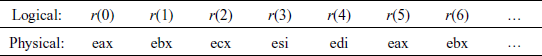
In the last step, we replace the assumed registers with real registers of the processor. Now we are making better use of registers. Any code to implement this particular statement would have to do two loads, one add, one multiply and one store. So now we are just one instruction away from optimal.
To make this compilation scheme work properly, we need to do a stack simulation, by adding a compile-time parameter to tell us what the stack size will be at the corresponding point at run-time.
Suppose we also try to track the run-time contents of the stack at compile-time. We shall write a stack in the form [e0, …, en] where e0, …, en are expressions, or a special symbol ‘?’ which represents unknown.
Going back to our example code segment:
Sc[total = total + count * count]
         = Ec[total = total + count * count] []

         = Ec[total + count * count][]
           movl r(0), total

         = Ec[total] []
           Ec[count * count] []
           addl r(1), r(0)
           movl r(0), total

         = movl total, r(0)
           Ec[count * count] [total]
           addl r(1), r(0)
           movl r(0), total

         = movl total, r(0)
           Ec[count][total]
           Ec[count][total]
           imull r(2), r(1)
           addl r(1), r(0)
           movl r(0), total

         = movl total, r(0)
           movl count, r(1)
           Ec[count] [total, count]  The stack description here shows that
                                     count  has  already  been  loaded  into
                                     register r(1) so we do not need to
           movl r(0), total
                                     load it again now
           imull r(2), r(1)
           addl r(1), r(0)
           movl r(0), total
Now we note that:
Ec[v][e0, …, en]
              = movl r(i), r(n + 1)   if ei = v
                movl v, r(n + 1)      otherwise
This gives us:
Sc[total = total + count * count]
  = movl total, r(0)
    movl count, r(1)
    movl r(1), r(2)
    imull r(2), r(1)
    addl r(1), r(0)
    movl r(0), total
This is one more instruction than what we needed, but we have eliminated the duplicated memory access. The redundant instruction too can be eliminated using an optimization method known as copy propagation.
Some instruction sequences can invalidate the cache entries. For example, consider:
(total + (total = 2) + total)
Naïvely applying the previous compilation scheme would give us a code like the following:
movl total, r(0)
movl $2, r(1)
movl r(1), total   Total has been changed, so we cannot use r(0) as a shortcut
                   to total anymore. And, in fact, we are overwriting r(0)
addl r(1), r(0)    In fact, we are overwriting r(0) here with another value
                   anyway.
movl r(0), r(1)
addl r(1), r(0)    So using the value in r(0) here is definitely a mistake!
To avoid such problems, we have to keep the cache accurate, by tracking the cache more carefully.
movl total, r(0)[total]
movl $2, r(1)[total, 2]
movl r(1), total[?, total = 2]   The  cache  has  two  different  symbolic
                                 representations of the value in r(1) at
                                 this point
addl r(1), r(0)[?, total = 2]    But the original value for total has been
                                 overwritten.
movl r(1), r(1)
addl r(1), r(0)[?]
This shows that we can determine considerable information about the run-time behaviour of a program by using symbolic data at compile-time. One has to be careful about subtle pitfalls and oversights. This is an area where formal methods can help.
In the real world, no processor has infinitely many registers built into it. An x86 series of processor has:
Accumulator eax
Base ebx
Count ecx
Data edx – cannot be used as a general register, used in mult and div instruction as extension of eax.
Source index esi
Destination index esi
Base pointer ebp – cannot be used as a general register, used as stack-frame base pointer.
Stack pointer esp – cannot be used as a general register, used as run-time stack pointer.
Instruction pointer eip – cannot be used as a general register, hardware instruction pointer.
Flags eflag – cannot be used as a general register, hardware flags.
After we have eliminated special purpose registers, an x86 has only five general-purpose registers available.
Register Pressure
The number of registers that we need for a given computation is sometimes described as register pressure. High register pressure occurs most frequently when we are compiling for processors with very few registers. We can deal with register pressure by using registers more carefully and using register spilling when all else fails.
To illustrate the first solution, i.e. “Use Registers Carefully”, let us take our previous example;
S[total = total + count * count]
   = movl  total, r(0)             use register r(0) to hold the value
     movl  count, r(1)             of total we do not actually need the
     imull r(1),  r(1)             value of total until after we have
     addl  r(1),  r(0)             calculated count * count. We may delay
     movl  r(0),  total            the load of total
We rewrite the code as:
S[total = total + count * count]
   = movl count, r(0)
     imull r(0), r(0)
     movl total, r(1)
     addl r(1), r(0)
     movl  r(0),  total
This has not changed the number of registers that we need, but it has shown a possibility for better code. Instead of loading total into r(1), we can add it directly to r(0).
S[total = total + count * count]
   = movl  count, r(0)
     imull r(0),  r(0)
     addl  total, r(0)
     movl  r(0),  total
Now we are using only one register and also fewer instructions. These improvements would be particularly important if we were dealing with a subexpression of some larger statements where more registers were needed.
Minimizing Depth
It can be proved that we use fewest registers if we evaluate the subexpression with greatest depth first. The syntax tree for our example is:

and the corresponding depth values are:

Note that application of the above rule will force evaluation of the RHS subtree, c * c first and then addition to t. If instead of addition we had subtraction and we evaluate the arguments of a subtraction in the reverse order, then we will have to use an xchgl instruction before subl. If we evaluate the arguments of an addition in the reverse order, then an addl by itself will be acceptable, as addition operation is commutative.
While applying the above rule we have to be careful about the side effects. If the arguments of an operator might have side effects, then we may not be able to change the order. For example, suppose that some function f(x) prints the value of x on the console. If we are generating code for the expression f(3) + (1 + f(2)), value 2 will be printed before 3.
Some languages specify an explicit order of evaluation. Others leave the choice unspecified to give the implementer more flexibility.
Register Spilling
The term register spilling refers to the process of moving temporary values from registers into the run-time stack. Conceptually, we use our finite set of registers, together with the memory stack, to simulate our infinite family of registers r(i):
In practice, we modify our compilation schemes to use spilling to reserve space when they need a new register. For example,
Er[e1 + e2](sp) = Er[e1](sp)
                  spill(sp + 1)
                  Er[e2](sp + 1)
                  addl r(sp + 1),r(sp)
                  unspill(sp + 1)
where
spill(sp)    = pushl r(sp), if sp >= 5,
             = null,        otherwise
unspill(sp)  = popl r(sp),  if sp >= 5,
             = null,        otherwise
With only two registers, our example code requires:
S[total = total  + count  * count]
        = movl    total,  r(0)
          movl    count,  r(1)
          pushl   r(2)
          movl    count,  r(2)
          imull   r(2),   r(1)
          popl    r(2)
          addl    r(1),   r(0)
          movl    r(0),   total
If we had just two registers, and had not made the other improvements, this is the code we would end up with. Note that r(0) = r(2) = eax, and r(1) = ebx.
The moral is: use registers when we can, and use spilling when we have to.
Making Use of Context
To get better code, we add information about the context in which the expression appears to our compilation scheme. Without context information, a compilation scheme must work in all places where that expression could appear. With context information, the compilation scheme needs only to produce code that works in the specified context.
Recurring Patterns
Recall the compilation rules for logical-AND and while-loop:
Er[e1 && e2](sp) =     Er[e1](sp)      |
                       cmpl $1, r(sp)  |*
                       jnz lab1        |
                       Er[e2](sp)
                 lab1: …
S[while(e) s]   =      jmp lab2
                 lab1: S[s]
                 lab2:
                       Er[e](0)        |
                       cmpl $1, r(0)   |*
                       jz lab1         |
The blocks of code marked ‘*’ on the RHS use the result of a Boolean expression to make a jump; they do not actually need the result itself. We give the two patterns a name
branchTrue[e](sp,label)  = Er[e](sp)
                           cmpl $1, r(sp)
                           jz label
branchFalse[e](sp,label) = Er[e](sp)
                           cmpl $1, r(sp)
                           jnz label
Note that we have added the label, an extra context, as an additional argument. We have now the new schemes by abstracting details from the compilation schemes. Now we can rewrite the compilation schemes to utilize them:
Er[e1 && e2](sp) =       branchFalse[e1](sp,label)
                         Er[e2](sp)
                 label:  …
S[while(e) s]   =        jmp label2
                 label1: S[s]
                 label2: branchTrue[e](0,label1)
We can produce special compilation rules for some conditional jump constructs:
branchTrue[true](sp,label)  = jmp label

branchTrue[false](sp,label) = null

branchTrue [e1 || e2](sp,label) = branchTrue[e1](sp,label)
                                  branchTrue[e2](sp,label)

branchTrue [el && e2](sp,label) = branchFalse[e1](sp,label1)
                                  branchTrue [e2](sp,label)
                          label1:
We do get benefits from this improved code. For example, with the original compilation schemes, we get:
S[while(el && e2) s]   =     jmp label2
                     label1: S[s]
                     label2: Er[e1](0)
                             cmpl $1, r(0)
                             jnz label3
                             Er[e2](0)
                             cmpl $1, r(0)
                             jz label1
                     label3:
With the modified compilation schemes, we get:
S[while(el && e2) s]   =     jmp label2
                     label1: Srs[s]
                     label2: branchFalse[e1](0,label3)
                             branchTrue[e2](0,label1)
                     label3:
If either e1 or e2 fits the special cases that we have defined for branchTrue or branchFalse, then we will get even better code.
There are a few more compilation schemes which are of interest. The increment operator, ++, in Java, C and C++ can be implemented using:
var++ = movl var,%eax        ++var = incl var
        incl var                     movl var,%eax
If var++ or ++var appears in an expression, then the final value in eax is important. If either appears as a statement, then the final value is not important, and we can compile either as just incl var. We can distinguish the different contexts by matching for ++ expressions both in the S and the E schemes.
Java, C and C++ provide two ways of escaping from a loop:
while(…){           while(…){
      …                   …
   }                       cont:
                      }
                      past:
A break statement in the left loop is equivalent to goto past in the right one. A continue statement in the left loop is equivalent to goto cont in the right one. The innermost cont and past labels must be passed as context parameters to the S scheme, in order to support breaking and continuation of loops.
We have seen that with careful selection of compilation schemes, we can produce good quality assembly language code, directly from the verified representation of a program. Register allocation makes a big difference in performance and code size. Register spilling is used to cope with limited numbers of registers. Instruction scheduling can make a difference to execution time on modern machines. The more information that we have about the context of a program segment, the better is the code that we can generate for it.
9.8.2 Instruction Rescheduling: Use of Parallelism in Instruction Execution
An important aspect of modern processors’ architecture which concerns machine-dependent optimization is Instruction Pipelining. This is a kind of parallel operation within a single processor. However, to derive maximum possible benefits from the hardware scheme, the instructions in the target code are to be rescheduled, i.e. their order of execution is changed, at the same time taking care to preserve the semantics of the original code.
Instruction Pipelining
The processor has several steps (or stages) in treating each instruction. The stages vary from one processor to another, but it can generally be broken down into following stages:
Fetch stage: In this stage, the processor fetches the instruction from the memory (or the cache).
Decode stage: In this stage, the processor tries to figure out the meaning of the instruction. Remember that the instruction is in the form of machine code.
Execute stage: After figuring out the meaning, the processor executes the instruction. Here, the processor also fetches any data in memory if needed. In that case, the execute stage is considered to be divided in two stages – data fetch and execute.
Write-back stage: If there are results need to be stored back to the memory, the processor dispatches them.
Each of these stages can actually be expanded into several stages. The old Pentium, for example expand the execution stage into two: one stage is to fetch any data from memory if needed, the other is to actually execute it. Also, in the Pentium, after the write-back stage, we have “error reporting” stage which is, obviously, to report errors if any. Even Pentium 4 has 20 stages.
Obviously, these stages are arranged into a single sequential pipeline so that the instruction enters from the first stage, sequentially to the end as shown in Fig. 9.10.
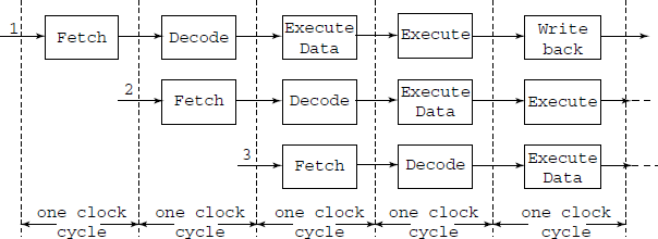
Fig. 9.10 Instruction execution pipeline. At a time more than one instruction are in various stages of their execution. The processor starts Fetching the next instruction as soon as the previous one enters its Decode stage. This is anticipatory fetching or pre-fetch. With such pre-fetch, the L-1 and L-2 cache’ get filled up. A problem arises when a conditional jump, or even a simple jump, invalidates the pre-fetched instructions. Then the cache’ has to be filled ab initio
Staging the instruction process has a great advantage. Suppose you have instruction 1 to n to be executed sequentially. At clock 1, instruction 1 enters the first stage. At clock 2, instruction 1 enters the second stage. Since at clock 2, the first stage is empty, we can feed in instruction 2. At clock 3, instruction 1 is at stage 3, and instruction 2 is at stage 2, so we can put in instruction 3 into stage 1, and so on.
The effect of all these is this: if we have four stages of processing, it is like processing 4 instructions at the same time (but in different stages). So the net effect is four times the “normal” performance. Thus pipelining certainly boosts up performance.
However, there is a catch: if we have conditional jumps then the performance boost may not be as expected. If instruction number 3 is being executed, thus in stage 3 in Fig. 9.10, the instructions in stages 1 and 2 must be cancelled if the prediction is wrong. What is prediction? The very fact that the jump instruction is in stage 3 means that the processor assumes that the jump, if at all taking place, will be such that the instructions which have entered stages 1 and 2 will in fact be executed next.
Today's computers have more than one pipeline. This is referred as multi-pipeline processor. The old Pentium had two pipelines, so it was like having two separate processors working simultaneously. If we have two pipeline, the processor can execute two instructions in parallel. If each pipeline has 5 stages, we effectively pump up the performance up to 10 times. Running two or more instructions in parallel needs a precaution: These instructions must be independent of each other in order to be able to be executed in parallel. For example,
mov bx, ax
mov ex, bx
These instructions cannot be run in parallel, because the second instruction needs the outcome of the first instruction, i.e. the value of BX is determined by the result of the first instruction. Look at the next example:
mov bx, ax
mov ex, ax
This program segment can be run in parallel because now both of them only depend on AX, which is assumed already set previously. We know that both segments mean the same thing, but the second example is faster because it can run in parallel. Therefore, the instruction reordering can make the difference because of multi-pipelining.
The conclusion is: if you want to speed up your code, it is worth reordering the instructions so that many of them can be run in parallel.