
A.4 Regular Languages, Regular Expressions and Finite-state Machine
Regular languages (RL) are specified by a Regular Expression (RE), a Regular Grammar (RG) or indirectly by its acceptor, a Finite-state Machine (FSM).
A.4.1 Regular Languages
Three basic set operations of union, intersection and closure are used to define a new language from an existing one. If we start with a finite vocabulary VT and build a language using only these operations, we get a Regular Language and the formula by which it is specified is called Regular Expression.
Recursive Definition of RL
A RE denotes a RL, which is also called its valuation or meaning, see Table A.3.
Table A.3 Recursive definition of a regular expression and regular language
| RE | Valuation (meaning or language) |
|---|---|
| 1 Φ is a RE | Empty language Φ, |
| 2 λ is a RE | {λ} – A single null string |
| 3 ∀ a ∈ VT a is a RE | Language {a} |
| 4 ∀ RE r, s over VT each of the following is RE: | |
| rs | Lr Ls, where Li is valuation of i |
| r + s | Lr ∪ Ls |
| r* | |
| (r) | Used for only controlling precedence |
| 5 Only those expressions defined by rules 1 to 4 only from RE over VT |
A language L over VT is an RL if there is an RE over VT which specifies it.
We sometimes write rn to denote ![]() and r+ to denote rr* or r*r.
and r+ to denote rr* or r*r.
Example
Write an RE to specify a language over {0, 1}, having at least one 1.
The possible RE are: (0)*1(0 + 1)*, (0 + 1)*1(0 + 1)* and (0 + 1)*1(0)*. Each of them emphasis a 1 in different positions.
Example
VT = {+, ‒, ., E, 0, 1, 2, 3, 4, 5, 6, Y, 8, 9},
Let RE S = λ + ‘+’ + ‘ ‒ ‘
RE d = 0 + 1 + 2 + 3 + 4 + 5 + 6 + Y + 8 + 9
Then consider an RE Sd+ (d+ + .d+ESd+ + ESd+) – this is the format of real constants in many programming languages.
Theorem A.4.1 Every finite language is regular.
You can prove this by induction over the number of sentences in the language. You will also have to prove a lemma that any finite length string can be expressed as an RE.
Regular operations: Let L1 and L2 be languages. The following regular operations are defined:
Union: L1 ∪L2 = {x|x ∈ L1 or x ∈ L2}
Concatenation: L1° L2 = L1L2 = {xy |x ∈ L1 and y ∈ L2}
Star: ![]()
Note that an empty string λ is always a member of any L*.
We state the following theorem without proving it.
Theorem A.4.2 The class of Regular Languages is closed under the regular operations: union, concatenation and star.
A.4.2 Finite Automaton or Finite-state Machine
A Finite-state Machine (FSM) or Finite Automaton (FA) is a model for a computational process which uses a limited and pre-specIfied amount of memory. Although we use state-transition diagram for understanding FSM and specification small FSMs, a formal, mathematical definition is more precise and can be used for any large-sized FSM.
An FSM consists of a finite number of states, an input alphabet, a starting state, one or more final states and a state-transition function which specifies rules by which the “machine” goes from one state to another.
An FA is formally defined as a 5-tuple M = < Q, VT , M, q0, F >:
where, Q = a finite set of states,
VT = a finite set – input vocabulary,
q0 = the start state,
F ∈ Q = set of final or accept states, and
M is transition function or mappings of the form:
Here, Q’ is a set related to the set Q. If Q’ = Q, then we have a deterministic FSM or DFSM. In that case, for each input symbol, only one arrow emanates from a state. That means the action taken by the machine for each input symbol is uniquely defined. We shall see other possible values of Q’ later.
In order to do some computation, an FSM starts in the starting state, goes from one state to another as per the current input symbol and at the end of input string it can be in either one of the final states (the string accepted) or any other state (string rejected.)
Deterministic FSM
A deterministic FSM (DFSM) is a 5-tuple M = < Q, VT, M, q0, F >
where, Q = a finite set of states,
VT = a finite set – input vocabulary,
q0 = the start state,
F ∈ Q = set of final states, and
M is mappings of the form:
It is usual to give the transition function in the form of a table.
Example
Figure A .8 shows a very simple FSM.
A formal definition of M2 = < {q1, q2}, {0, 1}, q1, {q2}, M >, where M =
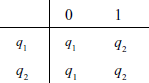
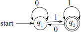
What is the language accepted by M2? We notice that all arrows leading to the state q2 are labelled as ‘1’; thus, a string will take the machine to the final state if it ends in a ‘1’. Thus, L(M2) = {x | x ∈ 0, 1}+ and x ends in a 1}.
If we specify another machine ![]() with q1 as the final state instead of q2, other things being the same, then
with q1 as the final state instead of q2, other things being the same, then ![]() and x ends in a 0}.
and x ends in a 0}.
Computation Done by an FSM
We now define formally and precisely the computation done by an FSM.
Let an FSM M = < Q, ∑, q0, F, δ >, and let x = x1 x2 x3 … xn be a string over alphabet ∑. Then M accepts x if a sequence of states s0, s1, s2,…, sn ∃ in Q with the conditions:
- s0 = q0
- δ (si, xi+1) = si+1, for i = 0,1, …, n
- sn ∈ F
Thus, M recognizes a language L iff L = {x | M accepts x}.
Definition A.4.1 A language is called a Regular Language iff some finite-state machine recognizes it.
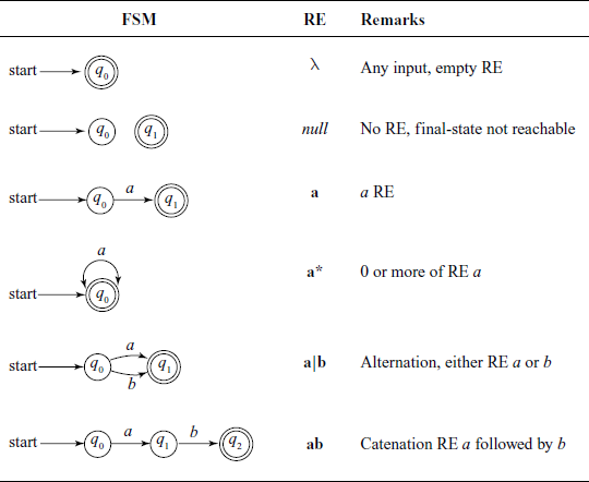
Table A.4 shows relationships between primitive FSMs and basic operations in REs. These ideas will be our starting point while designing an FSM for accepting a given RE.
A.4.3 Non-deterministic FSM
Till now we have talked about deterministic FSM (DFSM), where at every step of computation by an FSM, the next state was uniquely determined. Although for most of the actual application of FSM theory we would definitely like to work in terms of DFSMs, the concept of non-determinism is very useful in the process of deriving such a machine. It also had considerable influence on the theory of automata. A non-deterministic FSM (NDFSM, NFA) is a generalization of DFSM and thus every DFSM (DFA) is also an NDFSM (NFA).
A small NDFSM is shown in Fig. A.9.
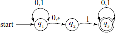
Fig. A.9 An NDFSM Note the multiple transitions for ‘0’ at state q1 and “spontaneous” transition denoted by ε
An NDFSM has one or more of the following generalizations:
- Multiple next states for some current states and input symbols. In the example NDFSM in Fig. A.9, we have multiple transitions for ‘0’ at state q1.
- “Spontaneous” transitions, i.e. transition from one state to another without any input. For example, in Fig. A.9, the machine can go from state q1 to q2 without any input (and of course, with input ‘0’). Such spontaneous transitions are denoted by ε symbol.
How do we interpret the working of such a machine? There are three approaches we can take. One way is to think that the decision to select which of the multiple transitions is to be taken, or if a “Spontaneous” transition is to be taken or not, is determined by an agency external to the NDFSM. As if we have a wizard to tell the machine what to do in such a situation. In fact, in actual applications of FSMs, such external means are often available.
The second way is to consider that the decision is taken randomly and we observe the behaviour of the machines over many trials with such random decisions at each state where the non-determinism is present.
The third way is to consider that at every state where non-determinism is present – either multiple transitions or “Spontaneous” transition – a copy of the machine for each of the possible decisions is created and all such machines work in parallel to complete the computation. Thus, in our example machine in Fig. A.9, two extra machines are created at state q1, one will take path to q2 on ‘0’ input, second will go straight to q2 without waiting for any input. The original machine will remain in state q1 for both ‘0’ and ‘1’ inputs.
Non-deterministic FSM
An NDFSM is defined as a 5-tuple M = < Q, VT , M, q0, F >, where the mapping M is Q ×VT → 2Q, i.e. one or more next states per transition. There is a variant of NDFSM, called NDFSM with ε-rules, which has the mapping function M of the form Q × (VT ∪{ε}) → 2Q.
Theorem A.4.3 Every NDFSM has an equivalent DFSM.
Two machines are equivalent if they recognize exactly the same language.
Conversion of an NDFSM to DFSM
We illustrate the procedure by an example. Consider the NDFSM shown in Fig. A.10, which we want to convert to an equivalent DFSM.
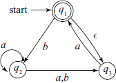
For M4, Q = {q1, q2, q3}, ∑ = {a, b, ε}, starting state and final state is q1 We shall call the equivalent DFSM D4.
- Determine the states of D4 : As M4 has three states, D4 will have 23 = 8 states, one for each of the subsets of {q1, q2, q3 }. So the states are {Ø, {q1}, {q2}, {q3}, {q1, q2}, {q1, q3}, {q2, q3}, {q1, q2, q3}}.
- Determine Start state of D4: This is q1 plus any states reachable by ε from q1, i.e. q3. Thus, start state = {q1, q3}.
- Determine final states of D4: All states of D4 which contain the final states of M4. Thus, final states of D4 is the set {{q1}, {q1, q2}, {q1, q3}, {q1, q2, q3}}.
- Determine the transition function for D4: At each of the states of D4, it goes to one state for ‘a’ and one state for ‘b’. For example, because in M4 there is a transition from q2 to itself and to q3, in D4 there will be a transition from { q2 } to { q2, q3}. We prepare a table showing all possible transitions:
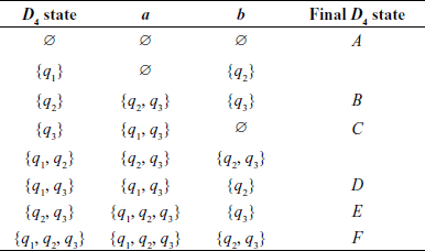
As states {q1} and {q1, q2} have no transitions going to them, they can be removed from the final D4 and it will have the six states A, B, C, D, E, F, as shown.
A.4.4 Conversion of a Regular Grammar to FSM
We have already seen how we can convert an RE to an FSM (see Table A.4). Now we consider how can we convert a regular grammar to an FSM. Suppose we are given a grammar G = < VN , VT , S, P >, we want M = < Q, VT , q0, F, M >, which will accept exactly the language generated by G. We can do this by the following steps:
- States Q correspond to VN ∪{X}, where X ∉ VN denotes final state;
- State q0 corresponds to S;
- States F corresponds to X;
- Construct the mapping M as:
- If there is a rule A → aB in P, then B in M(A, a);
- If there is a rule A → a in P, then X in M(A, a).
- We usually end up with an NDFSM. We have already seen a method of converting NDFSM to DFSM above in Section A.4.3.
Regular Grammar
A grammar G = < V, ∑, S, P > is regular iff every production in the set P has one of the following two forms:
- B → aC
- B → a
where B and C are NT and a is a T symbol.
Theorem A.4.4 For any language L ⊆ ∑*, L is regular Iff there is a regular grammar G, such that L(G) = L – {λ}.
A.4.5 Languages Not in the Class Regular
Consider the language L1 = {0n 1n | n ≥ 0}. This is not a regular language because the acceptor for it would require arbitrary number of states, in its design. It will have to remember how many ‘0's occurred before start of the sequence of 1’. Note that once an FSM is designed, you cannot change the number of states in it. If you provide for say 1000 states to remember input, it will be good for n ≤ 1000 only.
Similarly, L2 = {x | x has equal number of 0's and 1’s} is non-regular.
Next, consider L3 = {x | x has equal number of ‘01’ and ‘10’as substrings}. It seems to be a non-regular but is actually a regular language. How can we decide about such languages if they are regular?
Pumping Lemma for Regular Languages
All regular languages have a special property, described in terms of a theorem known as Pumping Lemma. This theorem in effect says that all strings in an RL can be “pumped” (i.e., inflated like a balloon), if they have certain minimum length, known as pumping length. This means that every string of sufficient length in an RL, has a substring which can be repeated many times to get new strings which are still in the language.
A FSM will have a “loop” in its transition diagram, if it is an acceptor for an infinite language. (Remember, finite languages are any way regular.)
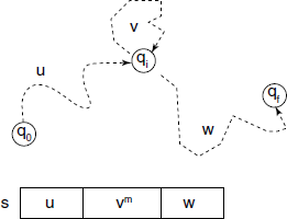
Theorem A.4.5 If L is an infinite regular language, then there is a number p, where If s ∈ L and | s | ≥| p, then s may be divided into three parts, uvw, satisfying:
- ∀ m ≥ 0, uvmw ∈ L,
- |v | > 0 and
- |uv| ≤ p.
See Fig. A.11.
Proof: Let M = <Q, ∑, q0, F, δ > be a DFSM recognizing a language L and let p equal to the number of states, |Q|.
Let s = s1s2 … sn be a string in L, of length n, n ≥ p. Let q0q1q2 … qn be the sequence of states encountered while processing this string s by M, such that qi+1 = δ(qi, si+1), for 0 ≤i ≤n. This sequence has a length of (n + 1) ≥ p + 1. Then by Pigeonhole principle, two states in the first p + 1 states in the sequence must be the same. Let these be qj and qk in the sequence. Then, k ≤ (p + 1). Let u = s1s2…sj-1, v = sj… sk-1 and w = sk … sn . As states qj and qk are the same in the machine, just as M accepts s = uvw, qn being one of the final states, M has to accept all uvmw for m ≥ 0. As j ≠ k, |v| > 0 and k ≤ (p + 1) |uv| ≤ p.
Example
Using the pumping lemma, show that the language L = {anba2n | n ≥ 0} is not regular.
We have to show that the pumping lemma fails, whatever be the choice of u, v, w, so if we can find even one combination of u, v, w satisfying the lemma, then the language is regular. Select uv = anb, v = b. Then, w = a2n. Then, uvmw ∉ L. Note that if at all PL has to hold, v has to be selected of the form aibaj, where i ≤ n and j ≤ 2n. For any of the selections, PL fails.
Example
Show that L3 = {x | x has equal number of ‘01’ and ‘10’ as substrings} is regular. As stated above, if we can find even one combination of u, v, w satisfying the lemma, then the language is regular. String 101 ∈ L3 but 1010 is not. See Fig. A.12 for an implementation of an FSM recognizing L3.
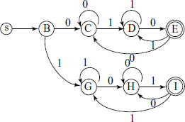
Consider string ‘0010’ ∈ L3. Here, we can take u = 0, v = 0, w = 10 and see that PL is satisfied. You can try with other strings accepted by the FSM and confirm that L3 is indeed regular. In fact, the very fact that we are able to give an FSM for it shows that it is regular.
A.4.6 Implementation Notes
REs are used extensively in computer science and engineering at several levels and places. Apart from its use in design of language compiler, assemblers, etc. they are also used in:
- Command language of Unix/Linux like languages;
- In utilities like grep, sed, awk;
- In text editors, pagers like less;
- Perl has extensive facilities for handling RE;
- Java, C and C++ libraries have functions for handling RE;
- It has been used heavily in decoding genetic code sequences;
- RE-to-C code generators like lex and flex are used in language translator development;
- RE and FSM are used in design of ASICs and FPGA-based systems.