

Rotoscoping is the process of drawing a matte frame by frame over live action footage. Starting around the year 50 B.C. (Before Computers) the technique back then was to rear project a frame of film onto a sheet of frosted glass, and then trace around the target object. The process got its name from the machine used to do the work, called a rotoscope. Things have improved somewhat since then, and today we use computers to draw shapes using the splines we saw in Chapter 5. The difference between drawing a single shape and rotoscoping is the addition of animation. Rotoscoping entails drawing a series of shapes that follow the target object through a sequence of frames.
Rotoscoping is extremely pervasive in the world of digital compositing and is used in a great many visual effects shots. It is also labor intensive because it can take a great deal of time to carefully draw moving shapes around a moving target frame by frame. It is often an entry-level position in the trade and many a digital compositor has started out as a roto artist. There are some that find rotoscoping rewarding and elect to become roto kings (or queens) in their own right. A talented roto artist is always a valued member of the visual effects team.
In this chapter we will see how rotoscoping works and develop an understanding of the entire process. We will see how the spline-based shapes are controlled frame by frame to create outlines that exactly match the edges of the target object as well as how shapes can be grouped into hierarchies to improve productivity and the quality of the animation. The sections on interpolation and keyframing describe how to get the computer to do more of the work for you, and then finally the solutions to the classic problems of motion blur and semi-transparency are revealed.
6.1 ABOUT ROTOSCOPING
Today, rotoscoping means drawing an animated spline-based shape over a series of digitized film (or video) frames. The computer then renders the shape frame by frame as a black and white matte that is used for compositing or to isolate the target object for some special treatment such as color correction.
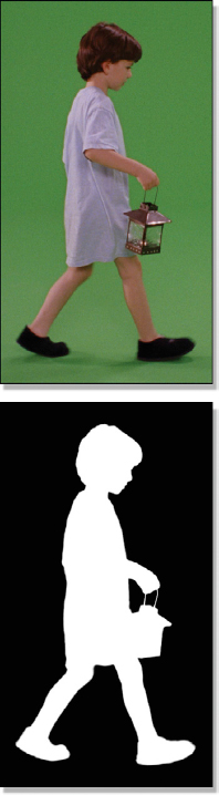
Figure 6-1 Frame 1 with roto
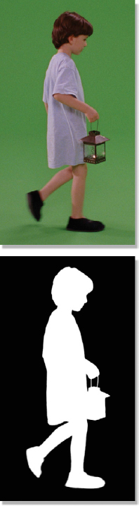
Figure 6-2 Frame 2 with roto

Figure 6-3 Frame 3 with roto
Figure 6-1 through Figure 6-3 illustrate three frames out of a moving sequence for a greenscreen shot that was rotoscoped. Not only does the target object (the boy) move, but he also changes shape as his feet move; his hand and lantern swing; and his head bobs while he walks. What makes it a “roto” (rotoscope) is that the outline of the shape needs to change every frame, so it must be animated.
(Download the folder at www.compositingVFX.com/CH06/Figure 6-1 and try your hand at rotoscoping the boy.)
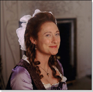
Figure 6-4 Original background
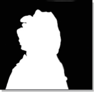
Figure 6-5 Roto matte
Figure 6-6 New background
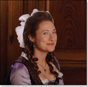
Figure 6-7 Composited
The virtue of roto is that it can be used to create a matte for any arbitrary object on any arbitrary background. It need not be shot on bluescreen. In fact, roto is the last line of defense for poorly shot bluescreens where a good matte cannot be created with a keyer. Compositing a character that was shot on an “uncontrolled” background is illustrated here starting with Figure 6-4. The bonny lass was shot on location with the original background. A roto was drawn (Figure 6-5) and used to composite the woman over a completely new background (Figure 6-7). No bluescreen required.
There are three main downsides to roto. First, it is labor intensive. It can take hours to roto a simple shot like the one illustrated in Figure 6-4, even assuming it is a short shot. More complex rotos and longer shots can take days, even weeks. This is hard on both schedules and budgets. The second downside to roto is that it can be difficult to get a high-quality, convincing matte with a stable outline. If the roto artist is not careful, the edges of the roto can wobble in and out in a most unnatural, eye-catching way. The third issue is that rotos do not capture the subtle edge and transparency nuances that a well-done bluescreen shot does using a fine digital keyer. If the target object has a lot of very fine edge detail, like a frizzy head of hair, the task can be downright hopeless.
6.2 SPLINES
In Chapter 5 we first met the spline during the discussion of shapes. We saw how a spline was a series of curved lines connected by control points that could be used to adjust the curvature of those lines. We also used the metaphor of a piano wire to describe the stiffness and smooth curvature of the spline. Here we will take a closer look at those splines and how they are used to create outlines that can fit any curved surface. We will also push the piano wire metaphor to the breaking point.
A spline is a mathematically generated line whose shape is controlled by adjustable control points. While there are a variety of mathematical equations that have been devised that will draw slightly different kinds of splines, they all work in the same general way. Figure 6-8 reviews the key components of a spline that we saw in Chapter 5—the control point, the resulting spline line, and the handles that are used to adjust its shape. In Figure 6-8 the slope of the spline at the control point is being adjusted by changing the slope of the handles from position 1 to position 2 to position 3. For clarity, each of the three spline slopes is shown in a different color.
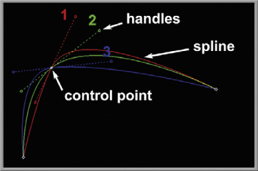
Figure 6-8 Adjusting slope
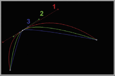
Figure 6-9 Adjusting tension
The handles can also adjust a second attribute of the spline called tension, which is shown in Figure 6-9. As the handles are shortened from position 1 to 2 to 3, the “piano wire” loses stiffness and bends more sharply around the control point. A third attribute of a spline is the angle where the two line segments meet at the control point. The angle can be an exact 180 degrees, or flat, as shown in Figure 6-8 and Figure 6-9, which makes it a continuous line. However, a “break” in the line can be introduced like Figure 6-10, putting a kink in our piano wire.
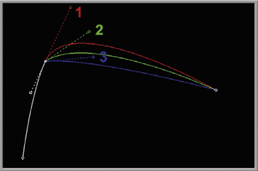
Figure 6-10 Adjusting angle
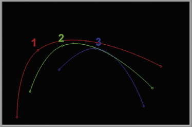
Figure 6-11 Translation
In addition to adjusting the slope, tension, and angle at each control point, the entire shape can be picked up and moved as a unit. It can be translated (moved, scaled, and rotated) taking all the control points with it as shown in Figure 6-11. This is very useful if the target has moved in the frame, such as with a camera pan, but has not actually changed shape. Of course, in the real world it will have both moved and changed shape so after the spline is translated to the new position it will also have to be adjusted to the new shape.
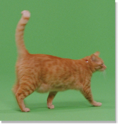
Figure 6-12 Mr. Tibbs
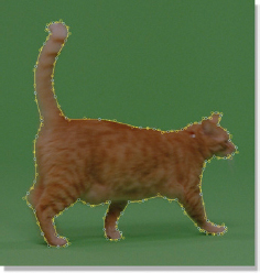
Figure 6-13 Roto spline

Figure 6-14 Finished roto
We now pull together all that we have learned about splines and how to adjust them to see how the process works over an actual picture. Our target will be the insufferable Mr. Tibbs in Figure 6-12, which provides a moving target that also changes shape frame by frame. Figure 6-13 shows the completed shape composed of splines with the many control points adjusted for slope, tension, and angle. The finished roto is shown in Figure 6-14.
(Download the folder at www.compositingVFX.com/CH06/Figure 6-12 and try your hand at rotoscoping the cat.)
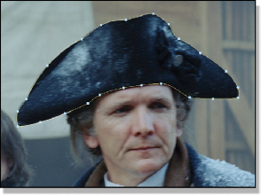
Figure 6-15 Too many control points
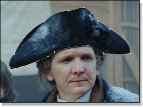
Figure 6-16 Fewest possible control points
One very important guideline when drawing a shape around a target object is to use as few control points as possible that will maintain the curvatures you need. This is illustrated by the shape used to roto the dapper hat in Figure 6-15, which uses an excessive number of control points. The additional points increase the amount of time it takes to create each keyframe because there are more points to adjust each frame. They also increase the chances of introducing chatter or wobble to the edges. Figure 6-16 shows the same shape for the hat using about half as many points. Always use the minimum number of control points possible.
6.3 ARTICULATED ROTOS
Things can get messy when rotoscoping a complex moving object such as a person walking. Trying to encompass an entire character with crossing legs and swinging arms into a single shape like the one used for the cat in Figure 6-13 quickly becomes unmanageable. A better strategy is to break the roto into several separate shapes that can be moved and reshaped independently. Many compositing programs also allow these separate shapes to be linked into hierarchical groups where one shape is the “child” of another. When the parent shape is moved the child shape moves with it. This creates a “skeleton” with moveable joints and segments rather like the target object. This is more efficient than dragging every single control point individually to redefine the outline of the target. When the roto is a collection of jointed shapes like this it is referred to as an articulated roto.
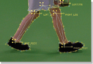
Figure 6-17 Frame 1
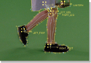
Figure 6-18 Frame 2
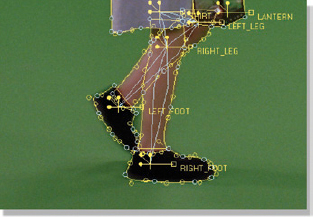
Figure 6-19 Frame 3
Figure 6-17 through Figure 6-19 illustrate a classic hierarchical setup. The shirt and lantern are separate shapes. The left and right leg shapes are “children” of the shirt, so they move when the shirt is moved. The left and right feet are children of their respective legs. The light blue lines inside the shapes show the “skeleton” of the hierarchy.
To create frame 2 (Figure 6-18) the shirt was shifted a bit, which took both of the legs and feet with it. The leg shapes were then rotated at the knee to reposition them back over the legs, and then the individual control points were touched up to complete the fit. Similarly, each foot was rotated to its new position and the control points touched up. As a result, frame 2 was made in a fraction of the time it took to create frame 1. Frame 3 was similarly created from frame 2 by shifting and rotating the parent shape, followed by repositioning the child shapes, and then touching up control points only where needed. This workflow essentially allows much of the work invested in the previous frame to be recycled into the next with just minor modifications.
There is a second, less obvious advantage to the hierarchical animation of shapes, and that is it results in a smoother and more realistic motion in the finished roto. If each and every control point is manually adjusted, small variations become unavoidable from frame to frame. After all, we are only human. When the animation is played at speed the spline edges will invariably “wobulate” (wobble and fluctuate). By translating (moving) the entire shape as a unit, the spline edges have a much smoother and more uniform motion from frame to frame.
6.4 INTERPOLATION
Time to talk temporal. Temporal, of course, refers to time. Since rotos are a frame-byframe animation, time and timing are very important. One of the breakthroughs that computers brought to rotoscoping, as we have seen, is the use of splines to define a shape. How infinitely finer to adjust a few control points to create a smooth line that contours perfectly around a curved edge rather than to draw it by hand with a pencil or ink pen. The second, even bigger breakthrough is the ability of the computer to interpolate the shapes—where the shape is only defined on selected keyframes, then the computer calculates the in-between (interpolated) shapes for you.
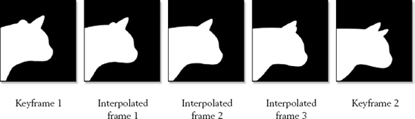
Figure 6-20 Keyframes with interpolated frames
A neat example of keyframe interpolation is illustrated in Figure 6-20. For these five frames, only the first and last are keyframes, while the three in-between frames are interpolated by the computer. The computer compares the location of each control point in the two keyframes and then calculates a new position for them at each in-between frame so they will move smoothly from keyframe 1 to keyframe 2.
There are two very big advantages to this interpolation process. First, the number of keyframes that the artist must create is often less than half the total number of frames in the shot. This dramatically cuts down on the labor that is required for what is a very labor-intensive job. Second, and perhaps even more important, is that when the computer interpolates between two shapes it does so smoothly. It has none of the jitters and wobbles that a clumsy humanoid would have introduced when repositioning control points on every frame. Bottom line—computer interpolation saves time and looks better. In fact, when rotoscoping a typical character it is normal to keyframe every other frame. The interpolated frames are then checked, and only an occasional control point touch-up applied to the in-between frames as needed.
6.5 KEYFRAMES
In the discussion above about shape interpolation the concept of the keyframe was introduced. There are many keyframing strategies one might use and choosing the right one can save time and improve the quality of the finished roto. What follows is a description of various keyframe strategies with tips on how you might choose the right one for a given shot.
6.5.1 On 2’s
A classic and often used keyframe strategy is to keyframe on 2’s, which means to make a keyframe at every other frame—frame 1, 3, 5, 7, etc. The labor is cut in half and the computer smoothes the roto animation by interpolating nicely in between each keyframe. Of course, each interpolated frame has to be inspected and any off-target control points must be nudged into position. The type of target where keyframing on 2’s works best would be something like a walking character, like the example in Figure 6-21. The action is fairly regular and there are constant shape changes, so frequent keyframes are required.
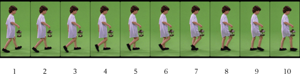
Figure 6-21 Keyframe on 2’s
On shots where the action is regular but slower it is often fruitful to try keyframing on 4’s (1, 5, 9, 13, etc.) or even 8’s (1, 9, 17, 25, etc.). The idea is to keep the keyframes on a binary number (on 2’s, on 4’s, on 8’s, etc.) for the simple reason that this ensures you will always have room for a new keyframe exactly halfway between any two existing keyframes. If you keyframe on 3’s (1, 4, 7, etc.), for example, and need to put a new keyframe between 1 and 4, the only choice is frame 2 or 3, neither of which is exactly halfway between them. If animating on 4’s (1, 5, 9, etc.) and you need to put a new keyframe between 5 and 9, frame 7 is exactly halfway between them.
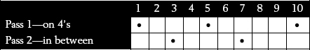
Figure 6-22 Keyframe passes on 2’s
Figure 6-22 shows the sequence of operations for keyframing a shot on 2’s in two passes by first setting keyframes on 4’s, and then in-betweening those on 2’s. Pass 1 sets a keyframe at frames 1, 5, and 9, then on a second pass the keyframes are set for frames 3 and 7. The work invested in creating keyframes 1 and 5 is partially recovered when creating the keyframe at frame 3, plus frame 3 will be smoother and more natural because the control points will be very close to where they should be and only need to be moved a small amount.
6.5.2 Bifurcation
Another keyframing strategy is bifurcation, which simply means to fork or divide into two. The idea is to create a keyframe at the first and last frames of a shot, and then go to the middle of the shot and create a keyframe halfway between them. You then go midway between the first keyframe and the middle keyframe and create a new keyframe there, then repeat that for the last frame and middle frame, and keep subdividing the shot by placing keyframes midway between the others until there are enough keyframes to keep the roto on target.
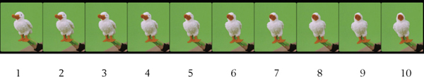
Figure 6-23 Keyframe with bifurcation
The situation where bifurcation makes sense is when the motion is regular and the object is not changing its shape very radically, like the sequence in Figure 6-23. If a keyframe were first placed at frame 1 and frame 10 then the roto checked midway at frame 5 (or frame 6, since neither one is exactly midway), the roto would not be very far off. Touch up a few control points there, and then jump midway between frame 1 and 5 and check frame 3. Touch up the control points and jump to frame 8, which is (approximately) midway between the keyframes at frame 5 and frame 10. Figure 6-24 illustrates the pattern for bifurcation keyframing.
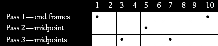
Figure 6-24 Keyframe passes with bifurcation
While you may end up with keyframes every couple of frames or so, bifurcation is more efficient than simply starting a frame 1 and keyframing on 2’s—assuming the target object is suitable for this approach. This is because the computer is interpolating the frames for you, which not only puts your shape’s control points close to the target to begin with, but it also moves and pre-positions the control points for you in a way that the resulting animation will be smoother than if you tried to keyframe it yourself on 2’s. This strategy efficiently “recycles” the work invested in each keyframe into the new in-between keyframe.
6.5.3 Extremes
Very often the motion is smooth but not regular, such as the gyrating airplane in Figure 6-28 which is bobbing up and down as well as banking. In this situation a good strategy is to keyframe on the extremes of the motion. To see why, consider the airplane path plotted in Figure 6-25. The large dots on the path represent the airplane’s location at each frame of the shot. The change in spacing between the dots reflects the change in the speed of the airplane as it maneuvers. In Figure 6-26 keyframes were thoughtlessly placed at the first, middle, and last frames, represented by the large red dots. The small dots on the thin red line represent where the computer would have interpolated the rotos using those keyframes. As you can see, the interpolated frames are way off the true path of the airplane.
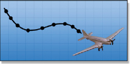
Figure 6-25 Airplane path
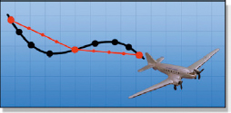
Figure 6-26 Wrong keyframes
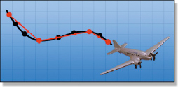
Figure 6-27 Extreme keyframes
However, in Figure 6-27 keyframes were placed on the frames where the motion extremes occurred. Now the interpolated frames (small red dots) are much closer to the true path of the airplane. The closer the interpolation is to the target, the less work you have to do and the better the results. To find the extremes of a shot, play it in a viewer so you can scrub back and forth to make a list of the frames that contain the extremes. Those frames are then used as the keyframes on the first roto pass. The remainder of the shot is keyframed using bifurcation.
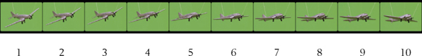
Figure 6-28 Keyframe on extremes
Referring to a real motion sequence in Figure 6-28, the first and last frames are obviously going to be extremes so they go on our list of keyframes. Looking at the airplane’s vertical motion it appears to reach its vertical extreme on frame 3. By placing keyframes on frame 1, 3, and 10 we stand a good chance of getting a pretty close fit when we check the interpolation at frame 7 (see Figure 6-29). If the keyframe were placed at the midpoint on frame 5 or 6, instead of the motion extreme at frame 3, the roto would be way off when the computer interpolates it at frame 3.
(Download the folder at www.compositingVFX.com/CH06/Figure 6-28 and try your hand at rotoscoping the airplane.)
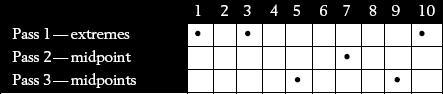
Figure 6-29 Keyframe passes using extremes
Regardless of the keyframe strategy chosen, when the roto is completed it is time for inspection and touch-up. The basic approach is to use the matte created by the roto to set up an “inspection” version of the shot that highlights any discrepancies in the roto, and then go back in and touch up those frames. After the touch up pass, one final inspection pass is made to confirm all is well.
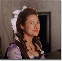
Figure 6-30 Film frame
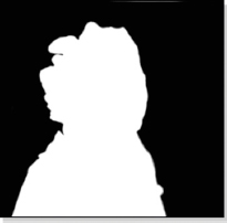
Figure 6-31 Roto
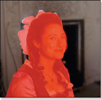
Figure 6-32 Inspection
Figure 6-30 through Figure 6-32 illustrate a typical inspection method. The roto in Figure 6-31 was used as a mask to composite a semi-transparent red layer over the film frame in Figure 6-32 to highlight any discrepancies in the roto. It shows the roto falls short on the white bonnet at the top of the head and overshoots on the side of the face. The roto for this frame is then touched up and the inspection version made again for one last inspection to confirm all fixes and no new problems. Using this red composite for inspection will probably not work well when rotoscoping a red fire engine in front of a brick building. Feel free to modify the process and invent other inspection setups based on the color content of your personal shots.
6.6 MOTION BLUR
One of the historical shortcomings of the roto process has been the lack of motion blur. A roto naturally produces clean sharp edges like all the examples we have seen so far, but in the real world moving objects have some degree of motion blur where their movement has smeared their image on the film or in the video. Figure 6-33 shows a rolling ball of yarn with heavy motion blur. The solution is an inner and outer spline that defines an inside edge that is 100% solid and an outside edge that is 100% transparent, like the example in Figure 6-34. The roto program then renders the matte as 100% white from the inner spline graduating off to black at the outer spline. This produces a motion-blurred roto like the one shown in Figure 6-35. Even if there is no apparent motion blur in the image it is often beneficial to gently blur the rotos before using them in a composite to soften their edges a bit, especially in film work.
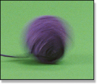
Figure 6-33 Motion blurred target
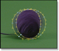
Figure 6-34 Shape with inner and outer splines

Figure 6-35 Resulting motion blurred roto
One problem that these inner and outer splines introduce, of course, is that they add a whole second set of spline control points to animate, which increases the labor of an already labor-intensive process. However, when the target object is motion blurred there is no choice but to introduce motion blur in the roto as well.
A related issue is depth of field, where all or part of the target might be out of focus. The bonny lass in Figure 6-4, for example, actually has a shallow depth of field so her head and near shoulder are in focus but her far shoulder is noticeably out of focus. One virtue of the inner and outer spline technique is that edge softness can be introduced only and exactly where it is needed so the entire roto does not need to be blurred. This was done for her roto in Figure 6-5.
6.7 SEMI-TRANSPARENCY
Another difficult area for rotoscoping is a semi-transparent object. The main difficulty with semi-transparent objects is that their transparency is not uniform—some areas are denser than others. The different levels of transparency in the target mean that a separate roto is required for each level. This creates two problems. The first is that some method must be devised for reliably identifying each level of transparency in the target so it may be rotoscoped individually, without omission or overlap with the other regions. Second, the roto for each level of transparency must be made unique from the others in order to be useful to the compositor.
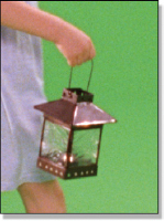
Figure 6-36 Semi-transparent lantern
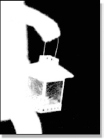
Figure 6-37 Semi-transparent matte
A good example of these issues is the lantern being carried by our greenscreen boy. A close up is shown in Figure 6-36. When a matte is created using a high-quality digital keyer (Figure 6-37), the variable transparency of the frosted glass becomes apparent. If this object needed to be rotoscoped to preserve its transparency we would need to create many separate roto layers, each representing a different degree of transparency. This is usually done by making each roto a different brightness—a dark gray roto for the very transparent regions, medium brightness for the medium transparency, and a bright roto for the nearly solid transparency. While it is a hideous task, I have seen it done successfully.