The focus of Chapter 3 was on the analysis of kinematically driven systems in which all the degrees of freedom are specified. Since the system configuration can be completely determined when the degrees of freedom are known, the analysis of kinematically driven systems leads to a system of algebraic equations that can be solved for the coordinates, velocities, and accelerations without the need for a force analysis. However, if one or more of the system degrees of freedom are not known a priori, the force analysis becomes necessary and the system equations of motion must be formulated to obtain a number of equations equal to the number of the unknown variables. In the case of unconstrained motion, the equations of motion of the system take a simple known form defined by Newton-Euler equations, and therefore, the selection of the system coordinates is not the subject of much argument. In the case of constrained multibody dynamics, on the other hand, different numbers of coordinates can be selected, leading to different forms of the dynamic equations. Some formulations that employ redundant coordinates lead to a relatively large system of equations expressed in terms of the constraint forces, while some other formulations lead to a minimum set of differential equations of motion expressed in terms of the degrees of freedom. Since the degrees of freedom, by definition, are independent and are not related by kinematic relationships, it is expected that the constraint forces are automatically eliminated when the equations of motion are formulated in terms of the degrees of freedom.
Much of the research on computational dynamics has been focused on the selection of the coordinates and on studying the advantages and drawbacks of different formulations. Despite the drawback of increasing the number of equations and the dimensionality of the problem, the use of redundant coordinates instead of using the degrees of freedom has the advantage of increasing the generality of the formulation and achieving a sparse matrix structure. On the other hand, the formulations in terms of the degrees of freedom have the advantage of reducing the number of equations at the expense of increasing the complexity of the inertia and force coefficients that appear in these equations. In this chapter, a brief introduction to some forms of the dynamic equations of motion is presented. D'Alembert's principle is introduced and its use in formulating the equations of motion of mechanical systems is demonstrated using simple examples. Different matrix formulations for the equations of motion are then obtained using D'Alembert's principle. Some of these formulations lead to a large number of equations which include the constraint forces, while others lead to a smaller set of equations which do not include any constraint forces. Among the matrix formulations presented in this chapter are the augmented formulation, the embedding technique, and the amalgamated formulation. This chapter also includes a brief discussion on the analysis of open- and closed-chain systems. The material presented in this chapter can be considered as an introduction to some of the concepts and computational methods which are discussed in more detail in the remainder of the book. Simple procedures are used in this chapter to introduce different formulations; a more systematic and rigorous development of some of these formulations is presented in the following chapters.
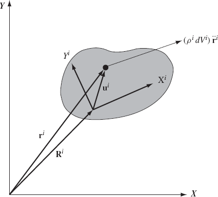
As demonstrated in Chapter 3, the unconstrained planar motion of a rigid body can be described using three independent coordinates. As shown in Fig. 1, two coordinates Rix and Riy can be used to define the translation of the reference point and one coordinate θi defines the orientation of the rigid body coordinate system XiYi with respect to the global coordinate system XY. Associated with these three coordinates, there are three independent differential equations that govern the unconstrained planar motion of a rigid body. If the reference point is selected to be the center of mass of the body, these equations can be written as
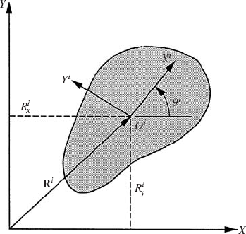
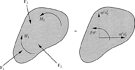
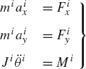
where mi is the total mass of the rigid body, Ji is the mass moment of inertia defined with respect to the center of mass, aix and aiy are the components of the absolute acceleration of the center of mass of the body,
Example 4.1
Figure 3 shows a simple system that consists of two moving bodies. Body 1 is a slider block that has a specified motion defined by the function z(t). Body 2 is a uniform slender rod that has mass m2, mass moment of inertia about its center of mass J2, and length l. The rod that is subjected to the external moment M2 is connected to the sliding block by a pin joint at O.
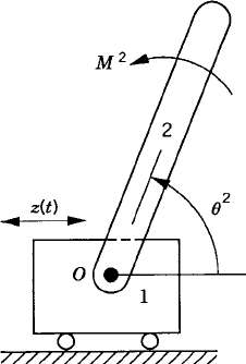
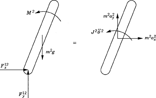
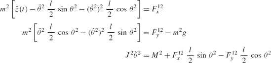
Figure 4 shows a free-body diagram for the rod. By applying Eq. 1, one obtains
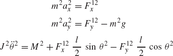
where F12x and F12y are the joint reaction forces at the pin joint. Since the motion of the sliding block is specified, the system has only one degree of freedom, which can be considered as the angular orientation of the rod θ2.
If the applied forces and moments are given, as in the case of the forward dynamic analysis, the direct application of the Newton-Euler equations, in this example, leads to three differential equations of motion which are expressed in terms of five unknown acceleration components and reaction forces. These unknowns are a2x, a2y,
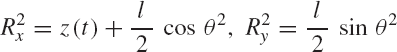
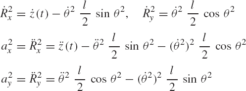
which upon differentiation once and twice lead to
Using the expressions for a2x and a2y in these equations, a forward elimination process can be applied to reduce the number of unknowns in the equations of motion. To this end, the expressions for a2x and a2y in the preceding equations are substituted into the differential equations of motion. This leads to
These are three equations that can be solved for the three unknowns
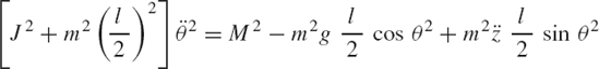
This equation does not contain the joint reaction forces and can be solved for the angular acceleration
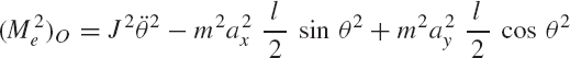
Another alternative for obtaining the preceding equation is to apply D'Alembert's principle. According to this principle, the moment of the inertia forces about O is equal to the moment of the externally applied forces about the same point. This leads to one differential equation that does not include the joint reaction forces. The moment of the inertia (effective) forces about point O is
The moment of the externally applied forces about O is
D'Alembert's principle implies that
or
Substituting for the accelerations of the center of mass of the rod using the previously obtained kinematic relationships, one obtains
which is the same equation obtained previously by eliminating the joint reaction forces.
It is clear from the analysis presented in Example 1 that the direct application of Newton's second law or D'Alembert's principle to derive the dynamic conditions for a body in a mechanical system leads to a set of equations expressed in terms of the accelerations, the applied forces and moments, and the joint reaction forces. If the applied forces and moments are known, the resulting dynamic equations can be considered as a linear system of algebraic equations that can be solved for the accelerations and the joint reaction forces. The accelerations can be integrated forward in time in order to determine the coordinates and velocities. There are, however, several methods for formulating the acceleration equations. These methods are discussed briefly in this chapter to provide a motivation for the study of the materials covered in the following chapters. Before these different methods are presented, we first show in the following section how to use D'Alembert's principle to derive the Newton-Euler equations in the case of rigid bodies.
The Newton-Euler equations defined in Eq. 1 can be derived in a straightforward manner by applying D'Alembert's principle. In fact, D'Alembert's principle can be used to develop a set of equations, which do not restrict the choice of the reference point to be the center of mass of the body. In this section, the derivations of both Newton and Euler equations for rigid bodies are presented.
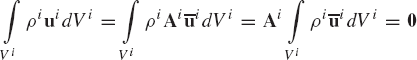
As shown in Fig. 5, a rigid body i can be considered to consist of a large number of particles, each of which has mass ρidVi where ρi is the mass density, and dVi is the infinitesimal volume. The inertia force of a particle whose position vector ri is then equal to
In this equation, Fi is the vector of resultant forces acting on the body. The preceding equation is general and allows using any point as the reference point. In the planar analysis, Eq. 2 has two scalar equations. Recall that the absolute acceleration of an arbitrary point on the rigid body i can be written as
where Ri is the global position vector of the reference point on the body, ωi and αi are, respectively, the angular velocity and angular acceleration vectors of the body,
Substituting Eq. 3 into Eq. 2 and using the identity of Eq. 4 and the fact that ωi and αi do not depend on the location of the arbitrary point, one obtains
The vector of the center of mass acceleration
Eq. 5 yields
This is the Newton equation of motion for the rigid body i, it is the same as the first two scalar equations given by Eq. 1. It is worth mentioning that Eq. 7 is a special case of Eq. 2. In Eq. 2, the reference point can be an arbitrary point; while in Eq. 7, the reference point must be the center of mass of the body.
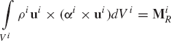
The third equation in Eq. 1 is Euler equation. This equation can be obtained from D'Alembert's principle by treating the inertia forces as the applied forces. To this end, it is assumed again that the rigid body i consists of a large number of particles. The moment of the inertia force of a particle about the reference point is defined as
In this equation, MiR=[0 0 Mi]T is the vector of the resultant moment about the reference point. This vector has one nonzero component only because the case of planar analysis is considered. Three-dimensional vectors are used in this section because of the convenience of using the cross product, which is defined for three-dimensional vectors only.
It is important to mention that Eq. 8 does not restrict the choice of the reference point to the center of mass. In this equation, any point on the body can be used as the reference point. The choice of the reference point as the center of mass, however, leads to significant simplifications in the resulting dynamic equation. Note also that in the case of planar motion, Eq. 8 reduces to only one nontrivial scalar equation that represents the moment about the Zi axis since ui and
In order to obtain Euler equation, the reference point is chosen to be the body center of mass. Substituting Eq. 3 into Eq. 8, and using the identity of Eq. 4, and the fact that ui and ωi × (ωi × ui) are two parallel vectors, one obtains
Note that in the case of planar motion,
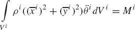
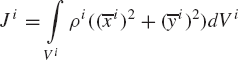
Note that the mass moment of inertia of the body Ji is defined as
It follows from the preceding two equations that
This is Euler equation, the third equation of Eq. 1.
In deriving the Newton-Euler equations using D'Alembert's principle, it is assumed that the reference point is the body center of mass. This assumption leads to significant simplifications of the resulting equations of motion. It also leads to a formulation that does not include inertia coupling between the translation of the center of mass and the rotation of the body. If the center of mass is not considered as the reference point, Eqs. 2 and 8 represent the equations of motion of the body. One can show in this more general case that the resulting equations include inertia coupling between the translation of the reference point and the rotation of the body. In the case of rigid body dynamics, there is no clear advantage of using a reference point different from the body center of mass since the resulting equations become more complex. Similar comment applies to the case of spatial analysis, where a procedure similar to the one described in this section can be used to develop the three-dimensional Newton-Euler equations that govern the spatial motion of rigid bodies. This subject will be discussed in detail in a latter chapter of this book.
Mechanical joints and specified motion trajectories in multibody systems impose restrictions on the motion of the system components. Because of the kinematic constraints of the joints and specified motion trajectories, the selection of coordinates and the form of the equations of motion is not a trivial task and has been the subject of extensive research in the area of computational multibody system dynamics. The efficiency, generality, and numerical algorithm of a solution procedure strongly depend on the choice of the coordinates and the resulting form of the equations of motion. Joints and specified motion trajectories introduce constraint forces that may explicitly appear in the formulation or can be systematically eliminated by expressing the dynamic equations in terms of a chosen set of independent coordinates or degrees of freedom. As will be demonstrated in this section using a simple example, the number of independent constraint forces is always equal to the number of independent constraint equations, which is equal to the number of dependent coordinates. Obviously, if there are no constraints between the coordinates, there are no constraint forces and there are no dependent coordinates. This simple fact is crucial in understanding the basis of different forms of the dynamic equations of motion.
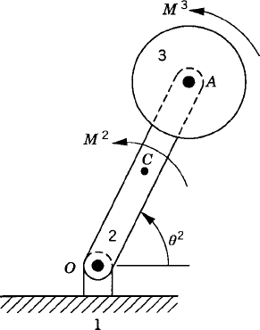
Consider the simple system shown in Fig. 6. This system consists of the ground denoted as body 1, a rod OA denoted as body 2, and a disk denoted as body 3. The rod is connected to the ground by a pin joint at O, while the disk is connected to the rod by a pin joint at A. The rod is assumed to be uniform and its length is l. Figures 7a and b show the free-body diagrams of the rod and the disk. It is clear from these diagrams that
These are six dynamic equations in 10 unknowns; six acceleration components and four components of the reaction forces. Since the system has two degrees of freedom, the six acceleration components can be expressed in terms of two independent accelerations using the kinematic constraint equations at the acceleration level. In this example, the accelerations of the centers of mass of bodies 2 and 3 can be written in terms of the angular acceleration of body 2. Since point O is a fixed point, the absolute accelerations of the centers of mass of bodies 2 and 3 can be written as
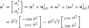
where u2CO and u2AO are the vectors that define the locations of the centers of the rod and the disk with respect to point O. Note that the number of constraints of Eqs. 14 and 15 is equal to the number of the four independent reaction forces of the two pin joints. This number is also equal to the number of dependent coordinates used to formulate the equations of motion of the system.
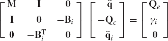
In general, one can show that for any given constrained multibody system, the direct application of Newton-Euler equations leads to a system of differential equations that can be written in the following general matrix form:
In this equation, M is the mass matrix of the system, q is the vector of the system coordinates, Qe is the vector of applied forces, and Qc is the vector of constraint forces. The number of scalar equations in the matrix equation of Eq. 16 is equal to the number of accelerations. In the case of forward dynamics, the applied forces defined by the vector Qe are given. The unknowns in this case of forward dynamics are the accelerations and the constraint forces that enter into the formulation of the vector Qc. The number of independent constraint forces is equal to the number of the algebraic equations that represent the constraints imposed on the motion of the system. These algebraic constraint equations, as demonstrated in the preceding chapter, can be written in the following vector form:
The second derivatives of these constraint functions with respect to time define the constraint equations at the acceleration level, which in the example discussed in this section are equivalent to Eqs. 14 and 15.
In the special case of the example discussed in this section, one can recognize the vector of coordinates q as
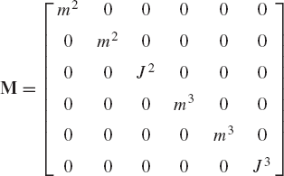
The mass matrix M can be defined using the coefficients of the accelerations in Eq. 13 as
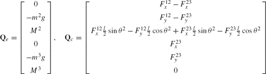
The vector of applied forces Qe and the vector of constraint forces Qc can also be defined using Eq. 13 as
For this example, the constraints of Eq. 17 are defined as
In these constraint equations, Ri = [Rix Riy]T, i = 2, 3; and
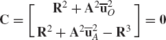
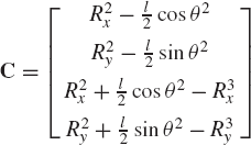
Using these definitions (Eq. 22), the system constraint equations at the position level, as defined by Eq. 21, can be written more explicitly as
There are several matrix methods for solving Eqs. 16 and 17 for the accelerations and the joint reaction forces. In this chapter we discuss briefly some of the matrix methods that are used to formulate the acceleration equations. Among these methods are the augmented formulation, the embedding technique, and the amalgamated formulation. Equations 13-15, which describe the dynamics of the system shown in Fig. 6, are used as an example to illustrate the concepts underlying these methods.
In the augmented formulation, the constraint forces explicitly appear in the dynamic equations, which are expressed in this case, in terms of redundant coordinates. The constraint relationships are used with the differential equations of motion to solve for the unknown accelerations and constraint forces. This approach leads to a sparse matrix structure and can be used as the basis for developing more general multibody system codes. Nonetheless, the augmented formulation has the drawback of increasing the problem dimensionality and it requires more sophisticated numerical algorithms to solve the resulting system of differential and algebraic equations, as discussed in the following chapters. In this section, the simple example discussed in the preceding section is used to introduce the augmented formulation.
In the augmented formulation, Eqs. 13-15 are combined in order to form a system of 10 scalar equations that can be solved for the 10 unknown accelerations and joint reaction forces. This leads to the following system:
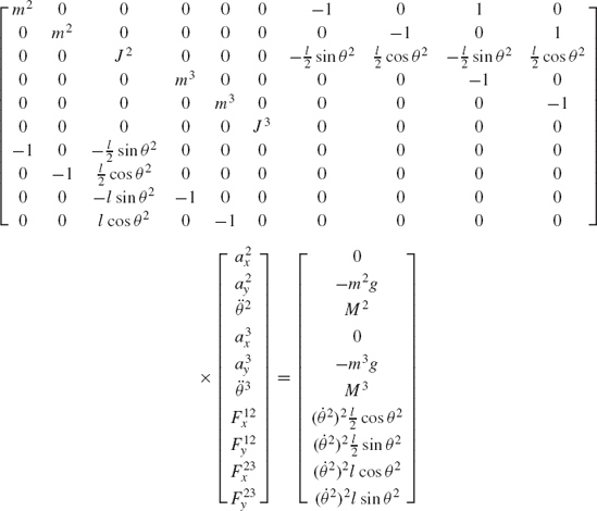
Note that in this form of the equations of motion, the constraint equations are not used to eliminate the dependent accelerations. As a result, a relatively large system of equations is obtained. It is also clear that the coefficient matrix in this equation is a sparse matrix since it has many zero elements. Sparse matrix techniques can then be used to solve the preceding form of the dynamic equations efficiently in order to determine the accelerations and the constraint forces.
A more systematic and general procedure for developing the augmented equations of motion is based on the Lagrangian dynamics. In the Lagrangian approach, the technique of Lagrange multipliers is used to define generalized constraint forces and to obtain an augmented formulation in which the coefficient matrix is symmetric.
Equation 24 can be used to introduce the powerful technique of Lagrange multipliers and to demonstrate the basic differences between the Lagrangian mechanics and the Newtonian mechanics. In the Lagrangian mechanics, one does not need to make cuts at the joints and be concerned from the outset with the actual reaction forces. Instead, the equations of motion can be developed using the assembled system and the connectivity conditions (constraint equations). In order to demonstrate this approach, the example shown in Fig. 6 is used again. To this end, the Jacobian matrix of the constraints of Eq. 23 is written as
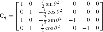
The columns of this constraint Jacobian matrix correspond to the vector of the system coordinates defined in Eq. 18. Differentiating the constraint functions of Eq. 17 twice with respect to time, one obtains
Using the constraints of Eq. 23, one can show that
After developing the expressions for the constraint equations and their second derivatives with respect to time, we return again to Eq. 24. We note that this equation can be, after multiplying some equations by a negative sign, rewritten as
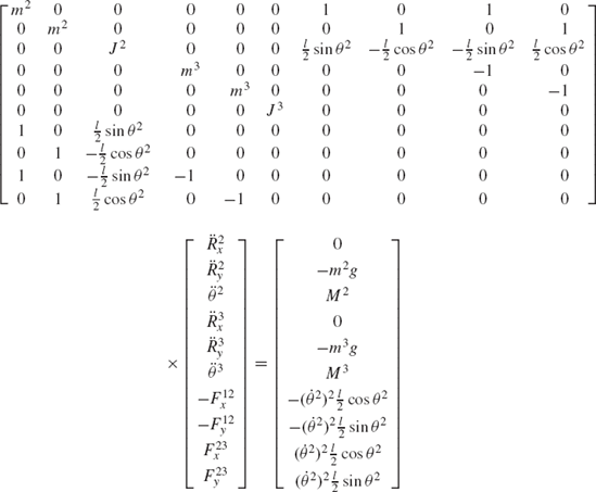
By using the expressions given in Eqs. 19, 20, 25 and 27, it is clear that Eq. 28 can be written in the following form:
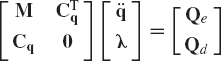
In this equation
While in this section, the simple example of Fig. 6 is used to derive Eq. 29; this equation is general and can be applied to any system subject to constraints. The coefficient matrix in this equation is always symmetric and positive definite for a well-posed problem. The vector λ is called the vector of Lagrange multipliers. In this simple example, Lagrange multipliers take a simple form expressed in terms of the actual reaction forces at the joints. While this is not always the case, the constraint forces associated with the system coordinates can always be written as
The number of Lagrange multipliers is always equal to the number of constraint equations, which is equal to the number of dependent variables. Lagrange multipliers, which replace the independent reaction forces, are treated as unknowns, and therefore, one does not need to be concerned with the reaction forces from the outset. Instead, in the Lagrangian formulation, one needs to write the constraint equations (connectivity conditions) and use them to determine the constraint Jacobian matrix and the vector Qd as was described in Chapter 3 of this book. The use of the constraint equations instead of the reaction forces, in addition to being one of the fundamental differences between the Lagrangian and Newtonian mechanics, allows for the systematic development of general computer algorithms that can be used in the analysis of complex and large-scale multibody systems. More detailed discussion on the augmented form of the equations of motion as given in Eq. 29 will be presented in later chapters of this book.
The approach discussed in this section is not one of the basic methods used in computational dynamics and is not widely used for solving multibody system applications. It is discussed here to serve as an intermediate step and as a brief introduction to the more widely used technique, the embedding technique, introduced in the following section. In this section, the constraint equations are used to eliminate the dependent accelerations leading to a system of equations that can be solved for the independent accelerations and the constraint forces. To demonstrate the use of this procedure, we consider the same example that was discussed in the preceding sections.
To solve Eqs. 13-15, the kinematic relationships of Eqs. 14 and 15 are used to eliminate the dependent components of the accelerations. To this end, we substitute Eqs. 14 and 15 into Eq. 13, and arrange the terms to obtain
These six equations, which have two unknown angular accelerations and four unknown reaction forces, can be written in the following matrix form:
where
and

The system of matrix equations defined by Eq. 33 can be solved for the unknown independent angular accelerations and the joint reaction forces. The dependent accelerations can be determined using the constraint equations at the acceleration level (Eqs. 14 and 15).
As previously mentioned in this chapter, the vector of constraint forces associated with the system coordinates can be expressed in terms of multipliers, called Lagrange multipliers λ (see Eq. 31). The number of these multipliers is equal to the number of constraint equations and is also equal to the number of independent constraint forces. In order to develop a general procedure for the elimination of the dependent accelerations, Eq. 31 is substituted into Eq. 16. This leads to
Note that this equation is the same as the equation defined in the first row in Eq. 29. In the case of forward dynamics, the unknowns in Eq. 36 are the vector of accelerations
In this equation, the matrix Bi is called the velocity transformation matrix. This matrix plays a central role in the embedding technique discussed in the following section. The vector γi is always quadratic in the velocities. Substituting Eq. 37 into Eq. 36 and arranging the terms, one obtains
This system of equations, which has a square coefficient matrix, can be solved for the independent accelerations
In order to demonstrate the formulation of the velocity transformation matrix Bi and the vector γi used in Eq. 37, we select the vector of independent coordinates as qi = [θ2 θ3]T and use the results of Eqs. 14 and 15 to write
Using this equation, the velocity transformation matrix Bi and the quadratic velocity vector γi are recognized as
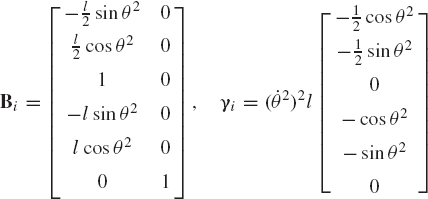
Note that the product MBi, which appears in Eq. 38, is a 6 × 2 matrix and it is left to the reader to verify that this product is the same as the first two columns of the coefficient matrix that appears in Eq. 33. The matrix CTq, on the other hand, is a 6 × 4 matrix since the number of constraint equations is 4 and the number of coordinates is 6. One can show by substituting the results of Eq. 40 into Eq. 38 and using the definition of Lagrange multipliers given for this example by Eq. 30 that the use of Eq. 38 will lead to the same equations as presented in Eq. 33.
In the formulations discussed in the preceding sections, the equations of motion are expressed in terms of the constraint forces. By using the embedding technique, the constraint forces can be eliminated systematically and a number of equations of motion equal to the number of the system degrees of freedom can be obtained. To obtain this minimum set of differential equations, it is necessary to use the velocity transformation matrix defined in the preceding section. This matrix can be defined systematically when the total vector of the system accelerations is expressed in terms of the independent accelerations. In the embedding technique, Eq. 38 is premultiplied by the transpose of the velocity transformation matrix Bi. This leads to
The following important identity holds
This is an expected result that will be demonstrated using the two-body example discussed in this chapter. Substituting Eq. 42 into Eq. 41, one obtains
This equation can be written as
where
Note that Eq. 44 does not include any constraint forces, and the number of the scalar equations in this matrix equation is equal to the number of the system degrees of freedom. Using the procedure described in this section, one can always obtain a number of equations equal to the number of degrees of freedom, and these equations do not include any constraint forces. The matrix Mi is the generalized inertia matrix associated with the system degrees of freedom, and the vector Qi is the vector of generalized forces associated with these degrees of freedom.
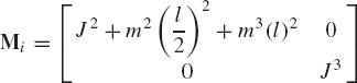
In order to demonstrate the use of the embedding technique described in this section, we return to the two-body example shown in Fig. 6. The constraint Jacobian matrix and the velocity transformation matrix of this system are given, respectively, by Eqs. 25 and 40. Using these two equations, one can show that BTiCTq=0. Using the definition of the mass matrix of Eq. 19 and the velocity transformation matrix of Eq. 40, one can show that the generalized mass matrix Mi defined in Eq. 45 is given as
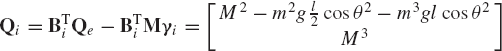
Using the definitions of Eqs. 20 and 40, Eq. 45 can be used to define the vector Qi as
The equations of motion of the two-body system can then be obtained using Eq. 44 as
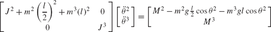
These equations, which do not include constraint forces, can be solved for the independent angular accelerations. The total vector of the system accelerations can be determined using Eq. 37. Knowing all the accelerations, one can substitute into the equations of motion before eliminating the dependent accelerations in order to determine the constraint forces.
As previously mentioned, the velocity transformation matrix Bi plays a fundamental role in the embedding formulation. This matrix allows for the systematic elimination of the constraint forces as demonstrated in this section. By so doing, a minimum set of dynamic differential equations of motion can be defined and expressed solely in terms of the system degrees of freedom. In Chapter 5, a systematic procedure based on the concept of the virtual displacement is used to define the velocity transformation matrix. The principle of virtual work is also used in Chapter 5 to systematically develop the embedding technique, which is introduced in this section using the familiar Newtonian mechanics approach.
Another method for solving for the accelerations and the joint reaction forces is to obtain a very large system of loosely coupled algebraic equations. To this end, Eq. 16 is reproduced here for convenience
It was previously shown that the vector of accelerations can be expressed in terms of the independent accelerations using Eq. 37, which is repeated here
One can verify by using Eq. 42 that
where Bi is the velocity transformation matrix.
Equations 49-51 can be combined in one matrix equation to yield
This large system, which has a sparse symmetric coefficient matrix, can be solved for the accelerations and the joint forces as well as the independent accelerations.
As will be demonstrated in Chapter 6, one of the advantages of using the augmented formulation is that open and closed kinematic chains can be treated alike. When other methods are used, special attention must be given to closed kinematic chains, which can have singular configurations, as also discussed in Chapter 6. In this section and the following section, we discuss some of the basic differences between open and closed chains to demonstrate the difficulties encountered in the analysis of closed chains and to have an appreciation of some of the advantages of the technique of Lagrange multipliers, which is discussed in more detail in Chapter 6.
Two methods are used in this section to develop the dynamic equations of open-chain systems. In the first method, the dynamic conditions are developed for each body in the system, leading to a set of equations expressed explicitly in terms of the joint reaction forces. The resulting number of equations is equal to the number of the system degrees of freedom plus the number of the joint reaction forces. These equations can be solved for the reaction forces in addition to a number of unknowns equal to the number of degrees of freedom of the system as previously demonstrated in Section 6 of this chapter. For example, if all the external forces are specified, the resulting dynamic equations can be solved for the reaction forces and a number of unknown accelerations equal to the number of degrees of freedom of the system. In the second method discussed in this section, cuts are made at selected joints and the dynamic conditions are formulated for selected subsystems leading to minimum number of differential equations. The number of these equations, which do not contain the joint reaction forces, is equal to the number of degrees of freedom of the system. Clearly, this minimum number of equations can be obtained using the first approach by eliminating the joint reaction forces, as demonstrated in Section 7.
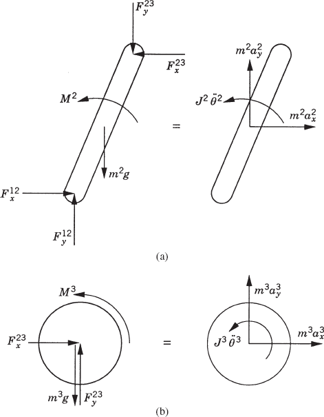
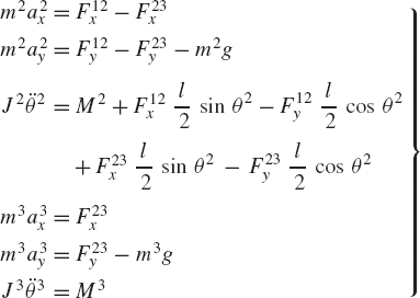
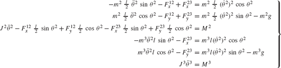
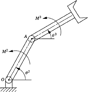
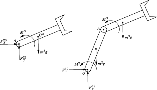
First, we consider the formal application of the dynamic conditions to each body in the system. The two-degree-of-freedom two-arm manipulator system shown in Fig. 8 is used. Body 1 represents the ground or the fixed link. Body 2 represents the first movable link in the manipulator, and its orientation is defined by the angle θ2. Body 3 represents the second movable link in the manipulator, and the orientation of this body is defined by the angle θ3. Let M2 and M3 be the joint torques that act on body 2 and body 3, respectively. Figure 9 shows the free-body diagrams of the two bodies. From this figure the dynamic conditions of body 2 are
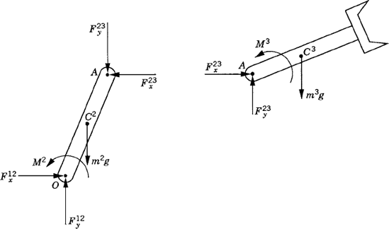
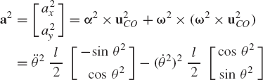
where m2 and J2 are, respectively, the mass and mass moment of inertia of body 2; a2x and a2y are the components of the acceleration of the center of mass of this body, g is the gravity constant; and Fijx and Fijy are the components of the reaction force acting on body i as the result of its connection with body j. In a similar manner, one may write the dynamic equations for body 3 as
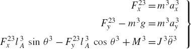
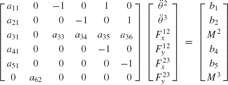
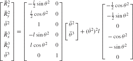
In this section, the case of the inverse dynamics (kinematically driven system) is considered to focus the attention on the basic differences between the open and closed kinematic chains. In this case, the motion of the system is assumed to be known and the goal is to solve for the external and joint forces. Assuming that the accelerations are known, Eqs. 53 and 54 can be arranged and combined in one matrix equation as
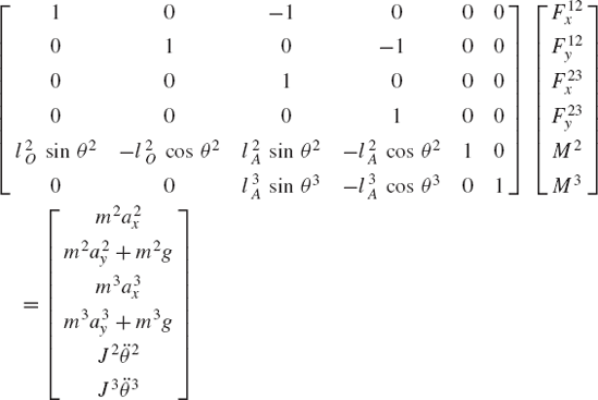
which can be written as
where the coefficient matrix A is defined as
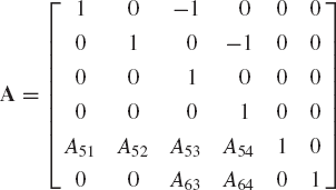
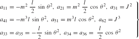
and the vectors x and b are
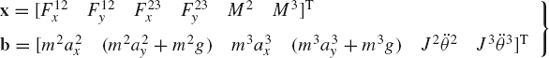
In these equations
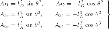
and liO and liA are the distances of points O and A from the center of mass of link i.
The solution of Eq. 56 is given by x = A−1b, where the matrix A−1 is the inverse of the matrix A given by
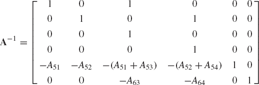
It follows that the solution x is given as
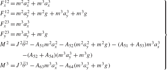
The last two equations in Eq. 61 do not include the reaction forces which are given by the first four equations.
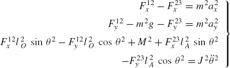
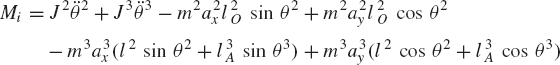
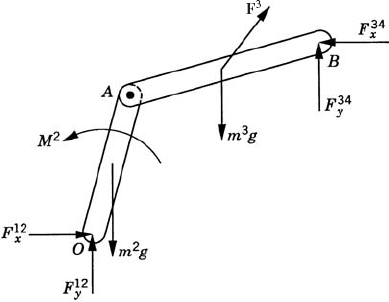
In the analysis of open-chain systems, the last two equations in Eq. 61 can be obtained directly, without considering the internal reaction forces by studying the equilibrium of selected subsystems, as shown in Fig. 10. For example, we may consider the dynamic equilibrium of link 3 in our example and take the moment about point A for both the systems of external and effective forces. The moments of the external forces and moments are
The moments of the inertia forces about A are
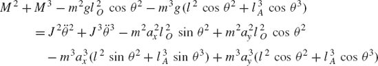
Applying D'Alembert's principle, which implies that the inertia or effective moment is equal to the moment of the applied forces, one obtains
which can be rearranged as
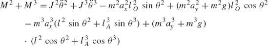
This equation is the same as the last equation in Eq. 61. A second equation can be obtained by studying the equilibrium of bodies 2 and 3 together, as shown in Fig. 10. By taking the moments about point O, we can eliminate the internal reactions. For the external forces and moments, we have
The moments of the inertia forces and moments about O yield
Thus, the dynamic equilibrium condition for this subsystem is
which can be rearranged and written as
Equations 65 and 69 represent the dynamic conditions for the two-degree-of-freedom system. They are two independent equations that can be solved for two unknowns. It is clear that upon subtracting Eq. 65 from Eq. 69, one obtains
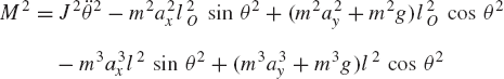
This is the same equation as the fifth equation in Eq. 61 obtained here from the application of the dynamic conditions to each body in the system separately. Therefore, the two methods discussed in this section lead to the same results. The second method, however, represents the foundation for some of the recursive methods, which allow elimination of the joint reaction forces in the analysis of open kinematic chains. Another systematic and straightforward approach to obtain Eqs. 65 and 70, which are the same as the last two equations of Eq. 61, is to use the principle of virtual work in dynamics, which will be discussed in the following chapter.
It was demonstrated by the analysis presented in the preceding section that the joint reaction forces can be eliminated from the dynamic equations of open-chain systems by considering the equilibrium of selected subsystems. The analysis that follows will demonstrate the differences between open- and closed-chain systems, and as in the case of open-chain systems, two methods will be considered. In the first method, the dynamic equations are developed for each body in the system leading to a set of equations which are explicit functions of the joint reaction forces. In the second approach, cuts are made at selected secondary joints and the dynamics of the resulting subsystems is examined.
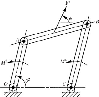
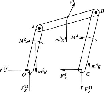
As in the case of open-chain systems, the dynamic equations of a closed-chain system are first obtained by developing the dynamic equations of each body in the system separately. This leads to a number of equations equal to the number of reaction forces plus the number of degrees of freedom of the system. To demonstrate the use of this approach, we consider the closed-chain four-bar linkage shown in Fig. 11. The fixed link is denoted as body 1, the crankshaft is denoted as body 2, the coupler is denoted as body 3, and the rocker is denoted as body 4. The dynamic equations of the crankshaft, which is subjected to an external moment M2 as shown in Fig. 12, are given by the following three equations:

where the moment equation is defined with respect to the center of mass of the crankshaft.
The coupler, as shown in Fig. 12, is subjected to an external force F3 that acts at its center of mass. The dynamic equations for the coupler can be written as
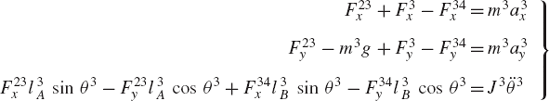
where F3x and F3y are the components of the external force vector F3.
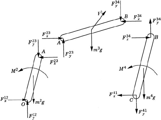
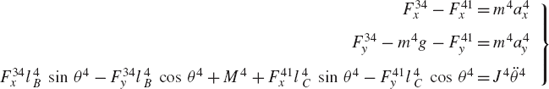
As shown in Fig. 11, the rocker is subjected to the external moment M4. The dynamic equations of the rocker are
The dynamic conditions of the four-bar mechanism lead to nine equations that can be solved for nine unknowns; eight of them are the reaction forces at the joints. We arrange these nine equations presented in the preceding three equations and write them in the following matrix form:
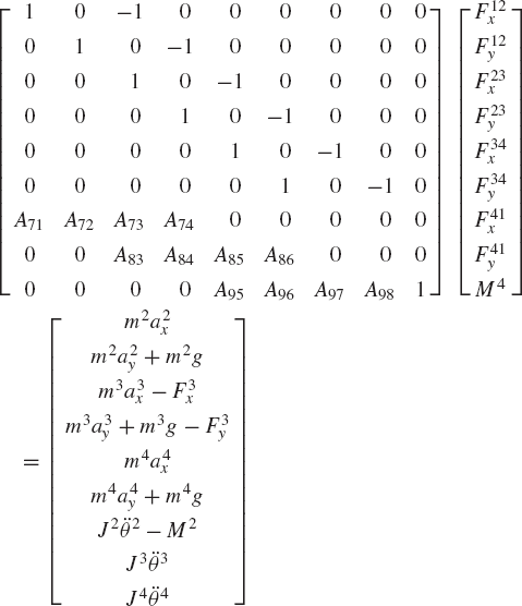
where
Equation 74 can be written as
where A is the coefficient matrix
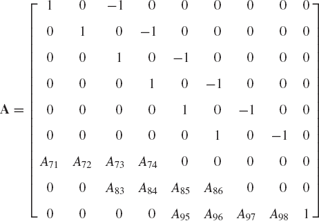
and the vectors x and b are
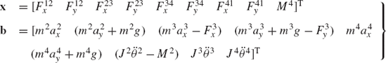
The solution of Eq. 76 can be defined as in the case of the open chain system as x = A−1b.
As in the case of the analysis of open-chain systems, a reduced number of equations can be obtained by studying the equilibrium of subsystems resulting from cuts at selected joints. For example, to obtain three independent equations in terms of M4 and the reactions F12x and F12y, we make a cut at the revolute joint at O. We first study the equilibrium of the crankshaft shown in Fig. 12. By taking the moments of the forces acting on the crankshaft about point A, we obtain the following equation:
A second equation can be obtained by studying the equilibrium of the system shown in Fig. 13. By taking the moments about joint B, one obtains
which, upon using Eq. 79, can be reduced to
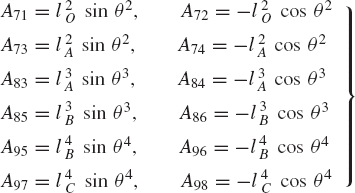
A third equation can be obtained by examining the system shown in Fig. 14. By taking the moments about point C, the following equation can be obtained:
where
By using the first two moment equations about A and B (Eqs. 79 and 81), the third equation (Eq. 82) reduces to
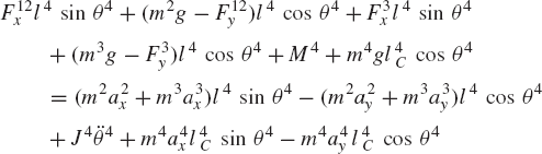
Equations 79, 81, and 84 can be solved for the three unknowns: the two reactions F12x and F12y and the external moment M4. Using a similar procedure, another set of three equations in terms of F23x, F23y, and M4, or in terms of F34x, F34y, and M4, or in terms of F41x, F41y, and M4 can be obtained. It is clear, however, that unlike the case of open kinematic chains the equilibrium conditions of the subsystems of closed kinematic chains will always lead to a set of equations that contain some components of the reaction forces. Obviously, these reaction forces can be eliminated by further manipulations of the resulting equations.
The source of the extra efforts required for the solution of the closed-chain equations can be understood because such a chain can be converted to an open chain by making a cut at a selected secondary joint. One can systematically derive the equations of motion of the resulting open chain and augment these equations by a set of algebraic equations that describe the connectivity conditions at the secondary joint, thereby defining the differential and algebraic equations of the closed chain. Lagrange multipliers and the augmented formulation, which is discussed in detail in Chapter 6, can be used to solve the chain differential and algebraic equations. Another alternative approach is to use further manipulations to eliminate the dependent variables using the algebraic constraint equations of the secondary joint. In the latter case, a procedure similar to the embedding technique can be employed.
In this chapter, different forms of the dynamic equations of motion were presented. These different forms were developed using elementary Newtonian mechanics. Among the forms discussed in this chapter, two forms are widely used in computational dynamics: the augmented formulation and the embedding technique. The augmented formulation leads to a relatively large system of equations expressed in terms of a redundant set of coordinates. As a result of this redundancy, the coordinates are not independent and they are related by a set of kinematic constraints. As was pointed out, the number of dependent coordinates used in the augmented formulation is equal to the number of independent constraint forces. By using the equations of motion and the constraint equations, a number of equations equal to the number of unknown variables can be obtained. The augmented formulation leads to a sparse matrix structure and is used as the basis for developing many of the general-purpose multibody computer programs. Its drawbacks are the increase in problem dimensionality and the need for using a more elaborate numerical algorithm to solve the resulting system of differential and algebraic equations, as discussed in Chapter 6. A systematic construction of the equations of motion of multibody systems using the augmented formulation is also presented in detail in Chapter 6.
In the embedding technique, the vector of the system accelerations is expressed in terms of independent accelerations using the velocity transformation matrix. This kinematic relationship is used to obtain a minimum set of differential equations expressed in terms of the independent accelerations only. It was demonstrated that the use of the embedding technique leads to elimination of the constraint forces. In the following chapter we discuss the principle of virtual work, which can be used to systematically eliminate the constraint forces and obtain a minimum set of differential equations of motion.
Discuss the relationship between the number of dependent coordinates used to describe the dynamics of a multibody system and the number of the constraint forces that appear in the dynamic equations.
What are the advantages and drawbacks of the augmented formulation?
Discuss the sparse matrix structure of the augmented formulation and how such a structure can be utilized in the computer implementation of this formulation.
Can you formulate the pin joint constraints of Eqs. 14 and 15 to obtain a symmetric coefficient matrix in Eq. 24?
Develop the equations of motion of the two-link robotic system shown in Fig. 8 using the augmented formulation.
Develop the equations of motion of the four-bar mechanism shown in Fig. 11 using the augmented formulation.
What are the advantages and drawbacks of the embedding technique?
What is the role of the velocity transformation matrix in the embedding technique?
Discuss the basic differences between the techniques presented in Sections 6 and 7.
Develop the equations of motion of the two-link robotic system shown in Fig. 8 using the embedding technique.
Develop the equations of motion of the four-bar mechanism shown in Fig. 11 using the embedding technique.
What are the differences between the augmented and amalgamated formulations?
What are the differences between open and closed kinematic chains when the equations of motion are formulated?