As shown in the preceding chapter, when the kinematic relationships are expressed in terms of the system degrees of freedom, the application of the principle of virtual work in dynamics leads to a number of dynamic differential equations equal to the number of the system degrees of freedom. In these equations the forces of the workless constraint are automatically eliminated. Constraint forces, however, appear in the dynamic equations if these equations are formulated in terms of a set of coordinates that are not totally independent, as discussed in Chapter 4. The number of independent constraint forces that appear in these equations is equal to the number of dependent coordinates used in the dynamic formulation.
In this chapter, the concepts and techniques, presented in Chapter 4 based on the Newtonian approach and D'Alembert's principle, are generalized using the technique of the virtual work presented in the preceding chapter. The principle of virtual work can be used to provide a proof for the existence of Lagrange multipliers when redundant coordinates are used with the augmented formulation. The virtual work principle, as demonstrated in the preceding chapter, can also be used to systematically define the velocity transformation required in the case of the embedding technique. In this chapter, the general augmented form of the equations of motion of multibody systems that consist of interconnected bodies is developed using the absolute Cartesian coordinates. The use of these coordinates allows treating the bodies as free when the unknown constraint forces are added to the other known applied forces. The generalized inertia and applied forces associated with the redundant Cartesian coordinates are first defined using the virtual work. Using the principle of virtual work, it is shown that the Newton-Euler formulation of the equations of motion can be obtained as a special case of a more general form of the equations of motion. In the case of the Newton-Euler formulation, the reference point of the body is assumed to be the body center of mass. Using this assumption, the inertia coupling between the translation and rotation of the body can be eliminated. A set of algebraic equations that describe the kinematic relationships between the redundant variables is formulated and used to systematically define the generalized constraint forces. The equations of motion of the system can then be defined in terms of the redundant coordinates and the generalized constraint forces. The computational and numerical procedures used for the computer-aided dynamic analysis of multibody systems are also discussed in this chapter, including topics such as sparse matrix techniques which are required for the efficient solution of the constrained multibody system dynamic equations. The use of the methods developed in this chapter is demonstrated using planar systems in order to emphasize the concepts and procedures presented without delving into the details of the three-dimensional motion. The analysis of the spatial systems is presented in the following chapter.
In this section, we demonstrate that the concept of equipollent systems of forces can also be applied to the inertia forces. This concept allows us to use the simple definition of the inertia forces defined at the center of mass of the body to obtain the inertia forces associated with the coordinates of an arbitrary point. It is important to understand how to apply the principle of virtual work to obtain different forms of the equations of motion, and to understand how the choice of the body reference point affects the forms of the inertia matrix and forces. Being able to use the virtual work principle effectively allows for the systematic formulation of the dynamic equations of motion of more complex systems as in the case when the bodies deform and the assumption of rigidity is no longer valid.
If the reference point Oi of the rigid body is selected to be its center of mass, the inertia force and the inertia moment are
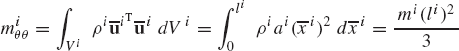
where mi is the mass of the rigid body i, Ji is the polar mass moment of inertia of the body about an axis passing through its mass center, Rix and Riy are the coordinates of the reference point, and θi is the angular orientation of the body. The mass moment of inertia Ji is defined as
where ρi and Vi are, respectively, the mass density and volume of the rigid body i, and
The virtual work of the inertia force Fii and the inertia moment Mi is given by
where Ri = [Rix Riy]T.
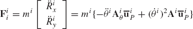
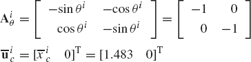
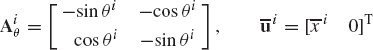
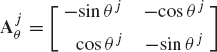
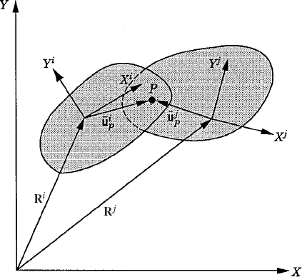
The inertia forces and moment acting at the center of mass may be replaced by an equipollent system of inertia forces and moments acting at another point on the body. The original and the equivalent systems must do the same work and accordingly, the selection of the reference point is a matter of preference or convenience. To demonstrate this fact, let Pi be an arbitrary point on the rigid body. As shown in Fig. 1, the position vector of point Pi in terms of the coordinates of the reference point is
where Ai is the transformation matrix from the body coordinate system to the global coordinate system, and
or equivalently
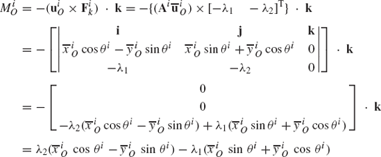
Substituting Eq. 6 into Eq. 3 leads to
One can show that
where
This equation states that the system of inertia forces and moments acting at the reference point (center of mass) is equipollent to another system, defined at the arbitrary point Pi, which consists of the force Fii and the moment Mii−(uiP×Fii).k. This fact is the familiar result obtained for the equivalence of systems of applied forces.
The parallel axis theorem can be obtained from Eq. 9 as a special case. To demonstrate this, we consider the special case where point Pi is a fixed point. In this special case, δriP = 0, and Eq. 9 reduces to
where
Using this equation, one can verify that
where
where JiP is the mass moment of inertia about an axis passing through point Pi and is defined as
This equation is the parallel axis theorem, which states that the mass moment of inertia defined with respect to an arbitrary point Pi on the rigid body is equal to the mass moment of inertia defined with respect to the center of mass plus the product of the mass and the square of the distance between point Pi and the center of mass. This familiar result was obtained in this section using the general expression of the virtual work of the inertia forces as defined by Eq. 9. It is important to emphasize, however, that if point Pi is not a fixed point, the general expression of Eq. 9 must be used in order to define the equivalent system of inertia forces at Pi. In this case, the resulting system consists of an inertia force vector as well as a moment, as demonstrated by the following example.
Example 6.1
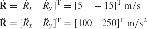
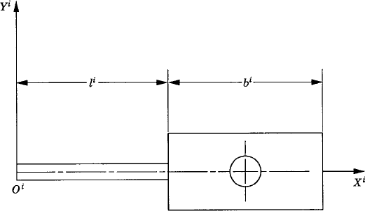
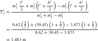
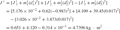
Figure 2 shows a composite body i that consists of a slender rod, a rectangular prism, and a removed round disk. The length of the rod is li = 1 m, its mass is mi1 = 0.62 kg, and its mass moment of inertia about its center of mass is Ji1 = 5.167×10⁻² kg. wwm2. The length of the rectangular prism is bi = 1 m, its mass before the removal of the disk is mi2 = 39.45 kg, and its mass moment of inertia about its center of mass is Ji2 = 4.109 kg. m2. The diameter of the removed round disk is Di = 0.25 m, its mass is mi3 = 3.873 kg, and its mass moment of inertia about its center of mass is Ji3 = 3.026 × 10⁻² kg · m2. Using the parallel axis theorem, determine the mass moment of inertia of the composite body about the body center of mass. If the absolute acceleration of the center of mass of the body at a given instant of time is defined by the vector aic = [100 −45]T m/s2, and the angular acceleration of the body is 150 rad/s2, determine the generalized inertia forces associated with the coordinates of the reference point Oi and the orientation of the body θi. Assume that θi = π/2.
Solution. The location of the center of mass of the composite body in the coordinate system shown in the figure is given by
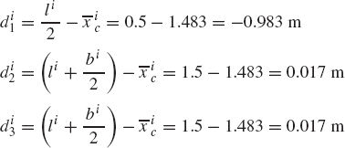
One can then define the location of the center of mass of the rod, the rectangular prism, and the removed round disk, from the center of mass of the composite system, respectively, as
Using the parallel axis theorem, the mass moment of inertia of the composite system about its center of mass can be obtained as
The parallel axis theorem can also be used to determine the mass moment of inertia about the reference point Oi as
where mi is the total mass of the composite body defined as
It follows that
The virtual work of the inertia forces is
where ric is the global position vector of the center of mass. This vector can be expressed in terms of the reference coordinates as
where Ri is the global position vector of the reference point, and
which defines the generalized inertia force associated with the translation of the body reference as
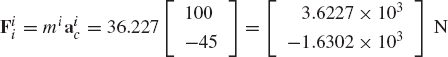
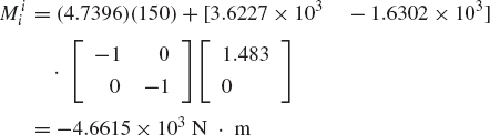
and the generalized inertia moment as
Thus
Note that
In this section, an expression for the kinetic energy for the rigid body i is defined and used to develop the general form of the mass matrix of a rigid body that undergoes an arbitrary large displacement. The effect of the selection of the reference point on the form of the kinetic energy and the mass matrix of the rigid body is also examined.
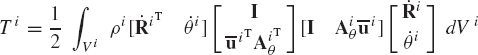
The kinetic energy of the rigid body i is defined as
where ρi and Vi are, respectively, the mass density and volume of the body, and ri is the global position vector of an arbitrary point on the rigid body. The vector ri can be expressed in terms of the coordinates Ri of the reference point and the angle of rotation θi of the body as
where Ai is the planar transformation matrix, and
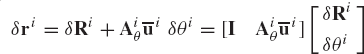
This equation can be written in a matrix form as

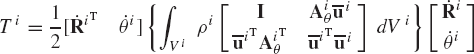
where I is the 2×2 identity matrix. Substituting Eq. 18 into Eq. 15, one obtains
which upon carrying out the matrix multiplication and utilizing the fact that AiθT Aiθ = I, one obtains
which can be written as
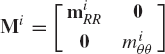
where qi and Mi are, respectively, the vector of coordinates and mass matrix of the rigid body i given by
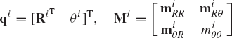
in which
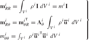
and mi is the total mass of the body. Note that miθθ is a scalar that defines the body mass moment of inertia with respect to an axis passing through the reference point of the body. The matrix miRθ and its transpose miθR represent the inertia coupling between the translation of the reference point and the rotation of the body.
Example 6.2
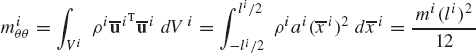
In order to demonstrate the use of Eqs. 22 and 23, we consider the case of a uniform slender rod that has mass density ρi, cross-sectional area ai, and length li. We assume that the reference point is selected to be one of the endpoints at which
and
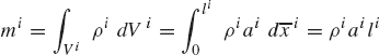
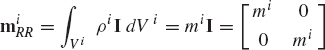
where Vi is the volume, and mi is the total mass of the rod. The matrix miRR can be evaluated as
The matrix miRθ, which represents the inertia coupling between the translation and rotation of the rod, can be written as
in which
It follows that
The mass moment of inertia of the rod defined with respect to an axis passing through the reference point is given by
Therefore, the mass matrix of the rod is given by

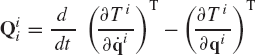
The general expression of the kinetic energy obtained in Eqs. 21 can be used to define the generalized inertia forces of the rigid body i using Lagrange's equation. In this case, one has
Another elegant way for defining the generalized inertia forces associated with the absolute coordinates is to use the virtual work. Recall that the virtual work of the inertia forces of the rigid body i is defined as
where ri is the global position vector of an arbitrary point on the rigid body as defined by Eq. 16. It follows that
This equation can be written as
where
Using Eq. 18, the absolute velocity and acceleration vectors of the arbitrary point can be written as
in which
Substituting Eqs. 27 and 29 into Eq. 25, one obtains
Note that the symmetric mass matrix of Eqs. 22 is
Equation 31 can then be written as
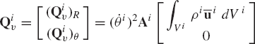
where Qiv is the vector of centrifugal inertia forces defined as
Substituting Eqs. 28 and 30 into Eq. 34, one obtains
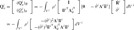
The product AiθT Ai is a skew-symmetric matrix defined as
and as a consequence
For the simple rod discussed in Example 2 one can show that the vector of centrifugal inertia forces is
A special case of the foregoing development is the case in which the reference point is selected to be the center of mass of the body. This is the case of a centroidal body coordinate system.
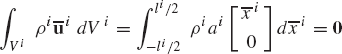
The integral in the second equation of Eqs. 23 represents the moment of mass of the body. If the reference point is chosen to be the center of mass, this integral is identically zero; that is,
and, as a consequence, the matrices miRθ and miθR defined by Eqs. 23 are identically equal to zero. In this special case, the mass matrix Mi of the body reduces to
and the kinetic energy of the body can be written as
In this special case, there is no coupling between the translation and rotation of the body in the mass matrix. Furthermore, the vector of centrifugal inertia forces is identically equal to zero, that is
Thus, in the case of a centroidal body coordinate system, the mass matrix of a rigid body in planar motion is diagonal, the vector of centrifugal inertia forces vanishes, and the kinetic energy of the rigid body consists of two terms; one is due to the translation of the center of mass and the other is due to the planar rigid body rotation.
Example 6.3
Consider the slender rod of Example 2. The rod is assumed to have mass density ρi, cross-sectional area ai, and length li. We consider the case where the reference point is selected to be the center of mass of the rod. In this case, one has
which implies that
The matrix miRR is

The mass moment of inertia miθθ is given by
The mass matrix of the rod can then be written as
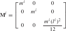
Comparing the results obtained in this example and the results of Example 2, we see that the mass matrix in the case of a centroidal body coordinate system is diagonal, as compared to the nondiagonal mass matrix obtained in the preceding example. Furthermore, the mass moment of inertia obtained when the reference point is selected to be at one of the endpoints of the rod is equal to the mass moment of inertia defined with respect to the center of mass plus mi(li/2)2.
The equations of motion of the rigid body are developed in this section in terms of the absolute Cartesian coordinates that represent the translation of the reference point of the body as well as its orientation with respect to the global inertial frame of reference. This representation will prove useful in developing general-purpose computer algorithms for the dynamic analysis of interconnected sets of rigid bodies, since practically speaking, there is no limitation on the number of bodies or the types of forces and constraints that can be introduced to this formulation.
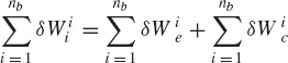
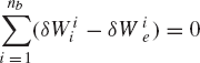
In the preceding chapter, it was shown that the conditions for the dynamic equilibrium for the rigid body i can be developed using the principle of virtual work as
where δWii is the virtual work of the inertia forces, δWie is the virtual work of the externally applied forces, and δWic is the virtual work of the constraint forces. The virtual work of the externally applied forces can be expressed in terms of the vector of generalized coordinates as
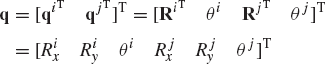
where Qie is the vector of generalized forces, and qi is the vector of generalized coordinates of the rigid body i. Using the Cartesian coordinates, the vector qi is given by
where Ri is the position vector of the reference point, and θi is the angular orientation of the body.
One can also write the virtual work of the joint constraint forces acting on the rigid body i as
where Qic is the vector of the generalized constraint forces associated with the body generalized coordinates.
The virtual work of the inertia forces can be obtained using the development of the preceding section as
where Mi is the symmetric mass matrix of the body defined in Eqs. 22 or equivalently by Eq. 32, and Qiv is the vector of centrifugal forces defined by Eq. 37.
Substituting Eqs. 43, 45 and 46 into Eq. 42, one obtains
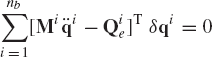
which, upon utilizing the fact that the mass matrix is symmetric, leads to
Since the constraint forces, as result of the connection of this body with other bodies in the system, are included in this equation and represented by the vector Qic, the elements of the vector qi can be treated as independent. Consequently, Eq. 48 leads to
which can be rewritten according to the coordinate partitioning of Eq. 44 as
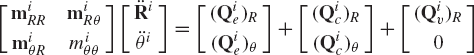
Equation 49, or its equivalent form of Eq. 50, represents the dynamic equations of motion of the rigid body i, developed using an arbitrary reference point.
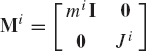
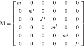
If the reference point is selected to be the center of mass of the body, one has miRθ = miθRT = 0 and Qiv = 0. In this case, Eq. 49 reduces to
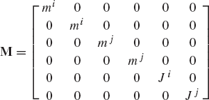
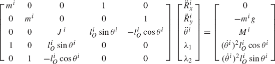
which can be written in a more explicit form as
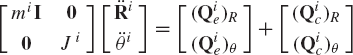
where mi is the mass of the body, and Ji is its mass moment of inertia about an axis passing through the center of mass. Clearly, Eq. 52 is the same as the fundamental Newton and Euler equations that govern the motion of the rigid bodies. These equations are obtained, however, as a special case of the general form represented by Eq. 50.
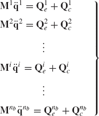
It was shown in the preceding section that affixing the origin of the body coordinate system to the body center of mass leads to a significant simplification in the resulting dynamic equations. Therefore, without any loss of generality, we consider the case of a centroidal body reference where the origin of the body coordinate system is rigidly attached to the body center of mass. In this case, the mass matrix is diagonal and the vector of centrifugal forces is identically equal to zero. By using Eq. 51, the equations of motion of a multibody system consisting of nb interconnected bodies are given by
which can also be written as
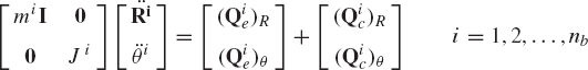
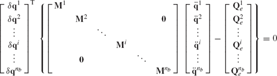
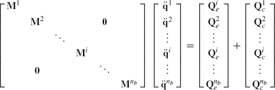
where all the scalars, vectors, and matrices that appear in Eq. 53 and 54 are the same as defined in the preceding section. The number of scalar equations given by the matrix equation of Eq. 53 or Eq. 54 is 3 × nb. These equations can be combined into one matrix equation given by

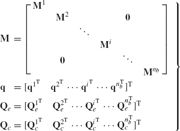
which can be written as
where M is the system mass matrix, q is the total vector of system generalized coordinates, Qe is the vector of system generalized external forces, and Qc is the vector of the system generalized constraint forces. The mass matrix M and the vectors q, Qe, and Qc are
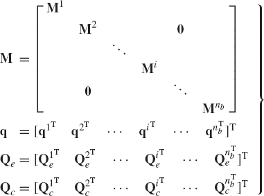
Note that the equations of motion of the multibody system given by Eq. 56 contain the generalized constraint forces, since these equations are not expressed in terms of the system degrees of freedom.
Example 6.4
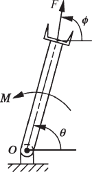
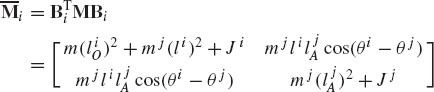
Figure 3a shows a two link planar manipulator. The origins of the body coordinate systems are assumed to be rigidly attached to the centers of mass of the links. Let mi and Ji, and mj and Jj be, respectively, the mass and mass moment of inertia of links i and j, and Mi and Mj be, respectively, the external torque applied to links i and j. Obtain the differential equations of motion of the system in terms of the absolute coordinates. Neglect the effect of gravity.
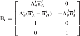
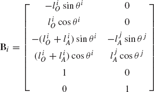
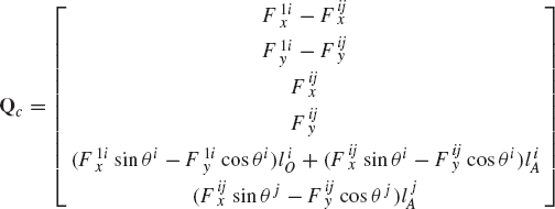
Solution. The virtual work of the reaction forces acting on link i can be expressed as
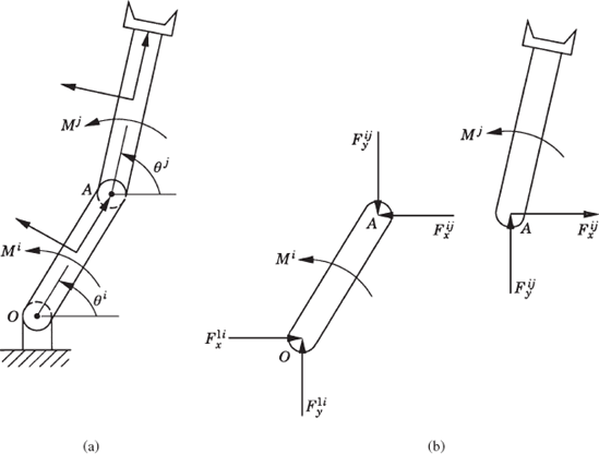
where F1ix, F1iy, Fijx, and Fijy are the reaction forces acting on link i as shown in Fig. 3b, and δriO and δriA can be expressed in terms of the absolute coordinates of link i as
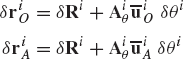
where

and liO and liA are, respectively, the distances of points O and A from the center of mass of link i. The virtual work of the reaction forces of link i is
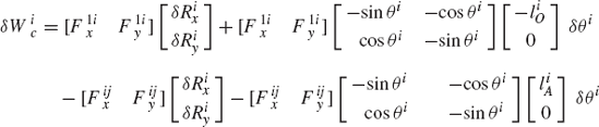
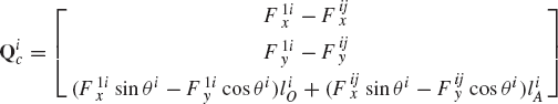
This equation leads to
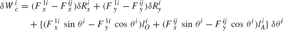
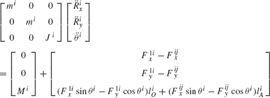
from which the vector of generalized reactions Qic associated with the absolute coordinates of link i can be expressed as
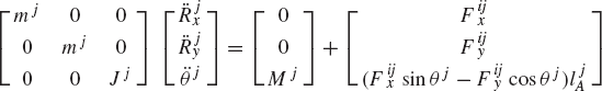
Using Eq. 54, the equation of motion of link i can be written as
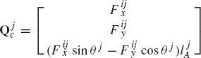
Similarly, the virtual work of the generalized reactions acting on link j is
where
in which
and
where ljA is the distance of point A from the center of mass of link j. It follows that

from which the vector of joint reaction forces Qjc associated with the absolute coordinates of link j can be defined as
The equations of motion of link j are
The system equations of motion can be defined as
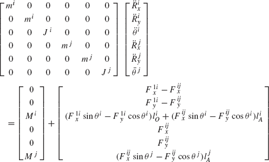
These are six scalar equations in 10 unknowns
since δriO = 0, and δriA = δrjA.
The equations of motion obtained for the multibody system in the preceding section and given by Eq. 56 contain the generalized constraint forces due mainly to the fact that these equations are formulated using a redundant set of coordinates. It is important, however, to point out that the force of constraints can be eliminated from the dynamic formulation if the redundant coordinates are expressed in terms of the independent coordinates, as discussed in the preceding chapter. To illustrate the use of such a procedure, Eq. 42, which is a statement of the principle of virtual work for body i, is used. If the multibody system consists of nb interconnected bodies, Eq. 42 leads to
As demonstrated in the preceding chapter,
Substituting Eqs. 43 and 46 into this equation, and keeping in mind that the origin of the body i coordinate system is rigidly attached to the body center of mass, that is Qiv = 0, one obtains
which can be written in a matrix form as

This equation can also be written as
or
where M is the system mass matrix, q is the vector of system absolute coordinates, and Qe is the vector of system generalized forces associated with the absolute coordinates. The matrix M and the vectors q and Qe are defined in the preceding section.
Equation 63 is a scalar equation that does not contain the constraint forces. The coefficient vector
where C = [C1(q, t) C2(q, t)...Cnc(q, t)]T is the vector of linearly independent constraint equations, and nc is the number of constraint functions.
For a virtual change in the system coordinates, Eq. 64 yields
where Cq is the constraint Jacobian matrix defined as
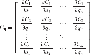
in which q = [q1 q2...qn]T is the n-dimensional vector of system coordinates.
Because of the kinematic constraints of Eq. 64, the components of the vector q are not independent. One, therefore, may write the vector q in the following partitioned form:
where qd is the nc-dimensional vector of dependent coordinates and qi is the vector of independent coordinates, which has the dimension (n−nc). According to the coordinate partitioning of Eq. 67, Eq. 65 can be written as
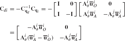
where the vector qd is selected such that the matrix Cqd is nonsingular. This choice of the matrix Cqd is always possible since the constraint equations are assumed to be linearly independent. Equation 68 can then be used, as described in the preceding chapter, to write the virtual changes of the dependent coordinates in terms of the virtual changes of the independent ones as
in which
The virtual changes in the total vector of system coordinates can be written in terms of the virtual changes of the independent coordinates using Eq. 70 as
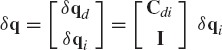
which can be written as
where
Equations 63 and 73 can be used to obtain a minimum number of differential equations expressed in terms of the independent coordinates. In order to demonstrate this, Eq. 73 is substituted into Eq. 63, leading to
Since the components of the vector δqi are independent, their coefficients in Eq. 75 must be equal to zero. This leads to
This is a system of n−nc differential equations that can be expressed in terms of the independent accelerations. For instance, by differentiating Eq. 64 once and twice with respect to time, one obtains

where subscript t indicates a partial differentiation with respect to time. By using the coordinate partitioning of Eq. 67, the second equation in Eq. 77 can be written as
where
Equation 78 can then be used to write the total vector of system accelerations in terms of the independent ones as
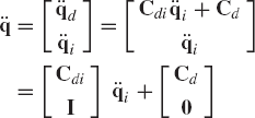
which upon using Eq. 74 leads to
where
Using Eqs. 76 and 81, one obtains
which can be written as
where
For a given system of forces, Eq. 84 can be solved for the independent accelerations as follows:
For a well-posed problem with linearly independent constraint equations, the inverse of the matrix
It is important to mention that Eq. 84 can be obtained directly from Eq. 56 by using Eq. 81. The transformation of Eq. 81 automatically eliminates the constraint force vector Qc of Eq. 56. Substituting Eq. 81 into Eq. 56, one obtains
Premultiplying this equation by BTi, one obtains
Since this equation is expressed in terms of the independent accelerations, one must have
which implies that the columns of the matrix Bi are orthogonal to the constraint force vector Qc. Consequently, the system differential equation reduces to
The matrices and vectors that appear in this equation are exactly the same as those of Eq. 83 which was used to define Eq. 84.
Example 6.5
For the two-link manipulator of Example 4, the revolute joint constraints at points O and A can be written as
which can be expressed in terms of the absolute coordinates of the two links as
These are four scalar constraint equations in which
The vector of constraints C(q, t) can then be written as
where
It follows that
Since the system has two degrees of freedom, we may select θi and θj to be the independent coordinates, that is
According to this coordinate partitioning, the preceding equation can be rewritten as
where the Jacobian matrices Cq, Cqd and Cqi can be recognized as

The matrix Cqd is nonsingular and its inverse is
The matrix Cdi of Eq. 71 can then be defined as
The matrix Cdi is a 4 × 2 matrix since the system has four dependent coordinates and two independent coordinates. The virtual change of the system coordinates can be expressed in terms of the virtual changes of the independent coordinates using Eq. 73, where in this example, the matrix Bi of Eq. 74 is given by
This is a 6 × 2 matrix since the system has six coordinates and only two of them are independent. The matrix Bi can be written more explicitly as
The mass matrix of the system, which was derived in Example 4, can be rearranged according to the partitioning of the coordinates as dependent and independent. This yields
It follows that
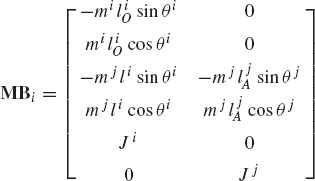
where li = liO + liA is the length of link i. The mass matrix associated with the independent coordinates can be evaluated using Eq. 85 as
which is a 2 × 2 symmetric matrix, since the system has two degrees of freedom.
The constraint force vector Qc of the system discussed in this example was defined in Example 4. If the components of this vector are rearranged according to the partitioning of the coordinates as dependent and independent, one obtains
It is easy to verify that
In the computer analysis of large-scale mechanical systems, numerical methods are often used to identify the system-dependent and system-independent coordinates. Based on the numerical structure of the constraint Jacobian matrix, an optimum set of independent coordinates can be identified. Recall that for a dynamically driven system, the Jacobian matrix is an nc × n nonsquare matrix, where nc is the number of constraint equations and n is the total number of the system coordinates. If the constraints are linearly independent, the Jacobian matrix has a full row rank, and Gaussian elimination can be used to identify a nonsingular nc × nc sub-Jacobian. For instance, applying the Gaussian elimination method with complete or full pivoting on the constraint Jacobian matrix of Eq. 66 and assuming that no zero pivots are encountered, Eq. 65, after nc steps, can be written in the following form:
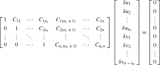
In the case of full pivoting, elementary column operations are used and the elements of the vector δq are reordered accordingly. Hence, the vectors δu = [δu1 δu2...δunc]T and δv = [δv1 δv2...δvn − nc]T contain elements of the vector δq, which are reordered as the result of the elementary column operations. The preceding equation can be written in a partitioned form as
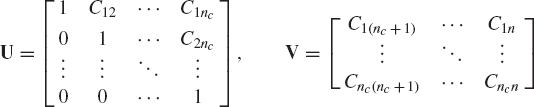
The matrix U is an upper-triangular matrix with all the diagonal elements equal to one. Because this matrix is nonsingular, the vector δu can be expressed in terms of the components of the vector δv. The elements of the vector δv can then be recognized as the independent coordinates and the elements of the vector δu are recognized as the dependent coordinates, that is,
The Gaussian elimination method can also be used to detect redundant constraints. If such redundant constraints exist, the constraint equations are no longer independent and the constraint Jacobian matrix does not have a full row rank. In this case, the Gaussian elimination procedure leads to zero rows, and the number of these zero rows is equal to the number of the dependent constraint equations which is the same as the row-rank deficiency of the constraint Jacobian matrix. The redundant constraints must be eliminated in order to determine a set of linearly independent constraint equations that yield a Jacobian matrix that has a full row rank.
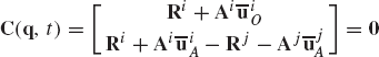
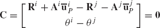
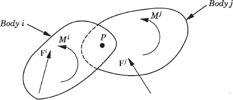
The embedding technique that leads to a minimum set of strongly coupled equations has several computational disadvantages. It requires finding the inverse of the sub-Jacobian matrix associated with the dependent coordinates and it also leads to a dense and highly nonlinear generalized mass matrix. In this section, some basic concepts in the force analysis of constrained systems of rigid bodies are discussed. These concepts, which are fundamental and are widely used in classical and computational mechanics, will allow us to obtain a system of loosely coupled dynamic equations in which the coefficient matrix is sparse and symmetric. The solution of this system of equations defines the accelerations and a set of multipliers that can be used to define the constraint forces. In order to introduce these multipliers, we first consider the simple system shown in Fig. 4. The system consists of two rigid bodies, body i and body j, which are rigidly connected at point P. The constraint equations for this system can be expressed in terms of the Cartesian coordinates as
where Ri and Rj are, respectively, the global position vectors of the origins of the coordinate systems of bodies i and j, Ai and Aj are, respectively, the transformation matrices from the coordinate systems of body i and body j to the global coordinate system,
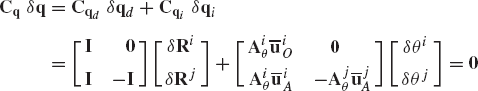
Equation 95 can be written as
where C is the vector of constraint equations defined as
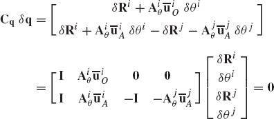
The Jacobian matrix of these constraint equations can be written in a partitioned form as
where
where I is the 2 × 2 identity matrix and Aiθ and Ajθ are, respectively, the partial derivatives of the transformation matrices Ai and Aj with respect to the rotational coordinates θi and θj.
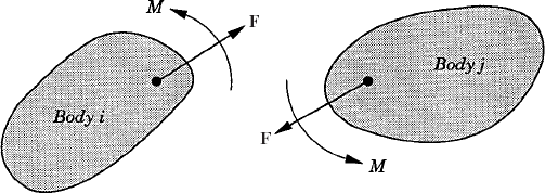
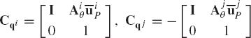
Figure 5 shows the actual reaction forces acting on bodies i and j of Fig. 4 as a result of the rigid connection between the two bodies. Let λ be the vector
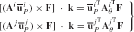
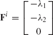
The reaction forces acting on body i and body j, which are equal in magnitude and opposite in direction, can be expressed, respectively, in a vector form as
The systems of the actual reaction forces of Eq. 101 are equipollent to other systems of generalized reaction forces defined at the origins of the coordinate systems of the two bodies and given by

Equation 102 is the result of the simple fact that a force F acting at a point P is equipollent to a system of forces that consists of the same force acting at another point O plus a moment defined as the cross product between the position vector of P with respect to O and the force vector F.
Recall that
Using these identities and Eq. 102, one obtains

which can be written using matrix notation as
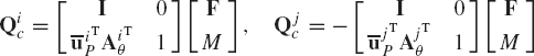
Comparing the matrices in these equations with the Jacobian matrices of Eq. 99, one concludes that the generalized reactions can be expressed in this example in terms of the actual reactions as
Each equation of Eq. 106 contains three force components; two force components associated with the translation of the reference point and one component associated with the rotation of the body. Equation 106 implies that the generalized reaction forces as the result of the rigid connection between bodies i and j can be expressed in terms of the Jacobian matrices of the kinematic constraint equations. In this example, the vector λ was found to be the negative of the vector that contains the reaction force and moment. The vector λ, whose dimension is equal to the number of constraint equations, is called the vector of Lagrange multipliers. While the form of Eq. 106 is valid for all types of constraints, the vector of Lagrange multipliers may not, in some applications, take the simple form of Eq. 100.
Example 6.6
Find the generalized reaction forces associated with the Cartesian coordinates of two bodies i and j connected by a revolute joint in terms of Lagrange multipliers.
Solution. The revolute joint between two bodies i and j allows only relative rotation. The constraint equations for this joint are
where
which can be written as
in which
The generalized constraint reactions of the revolute joint associated with the translation of the reference points and the rotations of the bodies i and j are
which can be written explicitly as
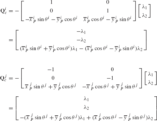
where
Example 6.7
A link in a mechanism is assumed to be fixed if it is subjected to the ground constraints, which do not allow the translational and rotational displacements of the link. These ground constraints for link i are given by
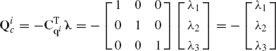
where C1 and C2 are, respectively, a constant vector and a constant scalar. The Jacobian matrix of the ground constraints is

The generalized reactions as the result of imposing the ground constraints are
A body in a multibody system may be connected to other bodies by several joints. For example, in multibody vehicle systems the chassis of the vehicle is connected to the suspension elements by different types of joints. If a body in the mechanical system is connected with other bodies by more than one joint, one can use the procedure previously described in this section to define the contribution of each joint to the generalized reaction forces. For example, let body i be connected to other bodies in the system by ni joints. The constraint equations that describe these joints can be expressed in vector forms as
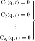
where

where λk is the vector of Lagrange multipliers associated with the vector of constraints Ck. The resultant generalized reaction forces due to all the constraints of Eq. 107 can be written as
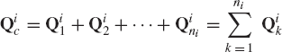
which upon using Eq. 108, yields
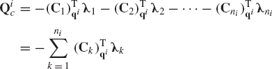
Equation 110 can also be written in a matrix form as
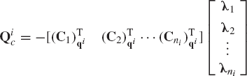
It is clear that there will be no contribution from other joints that do not involve body i since the constraint equations that describe these joints are not explicit functions of the coordinates of body i. Equation 111 can then be written in a more general form as
where C is the total vector of constraint equations of the system, and λ is the vector of the system Lagrange multipliers. Constraints which are not explicit functions of the coordinates of body i define zero rows in the Jacobian matrix Ciq of Eq. 112.
Equation 112 can be used to define the total vector of the system-generalized reactions. If the system consists of nb bodies, one has
which upon using Eq. 112, leads to
By factoring out the vector of Lagrange multipliers λ and keeping in mind that
where Cq is the constraint Jacobian matrix of the system, Eq. 114 can be written as
Since each joint is formulated in terms of the coordinates of the two bodies connected by this joint, the Jacobian matrix Cq in a large-scale constrained mechanical system is a sparse matrix, which has a large number of zero entries.
Example 6.8
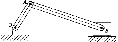
In order to demonstrate the use of Eq. 116, the slider crank mechanism shown in Fig. 6 is considered. The configuration of this mechanism can be identified using 12 Cartesian coordinates. There are, however, 11 constraint equations that describe the joints in the system. These constraint equations are the three ground constraints, the two revolute joint constraints at O, the two revolute joint constraints at A, the two revolute joint constraints at B, and the two constraints that allow only the translation of the slider block in the horizontal direction. The Jacobian matrix of the constraint equations of this mechanism was developed in Chapter 3 and is given by
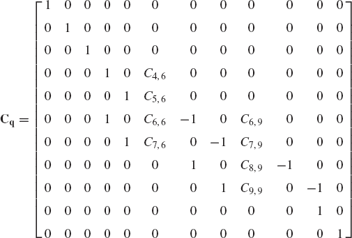
where

The vector of system generalized reaction forces is
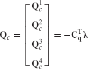
where
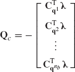
The vector Qc is given explicitly in terms of Lagrange multipliers by

The use of the generalized coordinate partitioning of the constraint Jacobian matrix to develop a minimum number of differential equations that govern the motion of the multibody system was demonstrated in Section 5. These equations are expressed in terms of the independent accelerations and, therefore, the constraint forces are automatically eliminated. An alternative approach for formulating the dynamic equations of the multibody systems is to use redundant coordinates which are related by the virtue of the kinematic constraints. This approach, in which the constraint forces appear in the final form of the equations of motion, leads to a larger system of loosely coupled equations which can be solved using sparse matrix techniques.
In this section, we discuss the augmented formulation in which the kinematic constraint equations are adjoined to the systems differential equations using the vector of Lagrange multipliers. This approach leads to a system of algebraic equations with a symmetric positive-definite coefficient matrix. This system can be solved for the accelerations and Lagrange multipliers. Lagrange multipliers can be used to determine the generalized reactions as discussed in the preceding section, while the accelerations can be integrated in order to determine the system coordinates and velocities.
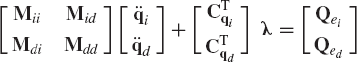
In terms of the absolute Cartesian coordinates, the motion of a rigid body i in the multibody system is governed by Eq. 51, which is repeated here as
where Mi is the mass matrix of the rigid body i,
where mi is the mass of the body, and Ji is the mass moment of inertia defined with respect to the body center of mass.
If the system consists of nb interconnected bodies, a matrix equation similar to Eq. 117 can be developed for each body in the system. This leads to
These equations can be combined in one matrix equation as
which can be written as
where
in which M is the system mass matrix, q is the total vector of system-generalized coordinates, Qe is the vector of system-generalized external forces, and Qc is the vector of the system-generalized constraint forces. It was shown in the preceding section that the vector Qc of the system-generalized constraint forces can be written in terms of the system constraint Jacobian matrix and the vector of Lagrange multipliers as
where Cq is the constraint Jacobian matrix, λ is the nc-dimensional vector of Lagrange multipliers, and nc is the number of constraint equations. Substituting Eq. 123 into Eq. 121, one obtains
These are n second-order differential equations of motion, where n is total number of system coordinates.
In the preceding section, we used a simple example to introduce the technique of Lagrange multipliers. Before we start our discussion on the solution of the equations of motion, it may be helpful to provide the general theoretical derivation of Eq. 124 in order to demonstrate the generality of the technique of Lagrange multipliers. We make use of Eqs. 63 and 65, which are given, respectively, by
and
Since the vector Cq δq is equal to zero from the second equation, the scalar product of this vector with any other vector is also equal to zero. Hence, the second equation yields
for an arbitrary vector λ, which has a dimension equal to the number of the constraint equations. When this equation is added to Eq. 125, one obtains
The coefficients of the elements of the vector δq in this equation cannot be set equal to zero because the coordinates are not independent. Using the coordinate partitioning of Eq. 67, the preceding equation yields

where the subscripts i and d refer, respectively, to independent and dependent coordinates. It follows that
and
As previously pointed out, the independent coordinates can be selected such that the matrix CTqd is a square nonsingular matrix. The vector of Lagrange multipliers can then be selected to be the unique solution of the following system of algebraic equations:
This choice of Lagrange multipliers guarantees that the coefficients of the elements of the vector δqd in Eq. 131 are equal to zero. Furthermore, since in Eq. 130 the elements of the vector δqi are independent, one has
Combining the preceding two equations, one obtains
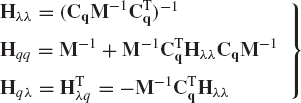
which leads to the general form of Eq. 124,
If the vector of generalized external forces Qe is known, the unknowns in Eq. 124 are the vector of accelerations
which upon differentiation once and twice with respect to time, one obtains
where the subscript t denotes partial differentiation with respect to time and Qd is a vector that absorbs first derivatives in the coordinates and is given by
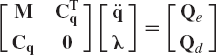
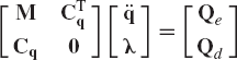
Equation 124 can be combined with the second equation of Eq. 136 in one matrix equation as
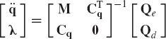
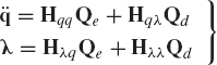
The vectors of accelerations and Lagrange multipliers can be obtained by solving Eq. 138 as
By direct matrix multiplication, one can verify that
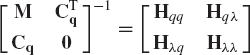
where
Substituting Eq. 140 into Eq. 139 and carrying out the matrix multiplication, one obtains
For a given set of initial conditions, the vector
It is important to emphasize at this point that due to the approximations involved in the direct numerical integration, the resulting coordinates and velocities are not exact. One, therefore, expects that the constraints of Eq. 135 will be violated with a degree depending on the accuracy of the numerical integration method used. With the accumulation of the errors in some applications, the violation in the constraints of Eq. 135 may not be acceptable. In order to circumvent this difficulty, Wehage (1980) proposed a coordinate partitioning technique in which the independent accelerations are identified and integrated forward in time using a direct numerical integration method, thus defining the independent coordinates and velocities. By knowing the independent coordinates as a result of the direct numerical integration, Eq. 135 which can be considered as nc nonlinear algebraic constraint equations in the nc-dependent coordinates is then used to determine the dependent coordinates using a Newton-Raphson algorithm. Having also determined the independent velocities as the result of the numerical integration, the first equation in Eq. 136 can be used to determine the dependent velocities by partitioning the constraint Jacobian matrix, and rewriting this equation in the following form:
where qd and qi are, respectively, the vectors of dependent and independent coordinates that are selected in such a manner that Cqd is nonsingular. It follows that
This equation defines the dependent velocities. Having determined both dependent and independent coordinates and velocities, Eq. 138 can be constructed and solved for the accelerations in order to advance the numerical integration.
Example 6.9
Figure 7 shows a two-body system that consists of body i and body j which are connected by a revolute joint at point P. In this case, the system mass matrix M is
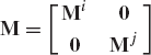
where
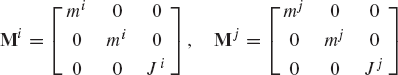
Therefore, the mass matrix M is
The Jacobian matrix of the revolute joint is
where
It can also be shown that the vector Qd of Eq. 137 is
Equation 138 for this system can be written as
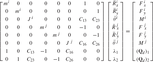
where Fi = [Fix Fiy]T and Fj = [Fjx Fjy]T are, respectively, the vectors of forces acting at the center of masses of bodies i and j, and Mi and Mj are the moments acting, respectively, on body i and body j.
The solution of Eq. 138 presented in the preceding section defines the vector of Lagrange multipliers which can be used in Eq. 123 to determine the vector of generalized constraint forces associated with the translation of the center of mass and the rotation of the body. While these generalized forces may not be the actual reaction forces of the joint, the generalized and actual constraint forces represent two equipollent systems of forces. This fact will be used to determine the actual joint forces in terms of the generalized constraint forces which are assumed, in the following discussion, to be known from the analytical or numerical solution of Eq. 138.
For a given joint k in the multibody system, the generalized constraint forces acting on body i, which is connected by this joint, are
where Fixk, Fiyk, and Mik are the components of the vector (Qic)k which are assumed to be known, Ck is the vector of constraint equations of the joint k, and λk is the vector of Lagrange multipliers associated with these constraints.
The system of forces of Eq. 145 is equipollent to another system of forces defined on the joint surface. Let uiP be the position vector of the joint definition point with respect to the reference point. A system equipollent to the system of Eq. 145 can be obtained as
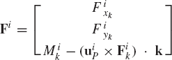
where Fik = [Fixk Fiyk]T, and k is a unit vector along the axis of rotation. Equation 146 defines the system of reaction forces at the joint.
Example 6.10
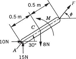
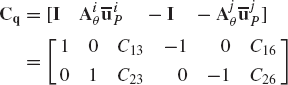
The constraint equations of the revolute joint of the pendulum shown in Fig. 8 are
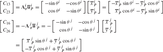
and the Jacobian matrix of the constraints are
where

The generalized reaction forces can be expressed in terms of Lagrange multipliers as
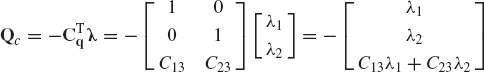
This system must be equipollent to a system of reaction forces acting at the joint. Using Eq. 146, the actual reaction forces can be written as
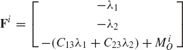
where MiO is the moment of the generalized reactions about point O and defined by the cross product
By substituting this expression into the definition of Fi and using the definition of C13 and C23, one obtains
which implies that the actual reactions at the joints are the negative of Lagrange multipliers. Furthermore, the actual moment is equal to zero, which is an expected result for the revolute joint.
A more systematic, yet equivalent, procedure for determining the reaction forces at the joint definition points is to use the virtual work. Let Fik and Mik be, respectively, the generalized constraint force and moment associated with the reference coordinates as the result of a joint k. The virtual work of the constraint force and moment can be expressed as
The global position vector of the joint definition point rik can be expressed in terms of the reference coordinates as
where Ai is the planar transformation matrix of body i, and
and
The virtual work of the constraint forces can be expressed in terms of the virtual change in the coordinates of the joint definition point as
The coefficients of δrik and δθi in this equation define the reaction force and moment at the joint definition point. In the case of a revolute joint, the coefficient of δθi in the preceding equation is identically equal to zero as demonstrated by the preceding example.
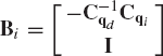
While the use of the embedding technique is not recommended as a basis for developing general-purpose multibody computer programs because of the computational overhead, it is important to understand some of the basic concepts and techniques used in classical and computational dynamics to obtain a minimum set of independent differential equations. We have previously demonstrated that if Qc is the vector of generalized constraint forces, then BTiQc = 0 (Eq. 89), where Bi is the matrix defined by Eq. 74. In the method of Lagrange multipliers, the generalized constraint forces are expressed in terms of the Jacobian matrix of the kinematic constraints as
This equation which is valid regardless of the values of Lagrange multipliers implies that the vector of generalized constraint forces
Recall that
Using this matrix, one gets
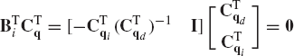
as previously stated.
The matrix Bi of Eq. 74 or 154 defines the relationship between the total vector of the system velocities and a smaller independent subset of the same velocities. There are other methods that can be used to express the system variables in terms of a more general set of independent coordinates, each of which can be a linear combination of the system coordinates. These methods can also be used to eliminate Lagrange multipliers and obtain a minimum set of independent differential equations. Among these methods are the QR decomposition and the singular value decomposition.
Assuming that the constraint equations are independent such that the constraint Jacobian matrix has a full row rank, Householder transformations can be used, as described in Chapter 2, to write the transpose of the constraint Jacobian matrix as
where Q1 and Q2 are n × nc and n × (n − nc) matrices, respectively, and R1 is an nc × nc upper-triangular matrix. It was demonstrated in Chapter 2 that the columns of the matrices Q1 and Q2 are orthogonal and
In the QR decomposition, one can select the matrix Bi, such that
With this choice of Bi, we are guaranteed that
As pointed out in Chapter 2, while Q1 and R1 in the QR decomposition are unique, the matrix Q2 in this factorization is not unique. It is, therefore, numerically difficult to preserve the directional continuity of the bases represented by the columns of the transformation Q2. Kim and Vanderploeg (1986) defined constant orthogonal matrices Q1 and Q2 at the initial configuration and used the velocity constraint relationships to iteratively update these matrices in order to preserve the directional continuity of the null space of the constraint Jacobian matrix.
The singular value decomposition of the transpose of the Jacobian matrix can be written as
where Q1 and Q2 are two orthogonal matrices whose dimensions are n × n and nc × nc, respectively, and B is an n × nc matrix that contains the singular values along its diagonal. It was shown in Chapter 2 that the preceding equation can be written in the following partitioned form:
where B1 is a diagonal matrix, and Q1d and Q1i are partitions of the matrix Q1. The columns of the matrices Q1d and Q1i are orthogonal vectors and
It is also clear that
The preceding two equations imply that
If the matrix Bi is selected such that
then
Kim and Vanderploeg (1986) pointed out that the QR decomposition is about two times more computationally expensive than the LU decomposition, while the singular value decomposition is two to ten times more expensive than the QR decomposition, depending upon the size of the constraint Jacobian matrix. The QR and the singular value decompositions can also be used to obtain an identity-generalized mass matrix associated with the independent coordinates. For example, in the planar analysis using the absolute Cartesian coordinates, the mass matrix M of Eq. 122 is a diagonal matrix whose inverse can be easily defined. Multiplying Eq. 124 by the inverse of the mass matrix, one obtains
Now, let Bi be the orthogonal velocity transformation obtained by the QR decomposition or the singular value decomposition of the matrix M−1CTq. Substituting the transformation
By now, it should be clear that there are two basic approaches for formulating the dynamic equations of multibody mechanical systems. These approaches are the embedding technique and the augmented formulation. In the embedding technique, the dynamic equations are formulated in terms of the system degrees of freedom, thereby eliminating the workless constraint forces. This approach leads to a system of linear algebraic equations in the independent accelerations. The coefficient matrix in this system of algebraic equations is the generalized mass matrix associated with the independent coordinates, and the right-hand side is the vector of externally applied and centrifugal forces which depend on the system coordinates, velocities, and possibly on time. By assuming that the mass matrix is positive definite, the inverse of this matrix can be obtained and used to express the independent accelerations in terms of the independent coordinates, velocities, and time. This procedure leads to Eq. 86,
where Gi is the vector function
In the second approach, the augmented formulation is used, leading to the dynamic equations which are expressed in terms of the dependent and independent accelerations. The nonlinear algebraic constraint equations are adjoined to the dynamic equations using the vector of Lagrange multipliers. This formulation leads to a linear system of algebraic equations in the system accelerations and Lagrange multipliers. The coefficient matrix in this system of equations (Eq. 138) depends on the system mass matrix as well as the constraint Jacobian matrix. As shown in Section 7, the solution of this system of equations defines the vector of accelerations as well as the vector of Lagrange multipliers (Eqs. 142), which can be used to evaluate the generalized reaction forces, as discussed in the preceding section. Clearly, in this case the independent accelerations can be identified and expressed in the form of Eq. 165, and consequently, the form of Eq. 165 can be obtained by using the embedding technique, or by using the augmented formulation.
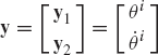
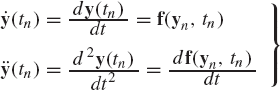
Having expressed the independent accelerations in terms of the independent coordinates, velocities, and time, one can proceed a step further in the direction of obtaining the numerical solution of the nonlinear equations of the multibody system. To this end, we define the state vector y as

The dimension of this vector is equal to twice the number of the system degrees of freedom. Differentiating Eq. 166 with respect to time and using the definition of Eq. 166, one obtains the following first-order state equations:
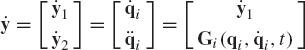
Since
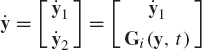
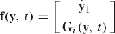
which can simply be written as
where
Equation 169 represents the state space equations of the multibody system. These equations are first-order differential equations and their number is equal to twice the number of the system degrees of freedom. Therefore, in the state space formulation, the second-order differential equations associated with the independent coordinates are replaced by a system of first-order differential equations that has a number of equations equal to twice the number of the degrees of freedom of the system.
Example 6.11
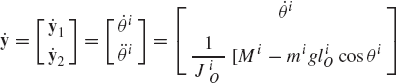
In order to demonstrate the formulation of the state space equations in both cases of the augmented formulation and the formulation in terms of the degrees of freedom, we consider the simple system discussed in Example 10. If the dynamic relationships are formulated in terms of the degrees of freedom using the embedding technique, the system has one differential equation, which can be expressed in terms of this degree of freedom. If we select the angular orientation θi to be the degree of freedom, the differential equation of motion of the system is given by
where JiO = Ji + mi(liO)2 is the mass moment of inertia defined with respect to point O, Ji is the mass moment of inertia defined with respect to the center of mass, mi is the total mass of the rod, mi is the applied external moment acting on the rod, and liO is the distance of point O from the center of mass of the rod. In this example, the vector qi reduces to a scalar defined by the angle θi. The preceding equation then yields
From which the vector Gi of Eq. 165 reduces to a scalar and is recognized as
The state vector is
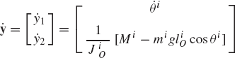
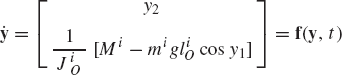
and the state equations can be defined using Eqs. 169 and 170 as
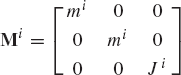
Let us now consider the second approach of the augmented formulation in which the equations are developed in terms of the absolute coordinates Rix, Riy, and θi. In this case, the mass matrix Mi is
The algebraic constraints of the revolute joint are
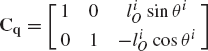
and the constraint Jacobian matrix is
The vector Ct of Eq. 136 is the null vector while the vector qd of Eq. 137 is
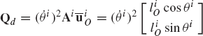
Equation 138 can be constructed for this system as
One can verify that the solution of this system of algebraic equations defines
which is the same equation obtained previously using the degree of freedom of the system as the generalized coordinate. Therefore, the state space equations are the same as obtained previously in this example.
Many of the existing accurate numerical integration algorithms are developed for the solution of first-order differential equations. By putting the dynamic equations in the state space form, one can use many of the existing well-developed numerical integration methods to obtain the state of the multibody system over a specified period of simulation time. In this section, some of these numerical integration methods are discussed, and we shall start with a simple but a less accurate method called Euler's method.
Perhaps the simplest known numerical integration method is Euler's method. While this method is not accurate enough for practical applications, it can be used to demonstrate many of the features that are common in most numerical integration methods. The form of the state space equations given by Eq. 169 can be used to derive Euler's formula for the numerical integration. For this purpose, Eq. 169 is rewritten as
or dy = f(y, t)dt which upon integration leads to
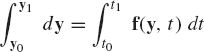
where
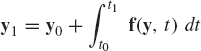
in which t1 = t0 + h, where h is a selected time step, and y0 is the state vector that contains the initial conditions. Equation 172 can be written as
If the time step h is selected to be very small, the integral on the right-hand side of Eq. 174 can be approximated as
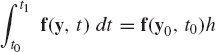
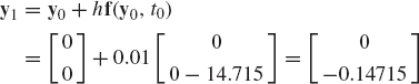
Substituting this equation into Eq. 174, one obtains
By using a similar procedure, one can also show that y2 = y1 + hf(y1, t1). This procedure leads to Euler's method defined in its general form by the equation
where yn = y(t = tn). Equation 177 implies that if the state vector of the system is known at time tn and the step size h is assumed, the right-hand side of Eq. 177 can be evaluated and used to predict the state of the system at time tn+1. Once yn+1 is determined, the procedure can be repeated to advance the numerical integration and evaluate the state of the system at time tn+2. This procedure continues until the end of the simulation time is reached.
As pointed out earlier, Euler's method is not an accurate technique for the numerical integration because of its low order of integration. In order to demonstrate this fact, we write Taylor's expansion for the state vector y at time tn+1 as
where
By dropping terms of an order higher than the first order in h, Euler's method can be obtained from Taylor's series. In this case, the error in the numerical integration is defined by the equation
Being a first-order method (straight-line approximation), Euler's method becomes inaccurate when the state vector is a rapidly varying function of time.
Example 6.12
In order to demonstrate the use of Euler's method for the numerical integration, we consider the simple system of Example 11. We assume that the mass of the body is 1 kg, the distance from the center of mass to point O is 0.5 m and its mass moment of inertia about point O is 0.3333kg · m2. The joint torque mi is assumed to be harmonic function that takes the form
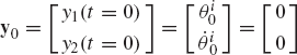
The initial conditions are assumed to be zeros, that is
The state space equations of this system were obtained in Example 11 as
Keeping in mind that y1 = θi and
If JiO = 0.3333kg · m2, mi = 1kg, g = 9.81m/s2, and liO = 0.5m, one has
subject to the initial conditions
If we select the time step for the numerical integration to be h = 0.01s, the solution at time t1 = t0+h = 0.01s is
The solution at t2 = t1 + h = 0.02s can be obtained as

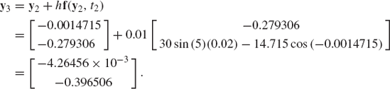
Similarly, the solution at t3 = t2 + h = 0.03s is
This process continues until the desired end of the simulation time is reached.
Euler's method is a single-step method with an order of integration equal to 1. The error resulting from the use of this method is large, especially in the analysis of nonlinear systems. For rapidly varying functions, the use of low-order integration methods is not generally recommended since the error is a function of the frequency content and as the frequency increases the error also increases when these integration methods are used. In order to demonstrate this, we consider the simplest oscillatory system that consists of mass m, which is supported by a linear spring that has a stiffness coefficient k. The equation of motion that describes the free vibration of this system is given by
where x is the displacement of the mass. The exact solution of the preceding differential equation is
where
If we use the exact solution to substitute for x and
and
In Euler's method, first-order approximation is made. Second- and higher-order terms are neglected and the error is in the form defined by Eq. 180. It is clear from this error equation that the first term that appears in the error series is function of
As differentiation continues, the resulting terms become functions of higher power of the frequency ω and, therefore, as the frequency increases, the error resulting from the use of Euler's method increases. For that reason, very low-order numerical integration methods are hardly used in the analysis of nonlinear multibody systems. More accurate numerical integration methods such as the single-step Runge-Kutta methods and multistep Adams-Bashforth and Adams-Moulton methods are often used. While in single-step methods only knowledge of the numerical solution yn is required in order to compute the next value yn+1, in multistep methods several previous values are required.
Runge-Kutta methods are widely used in the numerical solutions of the nonlinear differential equations of mechanical systems. While the order of integration of Runge-Kutta methods is normally higher than one, only knowledge of the function f(y, t) is required since the use of Runge-Kutta methods does not require determining the derivatives of the function f(y, t). One of the most widely used Runge-Kutta formulas is
where
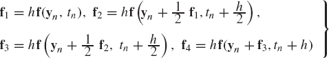
where h is the time step size, and yn and yn+1 are, respectively, the solutions at time tn and tn+1.
In order to demonstrate the use of Runge-Kutta methods, we consider the problem discussed in Example 11. For this example, the vector function f is
and y0 = 0. In order to advance the numerical integration using Runge-Kutta methods, we must evaluate the functions f1, f2, f3, and f4. If h = 0.01s, one has
Using f1, one evaluates
It follows that
The function f2 can be used to evaluate

Therefore, f3 can be evaluated as
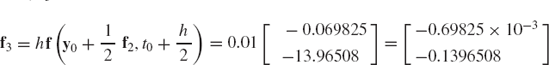
This vector can be used to evaluate y0+f3 as

and
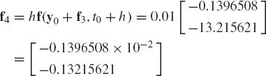
The solution at time t1 = t0+h = 0.01s can be obtained using the Runge-Kutta method as
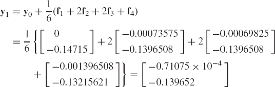
The vector y1 can then be used to predict the solution at time t2 = t1+h. This process continues until the desired end of the simulation time is reached. Clearly, the use of the Runge-Kutta method requires many more calculations as compared to Euler's method, a price that must be paid for higher accuracy.
In the case of a single function y, the general form of the multistep methods is given by (Atkinson, 1978)
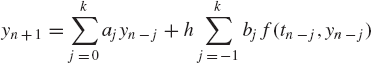
where h is the time step size, tn = t0+nh, a0, ..., ak, b−1, b0, ..., and bk are constants, and k ≥ 0. The multistep method is called the k + 1 step method if k + 1 previous solution values are used to evaluate yn+1. In this case, either ak ≠ 0 or bk ≠ 0. Note that Euler's method is an example of a one-step method with k = 0 and
If the term yn+1 appears only on the left-hand side of Eq. 189, the method is said to be an explicit method. This is the case in which b−1 = 0. If b−1 ≠ 0, yn+1 appears on both sides of Eq. 189 which, in this case, defines an implicit method. In general, iterative procedures are used to solve implicit methods.
An example of an explicit method is the two-step midpoint method defined by the formula
An example of an implicit method is the one-step trapezoidal method defined by the formula
The convergence of the approximate solution obtained by using multistep methods can be proved by defining an error function and requiring that this error function approaches zero as the step size approaches zero. This condition, which is called the consistency condition, can be used to obtain a set of algebraic equations that relate the constants aj and bj of Eq. 189. In general, there are two approaches for deriving higher order multistep methods. These are the method of undetermined coefficients and the method of numerical integration. In the method of undetermined coefficients, the algebraic equations obtained using the consistency condition are used to define the constants aj and bj, while in the method of numerical integration, polynomial approximations are employed. The methods based on the numerical integration are more popular and are used to derive the most widely used multistep methods such as the predictor-corrector Adams methods, where an explicit formula is used to predict the solution at tn+1 using the previous solution values. The predicted solution is then substituted into the implicit corrector formula to determine the corrected solution. Such a solution procedure can be used to control the size of the truncation error.
Adams methods are widely used in solving first-order ordinary differential equations. They are used to obtain predictor-corrector algorithms where the error is controlled by varying the step size and the order of the method. Adams methods can be derived using the method of numerical integration starting with the following equation:
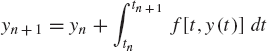
Interpolation polynomials are used to approximate f[t, y(t)], and by integrating these polynomials over the interval [tn, tn+1], one obtains an approximation to yn+1. Two formulas are often used; these are the predictor explicit Adams-Bashforth methods and the corrector implicit Adams-Moulton methods.
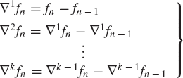
In the explicit or predictor Adams-Bashforth methods, interpolation polynomials Pk(t) of a degree less than or equal to k are used to approximate f(y, t) at tn−k,...,tn. A convenient way of constructing the interpolation polynomials is to use the Newton backward difference formula expanded at tn,
where fn = f(yn, tn) and the backward differences are defined as
The integral of Pk(t) is given by (Atkinson, 1978)
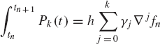
where the coefficients γj are obtained using the formula
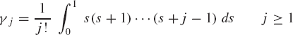
in which s = (t−tn)/h with γ0 = 1. It can also be shown that γ1 = 1/2, γ2 = 5/12, γ3 = 3/8, γ4 = 251/720, and γ5 = 95/288.
The derivation of the corrector implicit Adams-Moulton method is exactly the same as the Adams-Bashforth method except we interpolate f(y, t) at the k+1 points tn+1,...,tn−k+1. The formula for the implicit Adams-Moulton method is

where
with δ0 = 1. It can also be shown that δ1 = −1/2, δ2 = −1/12, δ3 = −1/24, δ4 = −19/720, and δ5 = −3/160. Note that the trapezoidal method is a special case of the Adams-Moulton formula with k = 1. Since the Adams-Moulton formula is an implicit method, the iterative procedure for solving it requires the use of a predictor formula such as the explicit Adams-Bashforth formula. One of the main reasons for using the implicit Adams-Moulton formulas is the fact that they have a much smaller truncation error as compared to the Adams-Bashforth formulas when comparable order is used. Computationally, it is desirable to make the order of the predictor formula less than the order of the corrector formula by one. Such a choice has the advantage that the predictor and corrector would both use derivative values at the same nodes. The second-order Adams-Moulton formula that uses the first-order Adams-Bashforth formula as a predictor is the same as the trapezoidal method that uses the Euler formula as a predictor.
Most of the predictor-corrector algorithms that are based on Adams method control the truncation error by varying both the order and the step size. By using a variable order, there is no difficulty in starting the numerical integration and obtain starting values for the higher order formulas. For instance, the numerical integration begins with the second-order trapezoidal method that uses Euler formula as a predictor, and as more starting values become available, the order of the method can be increased.
The formulation of the dynamic equations using the independent variables leads to the smallest system of strongly coupled equations. The numerical solution of this system that requires only the numerical integration of differential equations defines the independent velocities and coordinates which can be used to determine the dependent coordinates and velocities in a straightforward manner using the kinematic equations. In the augmented formulation, on the other hand, the kinematic constraint equations are adjoined to the system differential equations using the vector of Lagrange multipliers. This approach leads to a large system of loosely coupled equations that can be solved for the accelerations and Lagrange multipliers. The vector of Lagrange multipliers can be used to determine the generalized reaction forces while the independent accelerations are identified and integrated forward in time in order to determine the independent velocities and coordinates. In this approach, the solution for the dependent coordinates requires the solution of the algebraic system of nonlinear constraint equations:
where C is the vector of kinematic constraint equations, q is the total vector of system coordinates, and t is time. A Newton-Raphson algorithm can be used in order to solve Eq. 200 for the dependent coordinates. In this iterative Newton-Raphson algorithm, the independent coordinates are kept fixed to their values that are obtained from the numerical integration. That is, the Newton differences Δqi associated with these independent coordinates are assumed to be zero. The dependent coordinates, on the other hand, are determined by solving the nonlinear algebraic constraint equations using the iterative Newton-Raphson procedure. In the sparse matrix implementation, one can use the following system of algebraic equations in the Newton iterations:
In this equation, Cq is the constraint Jacobian matrix, δq is the vector of the Newton differences of all coordinates, and Id is a Boolean matrix that has zeros and ones only; with the ones in the locations that correspond to the independent coordinates in order to ensure that δqi = 0. The square coefficient matrix in Eq. 201 is sparse, and therefore, sparse matrix techniques can be used to efficiently solve the preceding system of equations. In this sparse matrix implementation, one does not need to identify the sub-Jacobians Cqi and Cqd associated respectively, with the independent and dependent coordinates. Furthermore, there is no need to find the inverse of the matrix Cqd associated with the dependent coordinates. Note also that, for a given constrained system, the locations of the nonzero elements of the sparse coefficient matrix in Eq. 201 remain the same throughout the simulation.
Once the dependent coordinates are determined, the dependent velocities can be determined using the first equation in Eq. 136, which can be written according to the partitioning of the coordinates as dependent and independent as
where the vector Ct, which is the partial derivative of the constraint equations with respect to time, has dimension equal to the number of the kinematic constraints.
As pointed out in the preceding sections, if the kinematic constraints are linearly independent, the independent coordinates can be selected in such a manner that the matrix Cqd is a nonsingular matrix. Since the independent velocities are assumed to be known as a result of the numerical integration of the independent state equations, Eq. 202 can be considered as a linear system of algebraic equations in the dependent velocities. This equation can be used to define the dependent velocities as
An alternative, yet equivalent approach for solving for the dependent velocities is to solve the following linear sparse system of algebraic equations in the total vector of system velocities:

where Id is the same matrix used in Eq. 201. The right-hand side of Eq. 204 is assumed to be known since
Once the generalized coordinates and velocities are determined, the equations for the accelerations and Lagrange multipliers can be constructed as
where all the matrices and vectors that appear in this equation are as defined in Section 7. Equation 205 can be solved for the accelerations and Lagrange multipliers and the independent accelerations can be identified and used to define the independent state equations, which can be integrated forward in time to determine the independent coordinates and velocities.
The main steps for a numerical algorithm that can be used to solve the mixed system of differential and algebraic equations that appear in the analysis of multibody systems can then be summarized as follows:
An estimate of the initial conditions that define the initial configuration of the multibody system is made. The initial conditions that represent the initial coordinates and velocities must be a good approximation of the exact initial configuration.
Using the initial coordinates, the constraint Jacobian matrix can be constructed, and based on the numerical structure of this matrix an LU factorization algorithm can be used to identify a set of independent coordinates.
Using the values of the independent coordinates, the constraint equations can be considered as a nonlinear system of algebraic equations in the dependent coordinates. This system can be solved iteratively using Eq. 201 and a Newton-Raphson algorithm.
Using the total vector of system coordinates, which is assumed to be known from the previous step, one can construct Eq. 202 or equivalently, Eq. 204, which represents a linear system of algebraic equations in the velocities. The solution of this system of equations defines the dependent velocities.
Having determined the coordinates and velocities, Eq. 205 can be constructed and solved for the accelerations and Lagrange multipliers. The vector of Lagrange multipliers can be used to determine the generalized reaction forces.
The independent accelerations can be identified and used to define the state space equations which can be integrated forward in time using a direct numerical integration method. The numerical solution of the state equations defines the independent coordinates and velocities, which can be used to determine the dependent coordinates and velocities as discussed in steps 3 and 4.
This process continues until the desired end of the simulation time is reached.
The selection of the set of independent coordinates is an important step in the computer solution of the constrained dynamic equations. This selection has a significant effect on the stability of the solution and also on reducing the accumulation of the numerical error when the algebraic kinematic constraint equations are solved for the dependent variables. In Section 5, a numerical procedure that utilizes the Gaussian elimination for identifying the set of independent coordinates was discussed. It is necessary, however, in many applications, to change the set of independent coordinates during the numerical integration of the equations of motion.
In order to demonstrate some of the difficulties encountered when the independent coordinates are not properly selected, we consider the closed kinematic chain shown in Fig. 9. Such a closed kinematic chain that consists of nb links connected by revolute joints has nb degrees of freedom. In order to define the chain configuration in the global coordinate system, at least two translational Cartesian coordinates must be selected as degrees of freedom, as shown in Fig. 9. The other remaining degrees of freedom can be selected as rotation angles, and hence there are two rotational coordinates for two links that must be treated as dependent coordinates. The dependent rotational coordinates can be expressed in terms of the independent angles using the loop-closure equations.
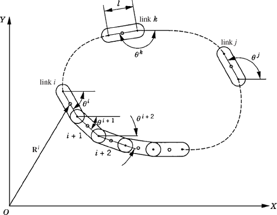
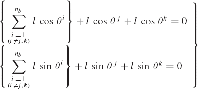
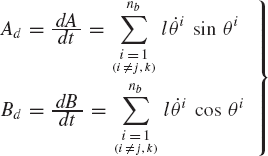
where nb is the total number of the links, θj and θk are the dependent rotation angles of the links j and k, and l is the length of the link. For simplicity, we assumed here that all the links are of equal length. The preceding two equations can be written as
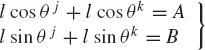
where

By differentiating the resulting loop-closure equations with respect to time, one obtains

These two equations can be rewritten as
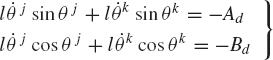
where
It follows that

This system of equations can be solved for
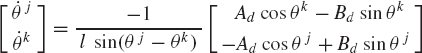
It is clear from this equation that singularities will be encountered when θj −θk is close to or equal to 0 or π. In these situations, an alternate set of independent coordinates must be used; otherwise, a small error in the independent variables will lead to a very large error in the dependent variables.
It is clear from the closed-chain example that if the set of independent coordinates is defined only once at the beginning of the simulation, numerical difficulties may be encountered when the system configuration changes. If the error in the dependent coordinates becomes large, the number of the Newton-Raphson iterations required to solve the nonlinear kinematic constraint equations will significantly increase. Furthermore, the numerical errors in the dependent coordinates may lead to significant changes in the forces and system inertia, which, in turn, make the dynamic equations appear as being stiff, thereby forcing the numerical integration method to select a smaller step size. For this reason, it is recommended that one redefines the set of independent coordinates every few time steps in order to avoid such numerical difficulties. An example of these difficulties was observed in the analysis of the tracked vehicle shown in Fig. 10. A planar model that consists of 54 rigid bodies was used in a numerical investigation (Nakanishi and Shabana, 1994). These bodies, as shown in Fig. 11, are the ground denoted as body 1, the chassis denoted as body 2, the sprocket denoted as body 3, the idler denoted as body 4, the seven lower rollers denoted as bodies 5–11, the upper roller denoted as body 12, and 42 track links denoted as bodies 13–54.

In the model shown in Fig. 11, the idler, sprocket, upper roller, and lower rollers are connected to the chassis using revolute joints. The track is modeled as a closed kinematic chain in which the track segments are connected by revolute joints. The equations of motion of the multibody tracked vehicle was obtained using the augmented approach where the kinematic constraints are adjoined to the dynamic equations using the technique of Lagrange multipliers. Contact force models which describe the interaction between the sprocket, the idler, the rollers, and the track segments were developed and were introduced to the dynamic formulation as a set of nonlinear generalized forces that depend on the system coordinates and velocities. Friction forces between the track segments and the ground were also considered (Nakanishi and Shabana, 1994). In the Lagrangian formulation, the dynamics of the vehicle is described using 162 absolute coordinates and 52 revolute joints that introduce 104 kinematic constraint equations in addition to three ground constraint equations. Because of the joint constraints, the vehicle has only 55 degrees of freedom. The vehicle, however, was driven by rotating the sprocket with a constant angular velocity, and the driving constraint of the sprocket when applied reduces the number of degrees of freedom by one. For the tracked vehicle model shown in Fig. 11, the coefficient matrix of Eq. 205 is a 270 × 270 symmetric matrix.
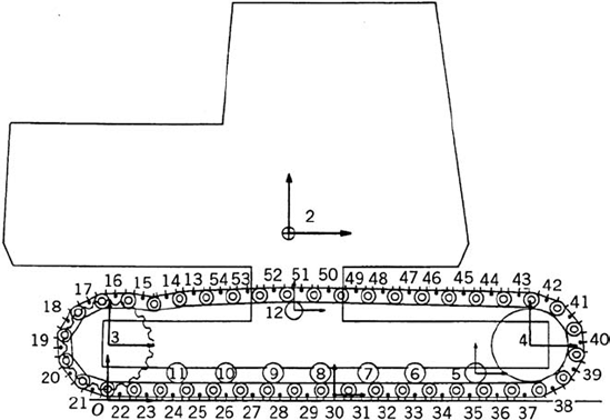
The numerical solution of the tracked vehicle equations was obtained first by using one set of independent coordinates throughout the dynamic simulation. Figure 12 shows the contact forces acting on some of the rollers, while Fig. 13 shows the acceleration of the chassis of the vehicle. From the results presented in these two figures, some unexpected dynamic behaviors can be observed. There was no reason to justify the sudden change in the contact forces and the accelerations shown in Figs. 12 and 13 after 4 s. The sudden increase in the contact forces was found to be the result of the motion of body 24, whose coordinates were all selected as dependent coordinates.
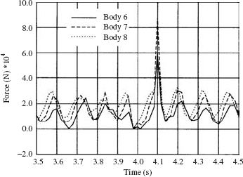
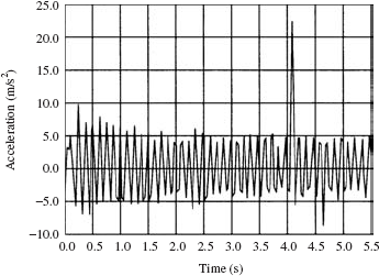
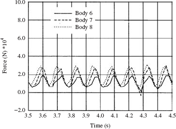

In order to avoid the singular configuration, the dynamic simulation was carried out using different sets of independent coordinates. Before the time of the singular configuration was reached, the set of independent coordinates was changed to include the rotation of body 24. Significant improvements in the results were achieved as the result of changing the set of degrees of freedom. Figures 14 and 15 show, respectively, the contact forces acting on some of the rollers, and the acceleration of the center of the mass of the chassis when different sets of degrees of freedom were used to avoid the singular configurations. Figure 16 shows the results of a computer animation of the vehicle model.
The success of the numerical algorithm based on the coordinate partitioning method, which has been extensively used in multibody system dynamics literature, depends on the convergence of the iterative Newton-Raphson algorithm. A simple approach that can eliminate the need for using the Newton-Raphson method is Baumgarte's constraint stabilization method. Recall that the second time derivative of the constraints can be written as
It is known, however, that the solution of the preceding equation can be an exponential growth, which is the case of an unstable solution. In Baumgarte's method, the equation above is modified and is written in the following form:
where α > 0 and β ≠ 0. The preceding two equations lead to
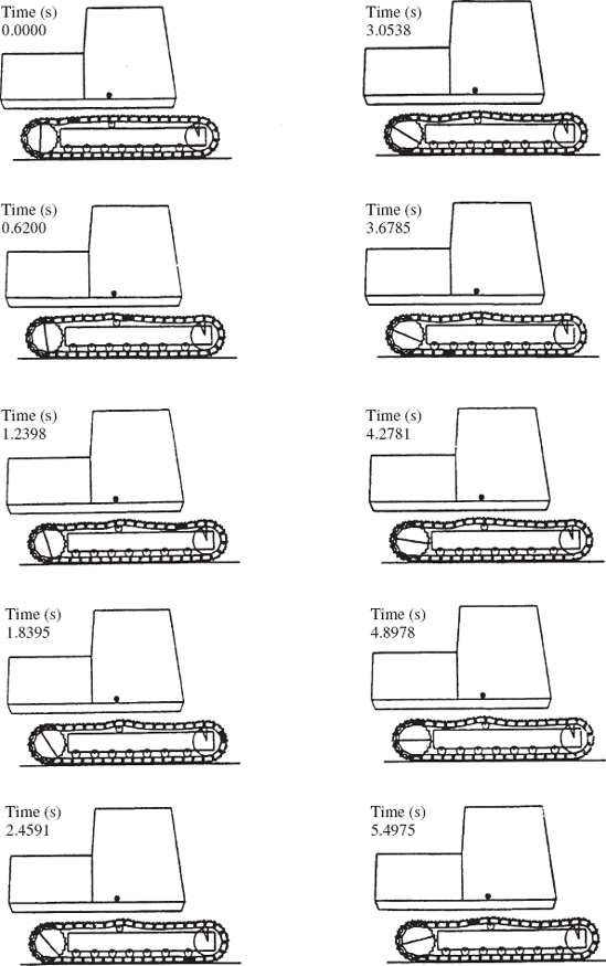
The equations of motion of the system (Eq. 205) can be modified and written as
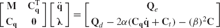
With this modification in the equations of motion, all the accelerations are numerically integrated without partitioning the coordinates into dependent and independent, thereby eliminating the need for the use of the iterative Newton-Raphson method.
While Baumgarte's constraint stabilization method gives accurate results in some applications, there is no known reliable method for selecting the coefficients α and β. Improper selection of these coefficients can lead to erroneous results.
We discussed in Chapter 3 the case of kinematically driven systems in which the number of constraint equations is equal to the number of system-generalized coordinates. In this case, the Jacobian matrix is a square matrix, and if the constraint equations are linearly independent, the Jacobian matrix has a full row rank, and all the system coordinates can be considered as dependent. Equation 200 can then be solved for the system coordinates using a Newton-Raphson algorithm. Once the coordinates are determined, the first equation in Eq. 136 can be considered as a linear system of algebraic equations which can be solved for the total vector of system velocities. The accelerations, however, can be obtained by either using Eq. 136 as discussed in Chapter 3 or by using Eq. 205. In many multibody computer programs, Eq. 205 is used since its solution determines the vector of Lagrange multipliers, which can be used to evaluate the generalized constraint forces, including the generalized driving constraint forces.
The inverse dynamics is the problem of determining the driving joint forces that produce the desired motion trajectories. The procedure for solving the inverse dynamics problem is to define a kinematically driven system by introducing a set of driving constraints that define the prescribed motion. Hence, the position coordinates, velocities, and accelerations of the bodies that form the system can be determined using a standard kinematic analysis procedure as discussed in Chapter 3. Knowing the coordinates, velocities, and accelerations, the equations of motion of the system can be solved as a set of algebraic equations to determine the joint reaction forces as well as the driving constraint forces that are required to generate the prescribed motion. The obtained driving joint forces are often referred to as the feed forward control law. It is expected that when these forces are used to drive the system, the desired motion trajectories will be obtained.
The algorithms for the kinematic and dynamic analyses presented in Chapter 3 and in this chapter can be used to solve the inverse dynamics problem. In order to demonstrate the procedure for solving the inverse dynamics problem using the augmented formulation, we consider the slider crank mechanism shown in Fig. 17. One may be interested in determining the crankshaft torque that produces a specified desired motion of the slider block of the mechanism. Let us assume that the prescribed motion of the slider block is
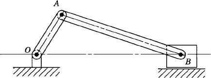
where f(t) is a given function of time. The objective then is to determine the crankshaft driving torque that produces the desired motion defined by the preceding equation. Since the slider crank mechanism has one degree of freedom, the use of the driving constraint defined by the preceding equation leads to the kinematically driven system discussed in Chapter 3. The coordinates and velocities of the bodies in the mechanism can be determined using a kinematic analysis procedure similar to the one discussed in Chapter 3. Once the coordinates and velocities are determined, the vectors of accelerations and Lagrange multipliers can be determined at every time step using Eq. 205. The solution of this equation defines Lagrange multipliers associated with the joint and driving constraints. Lagrange multipliers associated with the driving constraints can be identified and used to evaluate the driving constraint force.
For the slider crank mechanism example, the driving constraint can be written in the following form:
It is clear from this equation that the only nonzero component of the driving constraint force is the component associated with the motion of the slider block. This force component is defined as
where λd is the Lagrange multiplier associated with the driving constraint Cd. The virtual work of the driving constraint force is
In order to determine the crankshaft torque that is required to generate the desired motion of the slider block, we write δR4x in terms of the virtual change in the crankshaft angle θ;2. The loop equations of the mechanism are
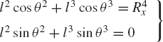
where l2 and l3 are, respectively, the lengths of the crankshaft and the connecting rod, and θ3 is the angle that defines the orientation of the connecting rod. Using the loop equations, one has
Using this equation, the virtual work of the driving constraint force can be written as
or
where M2 is the crankshaft driving torque that is required to generate the desired motion of the slider block. This torque, which defines the feedforward control law, is given by
The simple one-degree-of-freedom slider crank mechanism example discussed in this section demonstrates the use of the augmented formulation and general-purpose multibody computer programs to solve the inverse dynamics problem. A similar procedure can be used in the case of multidegree of freedom systems. For such a multidegree of freedom system, one obtains the driving generalized joint forces associated with the independent joint coordinates.
Another case that can be considered as a special case of the general computational algorithm discussed earlier in this chapter is the case of the static analysis of constrained multibody systems. It is desirable in many applications to obtain the static equilibrium configuration prior to the dynamic simulation. Since in the case of static equilibrium, the velocities and accelerations are assumed to be equal to zero, Eq. 205 reduces to
This equation implies that if the multibody system is in static equilibrium, the generalized constraint forces must be equal to the generalized applied forces. Multiplying both sides of Eq. 227 by the vector δq yields
As described in Section 6 of this chapter, the vector δq of the virtual changes of the system-generalized coordinates can be expressed in terms of the virtual changes of the independent coordinates as
Substituting Eq. 229 into Eq. 228 leads to
Using the fact that CqBi = 0, the preceding equation reduces to
Since the components of the vector δqi are assumed to be independent, the preceding equation reduces to
This system, which has a number of equations equal to the number of independent coordinates, can be written as
where Ri = BTiQe. Equation 233 is a nonlinear system of equations in the system coordinates and can be solved using a Newton-Raphson approach.
Keeping in mind that the kinematic constraints can be used to express the dependent coordinates in terms of the independent ones, the numerical procedure for solving Eq. 233 starts by making a guess for the independent coordinates and use the constraint equations to determine the dependent coordinates. Being able to do this, allows us to write Eq. 233 in terms of the independent coordinates only as
This vector equation can be solved for the independent coordinates using an iterative Newton-Raphson algorithm.
Another alternative, yet equivalent, approach for the static analysis of a multibody system is to consider Eq. 227 with the constraint equations
Equations 227 and 235 represent n + nc nonlinear algebraic equations in the n+nc unknowns q and λ. These two vector equations can be solved for the unknowns using a Newton-Raphson algorithm. The main difficulty in using this approach is the need for having an initial estimate of the vector of Lagrange multipliers.
Figure P1 shows a uniform slender rod that has mass 1 kg. At a given configuration, the velocity and acceleration of the center of mass are given by
The angular velocity of the rod at this point in time is 150 rad/s, while the angular acceleration is zero. Determine the generalized inertia forces associated with the absolute coordinates of the center of mass as well as the rotation of the rod.
Repeat problem 1 assuming that the angular acceleration is 450 rad/s2. What is the kinetic energy of the system and what is the mass matrix.
In problem 1 determine the generalized inertia forces associated with the absolute coordinates of point A as well as the rotation of the rod.
In problem 2 determine the generalized inertia forces associated with the absolute coordinates of point A as well as the rotation of the rod.
In problem 1, what will be the mass matrix if the generalized coordinates are selected to be the absolute coordinates of point A and the angular orientation of the rod? Also calculate the generalized centrifugal forces.
The slender rod shown in Fig. P1 has mass m = 1kg, F = 5N, M = 10N · m, and γ = 45°. Determine the matrix equation of motion of this rod assuming that the generalized coordinates are the absolute Cartesian coordinates of the center of mass and the angular orientation of the rod. Using the obtained equations, determine the accelerations of the center of mass and the angular acceleration of the rod.
Repeat problem 6 assuming that the generalized coordinates are the absolute Cartesian coordinates of point A and the angular orientation of the rod.
For the system shown in Fig. P2, let F = 10N, M = 15N · m, θ = 45°, γ = 80°, and assume that the rod is slender with mass m = 1kg, length l = 1m, and its angular velocity at the given configuration is 150 rad/s. If the generalized coordinates are selected to be the absolute coordinates of the center of mass and the angular orientation of the rod, obtain the matrix differential equations of the system in terms of these coordinates and the reaction forces. Express the absolute accelerations of the center of mass in terms of the angle θ. Use these kinematic relationships with the dynamic equations to determine the numerical values of the acceleration and the joint reaction forces.
In the preceding problem formulate the constraint equations of the revolute joint. Define the constraint Jacobian matrix and use the generalized coordinate partitioning to identify the Jacobian matrices associated with the dependent and independent coordinates. Use the coordinate partitioning to reduce the three differential equations obtained in the preceding problem to one that can be solved to determine the angular acceleration of the rod.
For the system shown in Fig. P3, let M2 = M3 = 15N · m, F = 10N, θ2 = 60°, and θ3 = 45°. The angular velocities of the links are assumed to be

Use the generalized coordinate partitioning of the constraint Jacobian matrix to solve the preceding problem.
For the system shown in Fig. P4, let M2 = 10N · m, M3 = 8N · m, M4 = 5N · m, F4 = 5N, γ = 30°, θ2 = 60°,

Use the generalized coordinate partitioning of the constraint Jacobian matrix to solve the preceding problem.
Develop the differential equations of motion of the slider crank mechanism shown in Fig. P5 in terms of the absolute coordinates. Assume that M2 = 10N · m, F4 = 15N, θ2 = 45°, and

Develop the differential equations of motion of the four-bar mechanism shown in Fig. P6 in terms of the absolute coordinates of each link. Assume M2 = M4 = 5N · m, F3 = 10N, θ2 = 60°, and
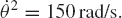
Develop the equations of motion of the system of problem 12 in terms of Lagrange multipliers. Use the computer to solve the resulting system of equations for the accelerations and Lagrange multipliers, and use the obtained solution to determine the generalized and the actual reaction forces.
Develop the equations of motion of the slider crank mechanism of problem 14 in terms of Lagrange multipliers. Solve the resulting system of equations using computer methods in order to determine the accelerations and Lagrange multipliers, and determine the generalized and actual joint reaction forces.
Obtain the differential equations of motion of the four-bar linkage of problem 15 in terms of Lagrange multipliers. Use the computer to solve the resulting system of equations for the accelerations and Lagrange multipliers, and determine the generalized and actual joint reaction forces.
Put the second-order differential equations of motion of the system of problem 6 in the state space form. Using the Runge-Kutta method, develop a computer program for the numerical integration of the state space equations of this system. Plot the angular displacement and velocity versus time for 1 s of simulation time. Use a step size Δt = 0.01s, and assume that the initial conditions are

Develop the state space equations of the system of problem 8. Using the Runge-Kutta method, develop a computer program for the numerical integration of these equations. Plot the angular displacement and velocity of the rod for 1 s of simulation. Assume a step size of 0.005 s and use the configuration described in problem 8 as the initial configuration.
Find the state space equations of the system of problem 10. Develop a computer program based on the Runge-Kutta method for the numerical solution of this system. Plot the solution obtained using this program for 2 s of simulation with a step size Δt = 0.01s. Use the configuration described in problem 10 as the initial configuration.
Obtain the state space equations of the slider crank mechanism of problem 14. Solve these equations numerically using the Runge-Kutta method and plot the position and orientation of the links for one revolution of the crankshaft. Use the configuration described in problem 14 as the initial configuration. Present the solution for two different time step sizes (Δt = 0.001 and 0.005 s) and compare the results.
Obtain the state space equations of the four-bar mechanism of problem 15. Solve these equations numerically using the Runge-Kutta method, and plot the angular displacements and velocities of the links for one revolution of the crankshaft. Use the configuration described in problem 15 as the initial configuration, and use a step size (Δt = 0.001 and 0.005 s). and compare the results.