
Chapter 6
Oscillations and waves
Periodic motion is ubiquitous in nature, from the obvious like heart beats, planetary motion, vibrations of a cello string, and the fluttering of leaves, to the less noticeable such as the vibrations of a gong or shaking of buildings in the wind. Oscillations and periodicity are the unifying features in these problems, including nonlinear systems in Chapter 5. The motion is back and forth repeating itself over and over, and can cause waves in a continuous medium.
We will study periodic motion including oscillations and waves in this chapter. There are two motivating factors for studying these phenomena at this juncture. Physically, waves involve independent motion in both space and time. We can see waves moving along a string (space) and also feel the vibrations in time at a fixed point. We can better understand wave motion after understanding particle motion. Mathematically, waves are described by partial differential equations (PDE) with at least two independent variables such as space and time. We are equipped to tackle PDEs only after studying ODEs first in the previous chapters.
We begin with the discussion of a single, damped harmonic oscillator, and work our way to oscillations of small systems such as triatomic molecules. We then discuss the displacement of a string under static forces. Finally, simulations of waves on a string and on a membrane are discussed.
To solve these problems, we introduce matrix algebra and eigenvalue formulation of linear systems. We also discuss finite difference and finite element methods for boundary value problems involving ordinary and partial differential (wave) equations. Various visualization techniques including animation of waves on strings and membranes using objects in our VPython modules are also presented.
6.1 A damped harmonic oscillator
The best-known oscillator in the physical world is also the simplest: the simple harmonic oscillator (2.46), with its ubiquitous acronym – SHO. Figure 6.1 captures several frames of the animated motion of an SHO over half a period. It is produced with Program 6.1, a slightly modified version of Program 2.1.

Program listing 6.1: Simple harmonic oscillator (sho.py)
import visual as vp
  2
ball = vp.sphere(pos=(−2, −2,0), radius=1, color=vp.color.green) # ball
  4wall = vp.box(pos=(−4, −2,0), length=.2, height=4, width=4)      # wall
floor = vp.box(pos=(0, −3.1,0), length=8, height=0.2, width=4)   # floor
  6spring = vp.helix(pos=wall.pos, thickness=0.1, radius=0.5)        # spring

  8h, v = 0.1, 0.0                                            # step size, initial velocity
while True:
10      vp.rate(50)
      ball.pos.x = ball.pos.x + v*h
12      v = v − ball.pos.x*h                             # Euler−Cromer method
      spring.length = ball.pos.x + 3             # stretch spring (offset by 3)
The spring is drawn as a helix object in VPython (line 6), which has its position at the tail end of the coil (at the wall in this case), and extends in the direction of its axis vector (default to the x-axis, (1,0,0)). The length of the spring is changed as it is being compressed or stretched by the ball (line 13, plus an offset from the wall to the equilibrium position). The integration uses the Euler-Cromer method (line 12), a first-order symplectic integrator for conservative systems (Section 2.4, and Exercise E2.6). The numerical method is stable, and the SHO will oscillate periodically and perpetually according to Eq. (2.47) because there is no dissipation.
Realistic oscillators are dissipative, or damped, due to forces like friction or air resistance. A damped harmonic oscillator of mass m and spring constant k may be described by the linearized version of Eq. (5.30) (small oscillations and a change of variable θ → x) as
![]()
Two generic, system-independent constants are introduced
![]()
where b is the linear coefficient in the damping force, −bv (see Eq. (3.3)).
Given ω0 and the dimensionless γ, Eq. (6.1) is the universal equation for a damped harmonic oscillator. It occurs frequently in physics and engineering problems, and has wide-ranging applications. For example, an RLC circuit (Figure 6.2) behaves exactly like the mechanical oscillator we assumed in Eq. (6.1). The only difference is that the displacement x would be replaced with the charge q (Exercise E6.2).
6.1.1 Critical, over- and under-damping
Let us first examine the solutions of Eq. (6.1) numerically using RK4 for several cases of damping as shown in Figure 6.3.
With no damping, the oscillation is sinusoidal as expected. When damping is small, the oscillation persists but the amplitude is reduced. When damping is further increased to γ ≥ 1, the oscillation is totally wiped out, as the amplitude does not cross the zero axis even once. For the smaller γ = 1, damping happens quicker and more effective than the larger γ = 2. This seems counterintuitive at first, but it is all about the balance of forces. If damping is large, the spring force needs a longer time to restore the system to equilibrium, losing all energy and getting stuck at the equilibrium. The smaller the damping, the faster the process. However, there must be a threshold where if the damping is further reduced, the oscillator will be unable to lose all its energy by the time it returns to equilibrium. If it still has a positive amount of energy left when it reaches the equilibrium position, it will keep going, crossing zero to the other side of the equilibrium. Indeed, this threshold exists (γ = 1, Figure 6.3), and is called critical damping. Below the threshold γ < 1, the oscillation continues, but with reduced peaks and valleys in each cycle, and eventually stops.


Figure 6.3: The damped harmonic oscillator for different damping coefficients γ: no damping, γ = 0; underdamping, γ = 0.2; critical damping, γ = 1; and overdamping, γ = 2.
The numerical results above can be confirmed by analytical analysis [10, 31]. The general solution x(t) to Eq. (6.1) is (Exercise E6.3)
![]()
where A and B are constants, determined by the initial conditions x(0) and ![]() (0). Without damping (γ = 0), Eq. (6.3) reduces to a perfect harmonic (2.47).
(0). Without damping (γ = 0), Eq. (6.3) reduces to a perfect harmonic (2.47).
Because of the overall damping factor exp(−γω0t), the solution will eventually reach zero. We expect this because damping will dissipate all the energy in the system so it stays put at equilibrium. How it gets there, however, is not trivial, and quite interesting as discussed above following Figure 6.3.
Qualitatively, the exponential damping factor is determined by the smaller exponent (A term) in Eq. (6.3), ![]() for γ ≥ 1. Its maximum is 1 when γ = 1, the critical damping – the fastest damping possible. If γ
for γ ≥ 1. Its maximum is 1 when γ = 1, the critical damping – the fastest damping possible. If γ ![]() 1, then
1, then ![]() . The larger the γ, the less effective the damping. This is overdamping.
. The larger the γ, the less effective the damping. This is overdamping.
If γ < 1, the factor ![]() becomes imaginary, so the terms in the brackets of Eq. (6.3) are oscillatory (sinusoidal) functions of time. This leads to underdamping of the kind
becomes imaginary, so the terms in the brackets of Eq. (6.3) are oscillatory (sinusoidal) functions of time. This leads to underdamping of the kind
![]()
where A′ and φ are new constants related to A and B. Both overdamping and underdamping increase the time it takes to reach equilibrium.
6.1.2 Driven oscillator and resonance
In our discussion so far, the system loses energy continuously and stops at equilibrium on its own. What happens if energy is added to the system via an external driving force? We then speak of a driven, linear oscillator. How will it be different from a driven nonlinear oscillator of Section 5.3?
Let the driving force be F(t). We simply add it to Eq. (6.1) to obtain the equation of a driven oscillator
![]()
An interesting case involves a periodic driving force F(t) = Fd cos(ωdt). Given ω0, there are essentially three parameters we can play with: the damping coefficient γ, the driving frequency ωd and amplitude Fd. The amplitude Fd has dimensions of force/mass, but its units are arbitrary depending on the units of x and t.
The results of the driven linear oscillator obtained with RK4 are shown in Figure 6.4 where we vary the driving frequency ωd but keep γ and Fd fixed.
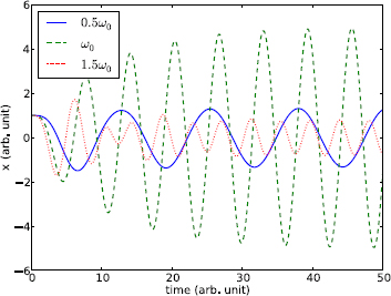
Figure 6.4: The driven harmonic oscillator for different driving frequencies: ωd = 0.5ω0, ω0, and 1.5ω0, with γ = 0.1 and ![]() in each case.
in each case.
The oscillations start out in irregular fashion, but eventually settle into regular sinusoidal oscillations. This happens quicker for critical damping and overdamping, somewhat slower for underdamping. The irregular part of the oscillation is due to transient solutions, and the regular part due to steady state solutions. If we look at the steady state solutions carefully, we find that the oscillation frequency is the same as the driving frequency. This is because damping will cause any initial perturbations to subside, and in the end, the system is responding to the driving force only. Mathematically, the transient solution is the general solution (6.3) to the homogeneous equation (6.1), and the steady state solution is a particular solution to the inhomogeneous equation (6.5) [10].
Unlike the chaotic nonlinear oscillator (Section 5.3), the response of the linear oscillator is proportional to the driving amplitude (see Exercise E6.4). Incidentally, there is no nonlinear dynamics, hence no chaos, in a driven linear oscillator.
Though the driving amplitude is the same in each case, we see a big difference in the steady state amplitudes. For the case shown with relatively small damping, the amplitude is significantly enhanced when the driving frequency is close to the natural frequency, ωd ![]() ω0. This is resonance. The driving force is in near lock-step with the natural oscillation that energy is most easily absorbed, producing an enhanced amplitude.
ω0. This is resonance. The driving force is in near lock-step with the natural oscillation that energy is most easily absorbed, producing an enhanced amplitude.
The general resonance frequency where the amplitude is maximum occurs at (Exercise E6.4)
![]()
Resonance is an important phenomenon in physics and in nature.1 We will see it in quantum transitions (Sections 8.4.2 and S:8.2) and scattering (Sections 12.4.1 and S:8.1.2).
6.2 Vibrations of triatomic molecules
Instead of external driving forces, coupled oscillators can drive each other with internal forces, conserving the energy of the system. Like the simple two- and three-body problems seen before (Section 4.2), Figure 6.5 shows two systems consisting of two and three particles, respectively. We assume the particles are connected by identical springs with spring constant k and unstretched length l. The spring forces could represent bonds in diatomic or triatomic molecules such as CO (C–O) or CO2 (O–C–O), for instance.

Displacement from equilibrium
For the two-particle system, the equations of motion are
![]()
The addition (or subtraction) of l takes into account that, in Hooke's law F = −kx, the variable x refers to the stretching (or compression) of the spring from the unstretched length (l). We can make Eq. (6.7) tidier by measuring the displacement from equilibrium positions. Let ![]() and
and ![]() represent the equilibrium positions of particle 1 and 2, respectively. We then have
represent the equilibrium positions of particle 1 and 2, respectively. We then have ![]() . Introducing new displacement variables as
. Introducing new displacement variables as
![]()
we can rewrite Eq. (6.7) as
![]()
Using the center of mass (CM) coordinates similar to Eq. (4.4),
![]()
we obtain
![]()
The oscillation (u) of two particles is effectively one SHO with angular frequency ω and reduced mass μ. It is a perfect harmonic (2.47).
6.2.1 Numerical solutions and power spectrum
A pair of true coupled oscillators are contained in the three-particle system in Figure 6.5, referred to as the triatomic molecule from now on. We can write down the equations of motion directly in displacement variables ui from Eq. (6.8) as

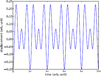
Let us first examine the numerical solutions of Eq. (6.12), which may be solved with a code like Program 6.5. The results are displayed in Figure 6.6. The parameters used are k = 1, m1 = m3 = 1/4, m2 = 2/5, in arbitrary units.2
The initial condition was set to (u1, u2, u3) = (−0.2, 0.2, 0) and zero velocities. Only the displacement u1 is shown (the other two are qualitatively similar). We see regular, periodic oscillations, but they are not sinusoidal. The positive and negative displacements are not symmetric about the equilibrium. The period appears to be 2π for this set of initial conditions.
The nice periodicity in the data tells us that it can be decomposed into a Fourier series to reveal the fundamental frequencies in it. We calculate the power spectrum of the displacement u1 using the FFT method, and show the results in Figure 6.7.
A total of 1,024 data points are used in the Fourier transform. We interpret the spectrum as ranging from negative to positive frequencies, or ωm in [−512, 511] (see Sections 5.5 and S:5.B). There are only five peaks in the spectrum, symmetrically distributed about the origin at ωm = 0, ±10, and ±15. Using the time interval of the data points, we can figure out that they correspond to actual frequencies 0, ±2, and ±3. Since a positive-negative frequency pair ±ω are physically indistinguishable, we conclude that there are three frequencies in the oscillation: ω = 0, 2, and 3. Had we done the same spectrum analysis of the other two particles, we would have found the same frequencies. As we will see next, these are the exact frequencies of the triatomic molecule.

6.2.2 Normal modes
The simulation result in Figure 6.7 shows that the triatomic molecule have discrete frequencies. We can also find these frequencies without numerical integration by a totally different approach: the linear algebraic method. It represents a class of powerful methods involving systems of linear equations and matrix algebra. We introduce this method here, and will rely on it heavily in subsequent problems.
We expect that the solutions to Eq. (6.12) are a superposition of fundamental harmonics (2.47), ui = ai cos(ωt + φ) (see Sec. 3.12 of Ref. [10]). Substituting this form of solution into Eq. (6.12) and rearranging the terms, we obtain

These linear equations may be expressed in matrix form,

Let λ = ω2 and

Equation (6.14) can be more conveniently written as
![]()
The matrix A comes from the coupling forces and is so appropriately named the stiffness matrix because of the spring constants. Note that A is symmetric about the diagonal, i.e., Aij = Aji. The matrix B is due to kinetic energy. For general small oscillations, A and B can be determined systematically from kinetic and potential energies (see Project P6.2).
Equation (6.16) is a so-called (generalized) eigenvalue equation. As we shall see shortly, only discrete, characteristic values of λ are allowed by Eq. (6.16). Moreover, once they are determined, the solutions u can also be found, one for each λ value. A characteristic value of λ is called an eigenvalue, and the corresponding solution u is called an eigenvector, a column vector.
We wish to determine the eigenvalues λ and the eigenvectors u. Linear algebra dictates that (e.g., see Sec. 3.8 of Ref. [10]), aside from the trivial solution u = 0, Eq. (6.16) has nonzero solutions if and only if the determinant is zero

The problem now is to solve for λ from Eq. (6.17), then substitute it back into Eq. (6.16) to obtain u, one for each λ. So an eigenvalue equation like (6.16) determines both the eigenvalues and the eigenvectors.
A direct way to solve Eq. (6.17) is to expand the determinant, which is a cubic polynomial of λ,
![]()
Thus we will have three eigenvalues, or eigenfrequencies. For the parameters used in Figure 6.7, we obtain three eigenfrequencies, ω1 = 0, ω2 = 2, and ω3 = 3 (see Exercise E6.5), in agreement with the Fourier analysis.
Substituting the eigenfrequencies back into Eq. (6.13), we obtain the corresponding unnormalized eigenvectors as

and the final solutions are (up to some phase factors)
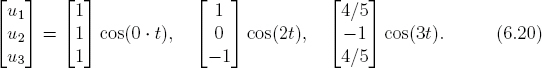
Equations (6.19) and (6.20) are the normal modes. They are the fundamental harmonic oscillations of the triatomic system.
Figure 6.8 shows graphically the motion associated with the normal modes (run Program 6.5 to see animated motion). In mode 1, ω1 = 0, all three particles have the same, constant displacement. There is no oscillation at all. This is the motion of the CM, a pure translation.
In mode 2 (ω2 = 2), the two particles on the sides oscillate about the center particle which stays at rest. The outer particles move in opposite directions of each other with the same amplitude. This is the symmetric stretch. Since the center particle does not participate in the vibration, the frequency is the same as an SHO, namely, ![]() (recall k = 1, m1 = m3 = 1/4 in our example).
(recall k = 1, m1 = m3 = 1/4 in our example).
All three particles vibrate in mode 3 (ω3 = 3), with the outer particles moving in unison, and the center particle vibrating in the opposite direction. This is the asymmetric stretch. The amplitudes of the outer particles are the same, but are smaller than the amplitude of the center particle. Their ratio is such that the CM is at rest in the middle, the same as in mode 2. Any oscillation of the triatomic molecule is a linear superposition of the three normal modes. This is what we have seen in Figure 6.6.

6.2.3 Eigenfrequencies and matrix diagonalization
Direct calculation of eigenfrequencies via determinant expansion as above works for a small system, but quickly becomes unmanageable for larger systems. For an N-particle system, the matrices A, B, and the determinant matrix will have dimensions N × N. There would be N! terms in the determinant alone (merely ~ 3.6 × 10⁶ for N = 10), not to mention a highly oscillatory polynomial. In such cases, matrix diagonalization methods explained below should be used.
To illustrate this, let us assume that in Eq. (6.15) matrix A is already diagonal, and matrix B is the identity matrix.3 Then the determinant in Eq. (6.17) is

Finding eigenvalues of the above equation is simple: they are just the diagonal elements of A.
So, the goal of matrix diagonalization is to nudge a non-diagonal A toward diagonal form while preserving the eigenvalues. It is a complicated business. One of the simpler methods is the Jacobi transformation algorithm for symmetric matrices. It uses a series of rotation transformations to successively eliminate the off-diagonal elements. When the latter are all zero (or close to it), the diagonal elements are the eigenvalues.
Let us illustrate this approach with a very simple example. Suppose N = 2, and B is the identity matrix. Then, matrix A and the eigenvalue equation are
![]()
The Jacobi diagonalization method uses a pair of rotation matrices to transform A to A′ as
![]()
where R(θ) is the rotation matrix (4.75). The rotation R(θ) and its inverse R(−θ) pair are necessary so the transformation is orthogonal and preserves the eigenvalues [10].
Denoting c = cos θ, s = sin θ, and carrying out the matrix multiplication in Eq. (6.23), we arrive at4
![]()
where we have used the symmetry a21 = a12.
We can eliminate the off-diagonal elements by choosing the rotation angle to satisfy
![]()
which yields
![]()
Substituting this θ back into the diagonal elements gives us the eigenvalues.
![]()
which has exact eigenvalues λ1 = 1 and λ2 = 3. According to Eq. (6.25), θ = π/4 which, when substituted into Eq. (6.24), gives the transformed matrix A′
![]()
We see that the diagonal elements are the correct eigenvalues when the off-diagonals are zero.
We can essentially apply the Jacobi transformation to any symmetric N × N matrix, eliminating one pair of off-diagonal elements each time.5 But there is more to it than meets the eye. When N > 2, eliminating one off-diagonal pair introduces nonzero contributions to other off-diagonal elements, though their magnitudes decrease successively [71]. Complications such as stability and convergence must also be addressed when N is moderately large. There are other complicating factors including condition of the matrix, etc. Clearly, the art of solving eigenvalue problems is very involved.
For practical reasons, discussing other algorithms and designing codes that can tackle general eigenvalue problems reliably and efficiently would give us a very limited return within the scope of the text. This is one of the few areas where we defer to “blackbox” solvers for eigenvalue problems. Fortunately, there are several well-tested and widely available open-source packages for such purposes, including BLAS (Basic Linear Algebra Subprograms) and LAPACK (Linear Algebra Package), both available from the Netlib Repository (netlib.org).
We can access BLAS and LAPACK routines in Python via the SciPy libraries (Section 1.3.2), which make available linear algebra functions among other things, at the speed of compiled Fortran codes. For our purpose, the relevant function is eigh(), which solves for eigenvalues and eigenvectors of symmetric (or Hermitian) matrices. The following code solves the eigenvalues of our triatomic molecule. It requires the SciPy library (Section 1.B).
Program listing 6.2: Diagonalization of triatomic systems (eigh.py)
import numpy as np
  2from scipy.linalg import eigh        # Hermitian eigenvalue solver

  4k = 1.0
m1, m2, m3 = 1./4., 2./5., 1./4.
  6A = np.array([[k, −k, 0], [−k, 2*k, −k], [0, −k, k]])
B = np.array([[m1, 0, 0], [0, m2, 0], [0, 0, m3]])
  8
lamb, u = eigh(A, B)       # eigenvalues and eigenvectors
10print (np.sqrt(lamb))      # print omega
The program prepares the matrices A and B according to Eq. (6.15) as NumPy arrays, the expected input format of SciPy routines. The symmetric eigenvalue solver (line 9) takes A and B as input, and returns a pair of arrays: lamb is a 1D array containing the eigenvalues, and u a 2D array filled with the eigenvectors. The i-th column u[:,i] is the eigenvector corresponding to the eigenvalue lamb[i] (see Program 6.6). Executing the program gives the following output:
[ 1.47451053e−08 2.00000000e+00 3.00000000e+00]
We recognize the last two elements are the exact eigenvalues. The first one, however, is not exactly zero. The reason is that ![]() , and λ was “zero”, as far as the computer is concerned, on the order of machine accuracy 10−16 for double precision (Section 1.2).
, and λ was “zero”, as far as the computer is concerned, on the order of machine accuracy 10−16 for double precision (Section 1.2).
For larger matrices, it is more efficient to use sparse matrix functions from SciPy.6 We will encounter this and other linear algebra routines in the sections and chapters ahead.
6.3 Displacement of a string under a load
Suppose we attach an extra atom to the triatomic system of Figure 6.5 and wish to know how this will affect its motion. Well, this does not pose a serious problem. We could follow the same procedure and integrate a four-particle system in place of a three-particle one (6.12). What about five-, six-, or N-particle systems, where N may be very large (think N ~ 1023)? We now have a string of atoms forming a continuous system which can support wave motion. There is no hope of treating this many atoms individually even with all the computing resources in the world combined. Nor would we want to if we want to make sense of collective vibrational and wave motion. Here, we must treat the string as a continuous mass and use concepts such mass density found in continuum mechanics.
6.3.1 The displacement equation
Before studying vibrations on a string, we discuss a simpler problem: the shape of an elastic string in equilibrium under a static, external force. Consider a piece of string between x and x + Δx illustrated in Figure 6.9.

We denote the transverse displacement by u. The piece is held by three forces, the tension to the left T1 = T(x) and to the right T2 = T(x + Δx), and the external transverse load f which is defined as force per unit length. The equilibrium condition is that the longitudinal (horizontal) and transverse (vertical) forces cancel each other, namely,
![]()
![]()
Equation (6.26a) tells us that the longitudinal tension, T = T(x) cos(θ), is the same throughout the string. It is a parameter measuring how stretched (tautness) the string is.
Rewriting Eq. (6.26b) in terms of T gives us
![]()
The net transverse tension force is T tan θ2 − T tan θ1. Since tan θ1 = u′(x), and tan θ2 = u′(x + Δx), we can rearrange Eq. (6.27) to read
![]()
In the limit Δx → 0, the ratio in the first term becomes a second derivative of u, and we have
![]()
This equation describes the displacement of an elastic string under an external load f(x). It is an example of a problem reducing to a differential equation under infinitesimal changes mentioned in Chapter 2.
Given f(x), Eq. (6.29) can be solved if boundary conditions are specified. For instance, if f(x) = f0 is a constant, then
![]()
where a and b are constants to be determined by the boundary conditions u(0) and u(L) at the ends 0 and L, respectively. We see that it is a parabola.
6.3.2 Finite difference method
For a general f(x), we can solve Eq. (6.29) using the finite difference method (FDM). Without loss of generality, we assume the two ends of the string are separated by a distance (L) of unity at x = 0 and x = 1. We divide the distance into N equal intervals, each size h (Figure 6.10). There are N + 1 grid points, including N −1 interior points and two boundary points. Over the grid, let xi = ih, u(xi) = ui, and f(xi) = fi, i = 0, 1, 2, …, N. The boundary points are at u0 and uN.

Once space is discretized, we can approximate the derivatives by numerical differentiation using a three-point central difference scheme. By adding or subtracting the Taylor series such as in Eqs. (2.9) and (2.10), we obtain the first and second derivatives as
![]()
![]()
Equation (6.31a) is the same as the midpoint method (2.13), and the error in both cases is second order in h.
Substituting the discretized second derivative (6.31b) into (6.29) at grid point i, we obtain the FDM displacement equation
![]()
We have simplified the LHS by moving h2 and T to the RHS. We also restrict the grid points to the interior points only. This is a three-term recursion relation, a result of three-point approximation of the second derivative. Even so, all the N − 1 equations must be solved simultaneously since a single grid point can propagate its influence through its neighbors to its neighbors’ neighbors, etc.
Defining gi = −h2fi/T, we can write out Eq. (6.32) explicitly, ending up with

The first and the last rows on the LHS have two terms since we have moved to the RHS the boundary values which are given and need not to be solved. That is how the boundary conditions determine the solutions. The other rows have three terms each.
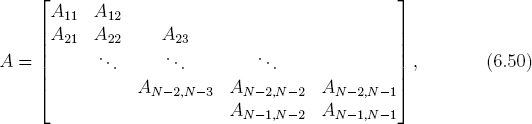
In matrix form, we have a tridiagonal system,

We can express it in compact matrix form
![]()
where A is the (N − 1, N − 1) tridiagonal matrix (stiffness like), B the column matrix on the RHS (N − 1, 1), and u as usual is a column vector containing the N − 1 unknowns u1, u2, … uN−1.
Equation (6.34) (or (6.35)) is a linear system of equations. It can be solved by linear equation solvers once the load f(x) is given, and thus B known. For example, assuming zero boundary values u0 = uN = 0, matrix B for a constant load f(x) = f0 is simply

6.3.3 Solutions of linear system of equations
There are well-known methods for solving a linear system of equations, including Gauss elimination and a closely related variant, the Gauss-Jordan elimination. These methods plus the iterative Gauss-Seidel method are discussed in Appendix S:6.A. Programs implementing these methods are included in Program S:6.1.
However, in keeping with our approach to eigenvalue problems, we will use LAPACK routines via SciPy which provides a general purpose solver solve(A, B). Below we illustrate its use in solving Eq. (6.34).
First let us consider the external force to be constant, f(x) = f0. The program below solves Eq. (6.34) for this case.
Program listing 6.3: String under external forces (stringfdm.py)
  1from scipy.linalg import solve         # SciPy linear eqn solver
import numpy as np, matplotlib.pyplot as plt
  3
N, u0, uN= 20, 0., 0.                 # number of intervals, boundary values
  5x = np.linspace (0., 1., N+1)     # grid
h, T, f = x[1]−x[0], 1.0, −1.0    # bin size, tension, load
  7
A = np.diag([−2.]*(N−1))       # diagonal
  9A += np.diag([1.]*(N−2),1) + np.diag([1.]*(N−2), −1) # off diagonals

11B = np.array([−h*h*f/T]*(N−1))          # B matrix
B[0], B[−1] = B[0]−u0, B[−1]−uN      # boundary values, just in case
13
u = solve(A, B)                                    # solve
15u = np.insert(u, [0, N−1], [u0, uN])      # insert BV at 1st and last pos

17plt.plot(x, u, label=’$f=-1$’), plt. legend(loc=’center’)  # legend
plt.xlabel(’$x$’), plt.ylabel(’$u$’), plt.show()
After setting the number of intervals, the boundary values and related parameters, the program generates matrix A according to Eq. (6.34). First, the diagonal of A is created using np.diag(a,k) (line 8), which returns a 2D array with the k-th (default 0) diagonal given by the 1D input array a. It can also extract the diagonal from a 2D input array (not used here). The next line fills the upper and lower diagonals (k = ±1, and one fewer element than the diagonal), respectively, completing the tridiagonal matrix A. Next, matrix B is created (recall gi = −h2 * f/T, Eq. (6.36)), and the boundary values are accounted for. Once A and B are prepared, solve() from SciPy is called to obtain the solution u (line 14). It contains the displacements at the interior grid points.
Before plotting the results, the two boundary values are inserted into array u, one at the beginning and one at the end. The pair of lists [0,N-1] and [u0,uN] in the np.insert function (line 15) will insert u0 before the first element (index 0) and uN before (the yet nonexistent) index N − 1 which is one position behind the last element, effectively appending to the end (recall that the length of u was N − 1, with the last element at index N − 2). Finally, the results are plotted with legends from the labels given to the curves (line 17).
Figure 6.11 shows the results for two external forces: a constant force f = −1, and a linear force f = −2x (per unit length, of course). The tension parameter is T = 1 in both cases, and the space between the end points were divided into twenty intervals, N = 20. Because the forces are negative, the string droops downward as it is being pulled down by the forces. For the constant force, the shape is a perfect parabola as expected from the analytic solution (6.30), and is symmetric about the center point.

For the linear force, the magnitude of the load increases linearly with x, so the symmetry is broken. The string is sheared toward the right end. The bottom of the valley is shifted to x ~ 0.6, instead of at the center in the case of constant load. The shape can be described by a cubic polynomial. Even though the FDM method is second order, and should be exact only for a second-order polynomial, it turns out that the solutions are actually exact in this case due to a quirk.
The FDM method can be used for any continuous load distribution f(x). If the load is a point source acting on a single point, say a Dirac function f(x) = f0δ(x − x0) (see Section S:5.1, Figure S:5.1), then the point x0 must be treated separately. A different method to be described below, however, can deal with point sources gracefully.
6.4 Point source and finite element method
The finite element method (FEM) is complementary to FDM, but is more versatile and advantageous for certain problems such as point sources just mentioned and irregular domains in higher dimensions. The FEM is commonly used in science and engineering.
Below we introduce FEM in 1D space, which will also be extended to 2D in Chapters 7 and 9. The development of FEM consists of four steps: choosing the elements and basis functions; converting a differential equation to integral form; applying boundary conditions; and finally assembling system matrices and solving the resultant linear system of equations.
6.4.1 Finite elements and basis functions
In FEM, the space is divided into discrete elements. Figure 6.12 shows an example with N = 4 elements labeled e1 to e4. Each element ei has a length hi, which need not be the same. To keep things tidy, we will assume the elements are identical, h1 = h2 = · · · = hN = h. There are N + 1 grid points, called nodes in FEM. The positions of the nodes are xi = ih, same as in FDM.

The difference between FEM and FDM is that, rather than discretizing the differential operator, the FEM tries to interpolate the solution over the domain. To that end, we expand the solution (displacement) u in a basis set as
![]()
where ui are the expansion coefficients to be determined, and φi the basis functions.
In general, the basis functions are arbitrary. For instance, orthogonal basis functions are often used in physics (Sections 9.4 and S:8.2). However, it is crucial to FEM that the basis functions be chosen such that only neighboring basis functions overlap (the reason will be clear in a moment).
The simplest function between two points is a straight line. We construct a basis function φi centered at node i, consisting of two such lines and making a tent-shaped function shown in Figure 6.12. In terms of node number i and width h, we can write it as

The basis function φi is nonzero only in the two elements sharing the common node i. Functions of this type are said to be compact support. Furthermore, φi is unity at node i and zero at other nodes,
![]()
where δij is the Kronecker delta function, δij = 1 if i = j, and 0 if i ≠ j.
Therefore, the solution u (6.37) at node i is
![]()
In other words, the value of the solution at xi is just the expansion coefficient, ui.

Figure 6.13 illustrates the interpolation of the function y = 4x(1 − x) (logistic map) over the unity interval with four finite elements, spanned by five basis functions. Setting ui = y(xi), the values u0 to u4 are ![]() , so the interpolated function is
, so the interpolated function is ![]() . Over each element, the function is approximated by a straight line. It shows that the more elements are used, the more accurate the interpolation.
. Over each element, the function is approximated by a straight line. It shows that the more elements are used, the more accurate the interpolation.
We will need the derivatives of the basis functions later. They are

The derivative is discontinuous at node i. The discontinuity at the nodes is carried over to interpolation (Figure 6.13).
6.4.2 Integral form of solutions
Having chosen the basis functions, we next turn our attention to finding the coefficients ui. Instead of solving Eq. (6.29) directly, FEM solves the integral form (also called the weak form) of the equation [7].
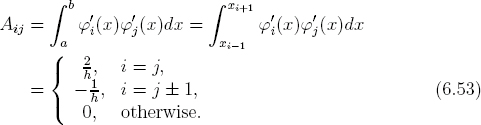
Multiplying both sides of Eq. (6.29) by φj(x) and integrating over the interval [a, b] (which are the end points of the domain) leads to
![]()
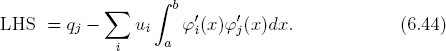
Integrating the LHS by parts, we have
![]()
The quantity qj is zero unless j = 0 or j = N because of the basis function evaluated at the boundaries, i.e., qj = u′(b)δjN − u′(a)δj0.
We differentiate Eq. (6.37) as ![]() , and substitute it into Eq. (6.43), obtaining
, and substitute it into Eq. (6.43), obtaining
Now let
![]()
Because the basis functions and their derivatives have no overlap unless they share a common node, we see that Aij = 0 unless i = j or j ± 1. This is the reason the basis functions are chosen to be compact support, so the matrix Aij is sparse. It is also symmetric, Aij = Aji.
With Eqs. (6.44) and (6.45), Eq. (6.42) can be expressed as
![]()
This is a system of N + 1 linear equations, one for each node. Explicitly, Eq. (6.46) can be expanded as

Equation (6.47) is the final form of the FEM approach. Except for the first and last rows with two terms each, all other rows have three terms, reflecting the fact only neighboring elements contribute to matrix Aij.
6.4.3 Boundary conditions
The unknowns ui in Eq. (6.47) depend on the boundary conditions, q0 and qN. There are two types of boundary conditions.
The Neumann boundary condition specifies the derivatives, u′(a) and u′(b). According to Eqs. (6.39) and (6.43), we replace q0 = −u′(a) and qN = u′(b) in Eq. (6.47). All N+1 node values, u0 to uN, can be determined in the Neumann boundary problem as

The other type is the Dirichlet boundary condition, in which the boundary values u(a) = u0 and u(b) = uN are specified. We are mainly interested in this type of boundary conditions here. Because u0 and uN are already given, we need not to solve for them. We therefore cross off the first and the last rows in Eq. (6.47). Furthermore, we move the first term A10u0 in the second row, and the last term AN−1,NuN in the second to last row, to the RHS. The remaining rows form a linear system of N − 1 equations, which determine the N − 1 interior node values, u1 to uN−1,

In matrix form, let

The solutions in the Dirichlet boundary problems are given by
![]()
In both FDM and FEM, we end up with a linear system like Eq. (6.35) or (6.52). The difference lies in how the boundary conditions are treated, and how the system matrices are set up.
6.4.4 Assembling system matrices
Matrix A in FEM is independent of load. From Eqs. (6.41) and (6.45), we find that the integral over the domain is effectively over the elements ei and ej only,
The full matrix A reads

This is the stiffness matrix in FEM (Dirichlet type), with a dimension (N − 1)×(N −1). It is the same as the FDM stiffness matrix (6.34) (for identical elements of same size h).
For a given load, matrix B will be evaluated according to Eqs. (6.45) and (6.51), where pi given by
![]()
Here we have again used the fact that φi(x) is nonzero only if xi−1 ≤ x < xi+1. For constant load f(x) = f0, pi = hf0. Assuming u0 = uN = 0, matrix B is

Once A and B have been prepared, we can obtain the solutions by solving either Eq. (6.48) for the Neumann boundary type or (6.52) for the Dirichlet boundary type. Comparing the system matrices between FDM and FEM in this case, we find that they are the same (besides the placement of h), so the solutions are identical. It turns out they are also identical for linear load, and differences start to develop only for quadratic and higher order load.
6.4.5 Point source solutions

For a point source, the FEM is easier to apply. For example, consider the following load,
![]()
The Dirac δ function (see Section S:5.1 and Figure S:5.1) makes direct evaluation of f(xn) impossible in FDM. In FEM, however, it poses no special difficulty for this integrable singularity, as
![]()
where we have used the property φn(xn) = 1 from Eq. (6.39). All elements of B are the same as Eq. (6.56) except at node n, where it is (hf0 + α)/T. Solving for u using this modified B, we obtain the results shown in Figure 6.14.
With only a single point-source force, the solution consists of two segments of straight lines. It is what we expect if we pull a string and hold it in position. The “kink” at the point of the applied force indicates a discontinuity of the first derivative, i.e.,7
![]()
If the force is suddenly withdrawn, as if plucking the string, we expect waves to be formed on the string. This is discussed shortly.
When there is an additional constant load, the same discontinuity exists. On each side of xn, the string is a shallower curve relative to the constant force alone, akin to pulling up a suspended cable.
6.5 Waves on a string
When a string, held by a point-like force as depicted in Figure 6.14, is released, wave motion will be generated on it. If the string is coupled to a sound chamber such as that of a cello, vibration energy of the string will be transferred to the chamber, and musical notes can be heard. Modeling the energy loss would be similar to but more complicated than damping in a harmonic oscillator (Section 6.1). We are interested instead in describing an ideal vibrating string without dissipation.
6.5.1 The wave equation
The starting point for the wave equation is Figure 6.9 and Eq. (6.28). The net (transverse) force per unit length on the piece of string from x to x + dx is given by Eq. (6.28),
![]()
where T is the tension, f the external load. For a static string, the net force is zero, giving us the displacement equation (6.29).
For a vibrating string, this is no longer the case. The displacement depends on both position x and time t, u = u(x, t). From Newton's second law, the net force (per unit length) is equal to the linear mass density (ρ) times acceleration. The acceleration at x is given by ∂2u/∂t2, the second derivative of displacement holding x constant. Replacing u″ by ∂2u/∂x2 in Eq. (6.60), we obtain
![]()
The above equation describes the general motion of a string under an external load f.
For a free vibrating string, f = 0, and we have the following wave equation,

Here, v is the speed of the wave. It increases with increasing tension or decreasing mass density.8
So far we have mostly dealt with ODEs. The wave equation (6.62) is a PDE. In general, it is much harder to solve PDEs than ODEs because a PDE has at least two independent variables whereas an ODE only one. We have systematic methods such as the Runge-Kutta scheme that are applicable to most initial value problems involving ODEs. For PDEs, however, few such widely applicable approaches exist. The correct method depends on the kind of problems, and the type of boundary conditions.
6.5.2 Analytical properties
Before solving Eq. (6.62) numerically, we describe analytic properties as a guide to our subsequent discussions. If u(x) is a solution at t = 0, then u(x ± vt) is also a solution. Because Eq. (6.62) is linear, we can form a superposition of counter-propagating waves as
![]()
with A and B being constants. The function f(x−vt) describes a traveling waveform to the right, for if ϕ = x − vt is kept constant, then a fixed value f(ϕ) moves to the right (positive x direction) with speed v. Conversely, g(x + vt) is a traveling wave to the left. Whether f or g (or both) is present depends the initial condition.
A useful technique for PDEs is the separation of variables that can help reduce the dimensionality. Let us try a solution which is a product of space and time variables separately,
![]()
Substitute it into Eq. (6.62) and rearrange the resulting equation so that x and t are on the opposite sides as
![]()
For Eq. (6.65) to hold for all x and t which can vary independently, each side must be a constant, call it −k2,
![]()
The solutions are
![]()
from which we can construct the general solution
![]()
We have four constants (C, k, ϕ, θ) to be determined by the initial condition [u(x, 0), ∂u(x, 0)/∂t], and by the boundary condition [u(0, t), u(L, t)].
Let us consider the case where the two ends of a string are held fixed at zero, u(0, t) = u(L, t) = 0. Equation (6.68) dictates that
![]()
The first term can be satisfied by choosing ϕ = 0. The second term implies
![]()
meaning that only discrete values of wavevector k are allowed.
![]()
The corresponding discrete solution follows from Eq. (6.68),
![]()
This is a standing wave. The λn and fn defined in Eq. (6.71) are the fundamental wavelengths and frequencies (eigenfrequencies). The lowest fundamental frequency is v/2L, and higher harmonics are integer multiples of that. Equation (6.72) is called an eigenmode. The general solution is a linear superposition of all eigenmodes like the normal modes (Section 6.2.2).
6.5.3 FDM formulation
Let us try to numerically solve the wave equation using FDM. We need to discretize both space and time. As before, let the space interval be h, and xm = mh, m = 0, 1, 2, …, N. For time, let Δt be the time interval, and tn = nΔt, n = 0, 1, 2, …. The displacement at xm and tn is written as ![]() , so the subscript refers to space, and the superscript to time.
, so the subscript refers to space, and the superscript to time.
We use the second-order approximation for the derivatives (6.31b),
![]()
![]()
Evaluating the above at xm and tn, and substituting into Eq. (6.62), we have
![]()
The terms on the LHS refer to different space grids at the same time grid, whereas the reverse is true on the RHS.
For stepping forward, we solve for ![]() from Eq. (6.74), obtaining
from Eq. (6.74), obtaining
![]()
This is the FDM form of the wave equation. It is a recursion relating the solution at tn+1 to the solutions at previous two steps tn and tn−1 (for all space grid points). The wave equation is a second-order differential equation, so we expect to have two initial values to determine the solution.
6.5.4 Von Neumann stability analysis
As discussed earlier (Section 1.2.2), recursion relations notoriously tend to be bimodal, either they are very stable or very unstable. If it is unstable, the recursion relation is useless numerically, as a small error will be amplified exponentially, totally overwhelming the true solution. Therefore, before we plunge ahead solving Eq. (6.75) iteratively (or using any recursions), we need to be sure of its stability. We can check this from the von Neumann stability analysis.
Essentially, we represent the solution ![]() as
as
![]()
where ρ and k are constants. The recursion is stable if |ρ| ≤ 1.
To find ρ, we substitute Eq. (6.76) into (6.75). After cancellations and simplification, we obtain
![]()
This is the von Neumann characteristic equation. It has two roots,
![]()
The dividing line is |1−2β2s2| = 1, corresponding to βs = 1, or vΔts = h. If |1−2β2s2| > 1, or vΔts > h, we have two real roots. However, one of them is always greater than unity, so it is unstable.
If |1 − 2β2s2| ≤ 1, or vΔts ≤ h, the two roots are complex conjugates of each other,
![]()
such that the magnitude is unity
![]()
Because s = sin(kh/2) ≤ 1, the sufficient condition for stability is
![]()
Physically, this means that the time step must be smaller than the time it takes for the wave to travel one space grid.
It is instructive to note that if vΔt s is slightly greater than h, then Eq. (6.81) will not be satisfied near the maximum s = sin(kmaxh/2) = 1, i.e., at kmaxh/2 = π/2, or,
![]()
This is just the Nyquist sampling theorem (S:5.44) (Section S:5.B). If we take Δk = 2kmax and Δx = h as the uncertainties in wavevector and in position, respectively, we can restate Eq. (6.82) as ΔpΔx = ħΔkΔx = 2πħ, which satisfies Heisenberg's uncertainty principle. Moreover, using k = 2π/λ, we have from Eq. (6.82)
![]()
which is the minimum wavelength representable over space intervals of h.
6.5.5 Simulation of wave motion
From the above analysis, we can now solve Eq. (6.75) iteratively and maintain stability by choosing β ≤ 1, the single parameter in the wave equation. We use two arrays to hold the solutions at times tn−1 and tn, advance the solution to tn+1 and store it in a third array, then swap the appropriate arrays to advance to tn+2, and so on. This is done in Program 6.4.
Program listing 6.4: Waves on a string (waves.py)
import numpy as np, visual as vp, vpm
  2
def wavemotion(u0, u1):
  4       u2 = 2*(1−b)*u1 − u0                              # unshifted terms
       u2[1:−1] += b*(u1[0:−2] + u1[2:])         # left, right
  6       return u2

  8def gaussian(x):
      return np.exp(−(x−5)**2)
10
L, N = 10.0, 100                # length of string, number of intervals
12b = 1.0                               # beta ˆ2
14x, z = np.linspace (0., L, N+1), np.zeros(N+1)
u0, u1 = gaussian(x), gaussian(x)
16
scene = vp.display(title =’Waves’,background=(.2,.5,1),center=(L/2,0,0))
18string = vpm.line(x, u0, z, (1,1,1), 0.05)            # string

20while(True):
     vp.rate(100), vpm.wait(scene)                     # pause if key press
22     u2 = wavemotion(u0, u1)
     u0, u1 = u1, u2                                             # swap u’s
24     string.move(x, 2*u0, z)                                # redraw string
To start the iterative process, we need the initial solutions at two successive steps. There are several ways to do this. A practical way is to choose u0, then shift it by an amount proportional to vΔt and set it to u1. We use the simplest choice in Program 6.4: we set both to the same Gaussian.
A more important issue is how to handle boundary conditions. When m = 0, for instance, we need ![]() from Eq. (6.75), which is not defined on our grid. The simplest choice is to keep both ends fixed,
from Eq. (6.75), which is not defined on our grid. The simplest choice is to keep both ends fixed, ![]() , so we do not have to worry about them. This is the approach taken in Program 6.4. Or we could use periodic conditions,
, so we do not have to worry about them. This is the approach taken in Program 6.4. Or we could use periodic conditions, ![]() and
and ![]() . It is equivalent to identical strings placed to both the left and right sides of the grid. A string with one end fixed and one end open could also be considered (Project P6.6).
. It is equivalent to identical strings placed to both the left and right sides of the grid. A string with one end fixed and one end open could also be considered (Project P6.6).
Rather than looping through the array index explicitly, wavemotion() iterates Eq. (6.75) implicitly via element-wise operations of NumPy arrays. Whereas the former may seem more direct, the latter is more suitable in terms of speed and simplicity. At a given grid m, the last term in Eq. (6.75) involves the sum of the left and right neighbors, ![]() . It suggests a sum of the form Hj = aIj−1 + bIj + cIj+1 can be done via shifting and slicing, illustrated in Figure 6.15 for a 5-element array.
. It suggests a sum of the form Hj = aIj−1 + bIj + cIj+1 can be done via shifting and slicing, illustrated in Figure 6.15 for a 5-element array.
We can see from the shaded elements that, except for the end points, the interior elements (middle row) are lined up with their neighbors with the shifted arrays. We could accomplish the conceptual shifting via slicing of NumPy arrays (Section 1.D). Guided by Figure 6.15, we can find Hj by
Note that I[1:−1] is the same as I[1:4] for a 5-element array.

Using this strategy, wavemotion() has the uncanny resemblance to the written form of Eq. (6.75), reproducing it almost verbatim: line 4 corresponds to the first two terms in Eq. (6.75), and the next line to the third term via slicing. We gain not only speed, but also simplicity. Because discretized operators like Eq. (6.31b) always involve coupling of close neighbors, we will often encounter such situations. As a result, element-wise operations with slicing will be the preferred method from now on.
The main program animates waves on a string with both ends fixed. The pair of statements (lines 18 and 24) work together to create and redraw the string using the VPM (VPython modules, Program S:6.4) library functions line() and line.move(), respectively. The animation can be paused by a key press (line 21).
Figure 6.16 displays the results from Program 6.4. It shows a single Gaussian peak in the beginning. As time increases, it splits into two smaller peaks, traveling in opposite directions. When they reach the boundaries, there is no possibility of moving forward. The tension is downward, pulling the string in that direction. As a result, the displacement is inverted, and the waves move toward each other, until they merge into one. Thereafter, they split again, repeating the cycle.
The fact that there are two counter-propagating waves is a result of our choice of initial conditions and the principle of linear superposition (6.63). By choosing the two initial waves to be the same, we are in effect forcing two waves into one. It shows we can choose the kind of wave by setting the appropriate initial conditions, from traveling waves to standing waves.
We have used a combination of h and Δt such that β = 1 in Program 6.4. From the von Neumann stability analysis (6.81), this is the maximum β for stable solutions. Could we obtain more accurate solutions if we had used a smaller Δt? Our experience and expectation would tell us yes. As it turns out, we would be wrong in this case: we would get worse, less accurate solutions. Owing to a quirk in the 1D wave equation (6.62), we actually obtain the exact solution if β = 1. The quirk has to do with the fact ∂4u/∂x4 = v−4∂4u/∂t4 [24]. By a happy accident, this leads to total cancellation of the third and higher order terms in the discretized wave equation (6.62) if β = 1. For 1D waves, the optimal value is β = 1, which simplifies Eq. (6.75) to

![]()
This result is almost too simple to be true.
However, the exact algorithm is striking in the symmetry about space and time. Re-writing Eq. (6.84) as
![]()
it tells us that the sum of the amplitudes at a grid point m immediately before and after the current time is equal to the sum of the amplitudes at the current time n immediately ahead and behind the current grid point.
6.6 Standing waves
Like the normal modes for a systems of particles, standing waves are the fundamental building blocks of waves on a string. Any wave can be represented as a linear superposition of these fundamental harmonics (6.72).
Standing waves can be formed by proper choice of initial conditions and their time-dependent motion can be simulated with Program 6.4. Even though analytically solvable (Eq. (6.71)), we are interested in computing the fundamental frequencies using the same FDM scheme as the simulations.
The standing waves satisfy Eq. (6.66)
![]()
subject to the boundary condition X(0) = X(L) = 0. Equation (6.86) is analogous to the static string equation (6.29) if T = 1 and f(x) = k2X. Thus, we can solve it by following the same steps as in Section 6.3.2. In particular, the FDM equation (6.34) as applied to Eq. (6.86) becomes

This is an eigenvalue problem, AX = λX, analogous to Eq. (6.16) but simpler since ![]() . It can be solved using the same method as in Program 6.2 with the eigenvalue solver eigh(). This is done in Program 6.6. The results for the first few standing waves are shown in Figure 6.17.
. It can be solved using the same method as in Program 6.2 with the eigenvalue solver eigh(). This is done in Program 6.6. The results for the first few standing waves are shown in Figure 6.17.
The FDM results are plotted as symbols and the analytic solutions as curves (sine waves, Eq. (6.72)) for a string of unit length. The FDM results and the analytic solutions are normalized at the first point, X1. A total of twenty grid segments (N = 20) are used in the FDM calculation. We recognize the fundamental wavelengths λn = 2/n at harmonic frequencies f1 to 4f1 where f1 = v/2 (recall L = 1). The FDM waveforms agree exactly with the analytic solutions.

Figure 6.17: The first four harmonics on a string. The symbols are FDM results and the solid curves are exact solutions.

The FDM eigenvalues from Program 6.6 are listed in Table 6.1. They are slightly off in comparison to the exact results. The relative error increases with n. The most accurate result is for the lowest harmonic n = 1. This is expected since we are approximating the full spectrum by a finite number of spectral lines (N − 1). Since higher harmonics would require more grid points, we expect larger errors for higher n. Increasing N will improve the accuracy of the lower harmonics.9
It is remarkable that, even though the eigenvalues are only approximate, the FDM waveforms are exact as seen above (Figure 6.17). The exact waveform holds even for the highest n = N − 1, while the relative error in λn is fairly large, ~ 50%. The reason has to do with the special form of the eigenequation (6.86), a coincidence that led to the FDM producing exact solutions for the 1D wave equation (6.62) at optimal value of β = 1.
Finally let us consider why only discrete frequencies are allowed. Imagine we pluck the string close to the left end point. The displacement will travel along the string at a fixed speed v in (6.62). By the time it reaches the right end point, the displacement must be zero, for otherwise it does not satisfy the boundary condition, and is not allowed. This means that in the time interval Δt = L/v, an allowed wave must complete an integer n number of half sinusoidal periods, i.e., Δt = nT/2, or T = 2L/nv. In terms of frequency, it is f = nv/2L, same as Eq. (6.71). We see that discrete frequencies arise naturally from the wave equation. We will see essentially the same idea leading to discrete energies in quantum mechanics (Section 9.1.1).
6.7 Waves on a membrane
When the vibrating medium is a surface rather than a string, two-dimensional waves are created. With a slight modification, we can generalize the one-dimensional wave equation (6.62) to two dimensions as
![]()
In effect, the differential operator ∂2/∂x2 is replaced by the Laplacian in 2D. Equation (6.88) describes two-dimensional waves on a membrane such as a drum. Holding either x or y constant, we recover the 1D wave equation in the other direction.
Discretizing ∂2/∂y2 in the same way as Eq. (6.73a), the Laplacian is

where hx and hy are the grid sizes in x and y directions, respectively.
Assuming hx = hy = h, and letting ![]() , we have the 2D FDM wave equation (β = vΔt/h)
, we have the 2D FDM wave equation (β = vΔt/h)
![]()

Equation (6.90) may be solved in a similar way to Eq. (6.75), except the displacement arrays are two dimensional. The code is given in Program 6.7. The core function wave2d() is below.
  1      u2 = 2*(1−b−b)*u1 − u0
      u2[1:−1,1:−1] += b*(u1[1:−1,0:−2] + u1[1:−1,2:]     # left, right
  3                                     +  u1[0:−2,1:−1] + u1[2:,1:−1])    # top, bottom
The waves in the previous two iterations are stored on a 2D grid as ![]() and
and ![]() (u0 and u1), respectively. Like the 1D case (Section 6.5.5), the solution for the next step
(u0 and u1), respectively. Like the 1D case (Section 6.5.5), the solution for the next step ![]() is obtained via element-wise operations. The first line accounts for the first two terms in Eq. (6.90). The third term, which is proportional to the sum of the four nearest neighbors, is computed in the next two lines via slicing, again bearing striking simplicity and resemblance to the written form. This is a natural extension of the 1D case, as illustrated below for a 4 × 4 array.
is obtained via element-wise operations. The first line accounts for the first two terms in Eq. (6.90). The third term, which is proportional to the sum of the four nearest neighbors, is computed in the next two lines via slicing, again bearing striking simplicity and resemblance to the written form. This is a natural extension of the 1D case, as illustrated below for a 4 × 4 array.
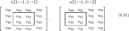
Slicing on the left side of line 2 in the above code selects the center subarray (boxed) from the left array in Eq. (6.91). It contains the interior points to be updated (compare with Figure 6.15). The boundary points where ui,j = 0 are excluded. The first term in the brackets on the right side of line 2 is depicted in the right array of Eq. (6.91). Here, slicing refers to the boxed subarray, which is shifted to the left by one column relative to the center box. Therefore, entries in u[1:-1,0:-2] are the left neighbors to u[1:-1,1:-1]. Similarly, the other three terms on the right side of the statement (lines 2 and 3) correspond to the right, top, and bottom neighbors, respectively. Here, left-to-right refers to moving across columns and top-to-bottom to running down the rows.
Through slicing and element-wise operations, the algorithm (6.90) is thus expressed succinctly in two compact statements. Because no explicit looping is used, computation is fast and highly efficient. We will encounter similar situations later and use the same technique (e.g., Program 6.8 and Section 7.2.1).
The results from Program 6.7 are shown in Figure 6.18 at several instants as contour plots and snapshots of the animated wave are shown in Figure 6.19. The initial wave is a product of symmetric Gaussians in both directions, localized at the center of the membrane (Figure 6.18, upper left). As time increases it spreads outward in the form of circular waves (Figure 6.18, upper right). It is rather like the ripple effect caused by a pebble hitting a water surface.
When the waves hit the boundary wall where the membrane is fixed, they are no longer circular. Instead, an inversion occurs, similar to that observed in waves on a string at the end points. But it is more complicated for 2D waves because the wavefront reaches the boundary at different times. The wavefront first hits the central portion of the walls (Figure 6.18, lower left). By the time it spreads toward the corner of the walls, the central portion has already inverted and started going toward the center (Figure 6.18, lower right). The wavefronts are distorted by the boundary walls.

After many encounters with the boundary, the wave develops numerous nodes and crests. It is thoroughly mixed, and the original Gaussian shape is unrecognizable. This is shown in Figure 6.19. Depending on the initial and boundary conditions, many interesting landscapes can occur, none repeating themselves, even after t ![]() L/v. For more explorations, see Project P6.8.
L/v. For more explorations, see Project P6.8.
Of course, to maintain stability of evolution, we must be sure the algorithm is stable. A value of β = 0.5 was used in generating the above results. For 2D waves, the range of stability of β is slightly different than for 1D waves. A von Neumann stability analysis can be carried out as discussed in Section 6.5.4. It is found that the FDM solutions are stable for ![]() . The number 2 under the square root comes as a result of two-dimensional space. Details are left to Exercise E6.8.
. The number 2 under the square root comes as a result of two-dimensional space. Details are left to Exercise E6.8.
6.8 A falling tablecloth toward equilibrium
The ideal waves on a membrane will oscillate forever. A realistic wave would suffer dissipation. We are interested in modeling such a realistic wave on a surface such as a tablecloth.
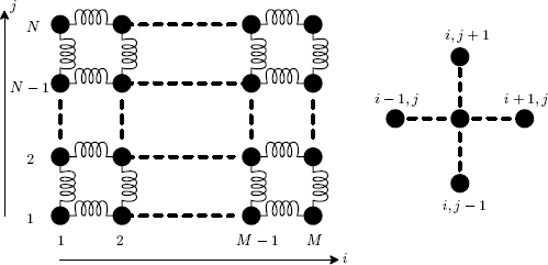
Figure 6.20: An array of particles on a grid. The right figure shows the nearest neighbor interactions.
We construct a tablecloth model as a two-dimensional array of particles arranged on a grid shown in Figure 6.20. There are N rows, and each row has M particles, for a total of M × N particles. Nearest neighbors are connected by springs. The particle at column i (x) and row j (y) interacts with its four nearest neighbors: left, right, top, and bottom. We assume initially the grid is laid out in the horizontal x-y plane. The force on the particle at (i, j) includes four spring forces plus gravity and damping as
![]()
The equations of motion for this system of particles are qualitatively the same as Eq. (S:6.5) (or (4.41) and (4.42) with Hooke's law), and can be solved accordingly. The included Program 6.8 closely mirrors Program S:6.2. It combines the numerical integration technique of Program S:6.2 and the visualization technique of Program 6.7. The visual representation of motion is based on dividing the particle grid (Figure 6.20) into triangular meshes, approximating a vibrating surface.
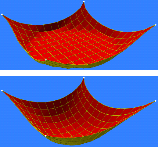
Program 6.8 can be used to simulate 2D waves with or without damping, for small or large amplitudes. It can also accommodate various types of boundary conditions, as well as constant or variable mass density with a slight modification. Figure 6.21 shows the results of a uniform surface (tablecloth) held at the corners and falling under its own weight. The tablecloth was initially flat and at rest. As it falls, it gains both kinetic energy and elastic potential energy. Toward the bottom, it rebounds, and oscillations start to propagate throughout the grid. Except the corner points, all the boundary points are free. For zero or small damping, very complex waves can be formed. After a while, the tablecloth settles into equilibrium. The overall shape is like the catenary (Figure S:6.1) spun around the central axis.
Our model can also be used to study relaxation time, rate of energy dissipation, boundary effects, etc. We will revisit the model for energy minimization in thermal physics (see Section 11.3).
Computationally, modeling a vibrating surface is much more expensive for a 2D particle array than for a 1D string. The core of Program 6.8 is cloth() which computes the forces in the equations of motion. If N is the linear dimension, the number of operations scales like N2 in 2D. For medium to large N, it would be a speed bottleneck for an interpretative language like Python if explicit looping were used (Section 1.3.2). But, like Program 6.7, cloth() uses implicit looping of NumPy arrays with efficient vectorized operations, enabling us to simulate 2D waves without the need of language extensions.
Programs 6.7 and 6.8 are prime examples where Python with NumPy provides the best of both worlds: the versatility and elegance of Python programming and the computational speed of compiled codes. Because this combination results in a flexible yet efficient workflow, use of NumPy (and SciPy) is indispensable in the chapters ahead. In most cases, this is sufficient. If extra speed boost is needed, we can turn to language extensions (see Program 5.7 for Mandelbrot fractals and Program S:11.4 for molecular dynamics).
Chapter summary
We began discussion of oscillations and waves with a damped, driven harmonic oscillator, including critical, over- and under-damping, and resonance. We discussed the oscillations of small systems such as triatomic molecules, its power spectrum, and normal modes motion. Reduction to linear systems of equations, eigenvalue problems, and their solutions are described using the SciPy linear algebra library.
The displacement of a string, representing the continuum limit of an array of particles under static forces, was discussed. The finite difference method (FDM) was applied to solving the displacement equation. We also introduced the basic idea of the finite element method (FEM) for 1D problems. In Chapters 7 and 9, we will extend the FEM to 2D problems in classical and quantum physics.
Simulations of one- and two-dimensional waves on a string and on a membrane as described by second-order PDEs were presented last. We discussed stability of solutions in terms of von Neumann stability conditions for the FDM scheme. We also presented a model using a grid of particles to approximate an oscillating membrane.
We have illustrated the use of several composite objects from the VPython modules (VPM) library to visualize oscillations and wave motion. The VPM library defines several classes of objects, including strings, slinkies, nets (grids), and meshes (triangular faces). These objects will be used in subsequent chapters.
6.9 Exercises and Projects
Exercises
| E6.1 | (a) Modify Program 6.1 so the oscillation is in the vertical direction. Do not forget gravity. How is the motion different from the horizontal case? Where is the equilibrium position? Explain.
(b) Show analytically that the only effect of gravity is to shift the equilibrium position of the oscillator. |
| E6.2 | Show that the RLC circuit in Figure 6.2 can be described by
Here q is the charge, ∈(t) the driving voltage. Find γ and ω0 in terms of resistance R, inductance L, and capacitance C. |
| E6.3 | The solutions to Eq. (6.1) may be obtained by assuming a trial solution of the form x(t) = exp(λt). Substitute it into Eq. (6.1) and solve the resulting characteristic equation for λ. Obtain Eq. (6.3) by a linear superposition of exp(λ±t) (see Sec. 8.5 of Ref. [10]). |
| E6.4 | (a) Assume a driving force of the form F = Fd exp(iωt), and a trial solution x = A(ω) exp(i(ωt + ϕ)) for Eq. (6.5). Show that A(ω) is proportional to Fd. (b) Verify the resonance condition (6.6) by finding the ωr for which A is maximum. |
| E6.5 | (a) Solve Eq. (6.18) for λ in the special case m1 = m3 = m and m2 = M. (b) Verify that if k = 1, m = 1/4, and M = 2/5, there are three eigenfrequencies ωi = 0, 2, and 3, i = 1 to 3. Remember λ = ω2. (c) Solve Eq. (6.13) for each ωi to obtain the eigenvector [ai1, ai2, ai3]. You will only be able to determine uniquely two of the three components. Normalize it such that the largest entry is unity. (d)* All of the above can be studied with SymPy as well. For example, factor Eq. (6.18) to show that zero is always a root (see Exercise E5.1). Next solve it symbolically for arbitrary masses. |
| E6.6 | (a) Program 6.5 shows the animated motion of the triatomic molecule in the symmetric vibration mode. Change the initial condition such that it represents the asymmetric vibrational motion.
(b) Start with an arbitrary initial condition, analyze the motion using the FFT method, and confirm the results in Figure 6.7. (c) Replace the Euler-Cromer method with the standard Euler method, and run the simulation again. What is the long-term consequence? |
| E6.7 | (a) Verify the FEM matrix Aij in Eq. (6.53).
(b) Evaluate pi given in Eq. (6.55) for linear and quadratic loads, f1 = a + bx and f2 = cx2, respectively. Express your results in terms of the node index i and grid spacing h. |
| E6.8 | Carry out a von Neumann stability analysis of the FDM equation (6.90) for waves in 2D to determine the stability condition for β = vΔt/h. |
| E6.9 | Starting from Eq. (6.68), derive the wavevectors for standing waves subject to one fixed end and one open end, Eq. (6.94). Do the same for two open ends. Sketch the first few standing waves in both cases. |
| E6.10 | Suppose a membrane is open on one side, say x = L. Derive the relation describing the open boundary condition in 2D. |
| E6.11 | We usually choose higher-order methods over lower-order ones, hoping to gain better accuracy and efficiency. Most of the time, it works out this way. However, higher-order methods are not always better. Strictly speaking, higher orders translate into better accuracy only if the problem is sufficiently smooth. For highly oscillatory problems like those we are dealing with in this chapter, a higher-order method can be worse than a lower-order one.
As an example, run Program 6.8 with the fourth-order Runge-Kutta RK4 and the fifth-order Runge-Kutta-Felhberg RK45n integrators. Observe the system's behavior with the latter. Is it physical? Vary the step size and watch where the problem starts, and analyze what caused the behavior (by plotting the energy of the problematic part, for example). Find ways to resolve the problem. |
Projects
| P6.1 | Consider the longitudinal oscillations of an N-particle array, Figure 6.22. Assume the interaction between neighboring particles obeys Hooke's law, and all the masses are the same.
(a) Set up the equations of motion for the system, and the A and B matrices as in Eq. (6.14). (b) Let N = 3, what kind of motion do you predict? Briefly write down your predictions. Integrate the equations with an ODE solver. Choose a suitable k and m, e.g., unity, and use an arbitrary initial condition, say u1 = 0.2, all others including velocities are zero. Optionally animate the motion of the particles with VPython. Plot the displacement of a particle as a function of time, u3(t), for instance. Discuss your results vs. predictions. (c) Obtain the power spectrum of the data plotted above. Identify the frequencies in the spectrum, remembering a ± frequency pair counts as one. Make sure you have enough data points which should be a power of two. Are the frequencies as you expected? Hint: To obtain a “clean” spectrum, adjust your step size so that the peaks are well separated and not “contaminated”. (d) Calculate the normal modes of the system. Compare the eigenfrequencies with your power spectrum results. Explain the motion associated with the normal modes. (e) Repeat the above calculations for N = 5. Identify all harmonics. Compare and discuss your results with the exact value, ωi = 2ω0 sin(iπ/(2N + 2)), i = 1, 2, …, N, where |
| P6.2 | Two coupled oscillators are shown in Figure 6.23. The horizontal oscillator (mass m1 and spring constant k) moves on a frictionless surface. A pendulum (mass m2 and cord length l) is connected to m1 via a cord.
(a) Show that the kinetic and potential energies are
(b) Take the small oscillation limit, expand T and V in powers of θ and retain terms only to second order in any combination of x, θ, (c) Let q1 = x and q2 = θ, and define
Compute the A and B matrices as
This is how A and B in Eq. (6.16) may be found for general small oscillations [40]. Calculate the eigenfrequencies and eigenvectors. Describe the normal modes. |
| P6.3 | This project and the next one (Project P6.4) should ideally be treated as team projects. Each individual team member can focus on one primary project, but work as a team exchanging ideas and results.
(a) Run Program 6.3 for the constant load f(x) = −2. Compare your results with Figure 6.11 (f = −1), and discuss the shapes of the strings. (b) Assume a linear load f(x) = −2x. Work out the exact solution from Eq. (6.29). (c) Modify your program to calculate the displacement numerically for the linear load. You need to change matrix B. Plot both numerical and analytical results. Compare each other and with Figure 6.11 for the linear case. (d) Predict what the shape will look like for a quadratic load, f(x) = −3x2. Sketch it. Carry out the FDM calculation. How did your prediction turn out? Explain. |
| P6.4 | Investigate FEM solutions for the displacement of a string under Dirichlet boundary conditions, u0 = uN = 0. It is helpful if you had gone through Project P6.3 individually or as a team.
(a) Modify Program 6.3 for the constant load, and make sure you can reproduce the FDM results shown in Figure 6.11. You can decide whether or not to move the factor h in Eq. (6.54) to the RHS of Eq. (6.52). Verify that doing so does not alter the solutions. (b) Consider the combination of constant and Dirac point-source loads shown in Figure 6.14. Reproduce the graphs. Your FEM program should be considered validated. (c) Calculate the displacement for the same linear and quadratic loads in Project P6.3. Results from Exercise E6.7 would be helpful. Compare the results. Plot the error between FDM and FEM solutions. Explain the discrepancy. |
| P6.5 | (a) Set up a traveling Gaussian wavepacket on a string. Do this by changing the initial condition in Program 6.4 to the following:
u1 = gaussian(x+h) or u1 = gaussian(x-h) Which would result in a right-traveling wave? Observe the actual wave. Is it a pure traveling wave? (b) Let us change u1 = gaussian(x+2*h). Predict the kind of wave that will be formed. Discuss the actual waves you see. (c) Figure 6.24 shows the second harmonic on the string. Implement initial conditions that will produce the standing wave, as well as the first, third, and fourth harmonics. |
| P6.6 | Study waves on a string with an open end. Suppose one end of the string is tied to a small, frictionless, massless ring that can move freely along a transverse thin rod at the boundary (say at x = L).
(a) By considering the balance of forces similar to Eqs. (6.26a) to (6.26b), show that an open end (or free) boundary is equivalent to
(b) Simulate waves on a string with a closed end and an open end. Modify the FDM scheme in Program 6.4 to take into account the boundary condition above and u0 = 0. Plot the waves as presented in Figure 6.16. What are the differences when one end is open? |
| P6.7 | Calculate the fundamental wavelengths of standing waves on a string with either one or two open ends.
(a) Assume only one open end, so the boundary condition is X(0) = 0, and ∂X/∂x|x=1 = 0. Implement the boundary condition to obtain the appropriate eigenequation analogous to Eq. (6.87). Plot the first four harmonics, discuss and compare your results to the exact values. (b) Repeat above for two open ends. |
| P6.8 | There are many more modes of oscillation with two-dimensional waves on a membrane. Let us sample a few of them.
(a) The waves shown in Figure 6.18 propagate outward from the center. Suppose we start the wave off center at (L/2, L/4). What do you expect the wave motion to be? Modify Program 6.7 and simulate this case. Describe your results. (b) What if the initial wave is asymmetric? Simulate this effect by introducing different Gaussian widths in the x and y directions. Which direction does the wave broaden faster? Why? (c) Is it possible to set up a pure traveling wave on a membrane equivalent to such a wave on a string (Project P6.5)? Make an educated guess. Test your hypothesis by changing u1 to a Gaussian (symmetric) displaced in the diagonal direction by a distance of v × dt relative to u0. Describe the resulting wave you see. Explain the wake. (d) What would standing waves look like in 2D? Set up a standing wave that is the first harmonic in the x direction and the second harmonic in the y direction. (e) So far we have assumed fixed boundary conditions. Now suppose we use periodic boundary conditions in the x direction, i.e., u(−h, y, t) = u(L, 0, t) and u(L + h, y, t) = u(0, y, t). Implement this boundary condition in your program. Discuss the differences with fixed boundary conditions. (f)* Simulate the waves on a membrane with an open boundary condition on one side, say at x = L. |
| P6.9 | Let us explore the falling tablecloth model in some detail.
(a) Study Program 6.8 to understand the organization of the code and the workings of the function cloth(). (b) Add a function that calculates the energy, E, of the system at a given time. The energy should include the kinetic and potential (elastic and gravitational) energies. Calculate the energy in the main loop, and plot it as a function of time for a given damping factor, say b = 0.2. Test that your code works correctly by checking some limits, e.g., without damping (b = 0 in Eq. (6.92)), the energy should be conserved. Find the final energy, Ef, when the system reaches equilibrium. Here equilibrium is defined as when the energy has reached a certain limit relative to the final energy, say 99%. Record the net energy loss as ΔE = Ei − Ef, where Ei is the initial energy. (c) Vary b from 0.1 to 1 in steps of 0.1. For each b, simulate the system until it reaches equilibrium. Record the time it takes for the system to lose half of the amount ΔE. Denote this time as the relaxation time. Plot the relaxation time as a function of b. Discuss your results. Can you classify the system in terms of under- and over-damping? For each b, also graph the change in energy (dE) as a function of energy difference E − Ef at each step. Characterize the trend between the rate of energy loss dE and E − Ef. Analyze the relationship between relaxation times and rate of energy loss. (d) Suppose we want to change the boundary condition. Instead of fixing only the corners, let us set the particles on opposite sides of the square fixed, e.g., at x = 0 and x = L. Predict how this will affect the relaxation time and the rate of energy loss. Change the boundary condition in cloth(), and run the simulation again. Compare the results with your predictions, and briefly explain. (e)* Currently, cloth() calculates the forces from the right and top neighbors directly, then uses the third law for the left and bottom neighbors (Figure 6.20). Re-code this function so the process is reversed, i.e., compute the forces from the latter directly, then apply 3rd law. |


6.A Program listings and descriptions
Program listing 6.5: Triatomic vibrations (triatom.py)
  1import visual as vp, numpy as np

  3def accel(u):
      return −k*np.array([u[0]−u[1], 2*u[1]−u[0]−u[2], u[2]−u[1]])/m
  5
col = [(1,0,0), (0,1,0), (0,0,1)]                # RGB colors
  7x0, atom, r = np.array([−3., 0., 3.]), [0]*3, 1.0
for i in range(3):
  9      atom[i] = vp.sphere(pos=(x0[i],0,0), radius=r, color=col[i])  # atoms
floor = vp.box(pos=(0, −1.1,0), length=8, height=0.2, width=4)     # floor
11s1 = vp.helix(pos=(x0[0],0,0), thickness=0.1, radius=0.5)            # spring
s2 = vp.helix(pos=(x0[1],0,0), thickness=0.1, radius=0.5)
13
h, k, m = 0.1, 1.0, np.array ([1./4, 2./5, 1./4])
15u, v = np.array ([−1.,0.,1.]), np.zeros(3)   # symmetric init cond
while True:
17       vp.rate(50)
       u = u + v*h                                        # Euler−Cromer method
19       v = v + accel(u)*h
       x = x0 + u
21       for i in range(3):                                # animation
             atom[i]. pos = (x[i],0,0)
23       s1. axis, s1.pos, s1.length= (1,0,0), x[0]+r, x[1]−x[0]−2*r   # move
       s2. axis, s2.pos, s2.length= (1,0,0), x[1]+r, x[2]−x[1]−2*r
Program 6.5 simulates the motion a triatomic system by solving Eq. (6.12) using the Euler-Cromer method. Other than dealing with three atoms, it works just like Program 6.1. The springs are attached to and moving with atoms 1 and 2 (line 23). They compress or stretch to fill the distances to their right neighbors, atoms 2 and 3, respectively.
Program listing 6.6: Standing waves on a string (stringfun.py)
This program computes the eigenvalues of the wavevector k2 on a string of unit length. After preparing matrix A the same way as in Program 6.3 using np.diag, it is scaled by −1/h2, such that the eigenvalues are actually for k2 instead of −h2k2. This is convenient since they will be positive and ordered in ascending order. Because this is a normal eigenvalue problem, matrix B is omitted from eigh().
The first four eigenvectors, stored in column i of u[:,i] for eigenvector i, are plotted with legends (mode number). As in Program 6.3, boundary values are inserted before plotting. To compare with analytical solutions directly, they are normalized at the first point from the boundary. A skip factor s is used to ensure that FDM symbols do not obscure the smooth analytical curves.
Program listing 6.7: Waves on a membrane (waves2d.py)
  1import numpy as np, visual as vp, vpm

  3def wave2d(u0, u1):
      u2 = 2*(1−b−b)*u1 − u0
  5      u2[1:−1,1:−1] += b*(u1[1:−1,0:−2] + u1[1:−1,2:]      # left, right
                                     + u1[0:−2,1:−1] + u1[2:,1:−1])    # top, bottom
  7      return u2
  9def gaussian(x):
      return np.exp(−(x−5)**2)
11
L, N = 10.0, 40        # length of square, number of intervals
13b = 0.25                   # betaˆ2

15x = np.linspace (0., L, N+1)                                    # mesh grid
x, y = np.meshgrid(x, x)
17u0, u1 = gaussian(x)*gaussian(y), gaussian(x)*gaussian(y)

19scene = vp.display(title =’2D waves’, background=(.2,.5,1),
                              center=(L/2,L/2,0), up=(0,0,1), forward=(1,2, −1))
21mesh = vpm.mesh(x, y, 2*u0, (.9,.8,0), (1,0,0))      # mesh

23while(True):
      vp.rate (40), vpm.wait(scene)                          # pause if key press
25      u2 = wave2d(u0, u1)
      u0, u1 = u1, u2                                                  # swap u’s
27      mesh.move(x, y, 2*u0)                                      # redraw mesh
The above code works in nearly the same way as Program 6.4. The only differences are that the arrays u0, u1, and u2 are two dimensional and the animation uses a mesh redrawn at each time step. The core function wave2d() relies on 2D slicing as described in Section 6.7. The VPM mesh object (line 21) is created with mesh(x,y,z, topcolor, bottomcolor) over the meshgrid (x,y) and displacement z. It is animated with the mesh.move() method (line 27).
Program listing 6.8: A falling tablecloth (tablecloth.py)
  1import ode, vpm, numpy as np, visual as vp

  3def force( r ):      # force of particle pair, with relative pos r
      s = np.sqrt(np.sum(r*r, axis=−1))                     # distance
  5      s3 = np.dstack((s, s, s))                                    # make (m,n,3) array
      return −spring_k*(1.0 − spring_l/s3)*r          # Hooke’s law
  7
def cloth(Y, t):     # tablecloth
  9       r, v, f = Y[0], Y[1], np.zeros((N,M,3))
11       rtop = r[0:−1, :] − r [1:, :]                           # rel pos to top neighbor
       rright = r [:, 0:−1] − r [:, 1:]                       # rel pos to right neighbor
13       ftop, fright = force(rtop), force ( rright )     # forces from top, right
       f[0:−1, :] = ftop                    # force from top
15       f [:, 0:−1] += fright               # force from right
       f [1:, :] −= ftop                     # below, left : use 3rd law
17       f [:, 1:] −= fright
       a = (f − damp*v)/mass + gvec
19       v [0,0], v[0, −1], v[−1,0], v[−1, −1]=0, 0, 0, 0   # fixed coners
       return np.array([v,a])
21
L, M, N = 2.0, 15, 15                           # size, (M,N) particle array
23h, mass, damp = 0.01, 0.004, 0.01       # keep damp between [.01,.1]
x, y = np.linspace(0,L,M), np.linspace(0,L,N)        # particle grid
25r, v = np.zeros((N,M,3)), np.zeros((N,M,3))
spring_k, spring_l = 50.0, x[1]−x[0]    # spring const., relaxed length
27r [:,:, 0], r [:,:, 1] = np.meshgrid(x,y)                      # initialize pos
Y, gvec = np.array([r, v]), np.array ([0,0, −9.8])     # [v,a], g vector
29
scene = vp.display(title =’Tablecloth’, background=(.2,.5,1),
31                               up=(0,0,1), center=(L/2,L/2, −L/4), forward=(1,2, −1))
vp.points(pos=[(0,0,0),(0, L,0),(L,L,0),(L, 0,0)], size=50)   # corners
33x, y, z = r [:,:,0], r [:,:,1], r [:,:,2]                                         # mesh points
net = vpm.net(x, y, z, vp.color.yellow, 0.005)                     # mesh net
35mesh = vpm.mesh(x, y, z, vp.color.red, vp.color.yellow)

37while (1):
      vp.rate(100), vpm.wait(scene)      # pause if key pressed
39      Y = ode.RK4(cloth, Y, 0, h)
      x, y, z = Y [0,:,:,0], Y [0,:,:,1], Y [0,:,:,2]
41      net.move(x, y, z), mesh.move(x, y, z)
We can use this program to simulate a falling tablecloth made of a 2D array of particles. The particles are initially arranged on a (M × N) grid (see Figure 6.20) but can move in 3D space. Like Program S:6.2 for 1D, neighboring particles interact through Hooke's force. The function force() computes this force given the relative position vector r between the particles. It first calculates the distance squared (line 4) by summing over the three components via np.sum along the last axis (i.e., x2 + y2 + z2), followed by the square-root. Because r is actually a 3D array (see below), the distance is a 2D array after the sum. Next the distance grid is stacked depth-wise with np.dstack (laying over each other) to form a 3D array, so that it has the correct shape for element-wise operations when multiplied by r to obtain the force (line 6). That is to say, every component of ![]() is divided by r3, akin to
is divided by r3, akin to ![]() , for every particle at once. We need to do this because automatic broadcasting is ambiguous here.
, for every particle at once. We need to do this because automatic broadcasting is ambiguous here.
The core function is cloth() which returns the equations of motion. The input Y=[r,v] contains the position r and velocity v vectors, respectively, each a (N, M, 3) array corresponding to the particles on the grid. Like Program 6.7, implicit looping via slicing is heavily used. For instance, we find the relative positions of the particles to the neighbors on top (one row above, Figure 6.20) by subtracting the rows shifted up by one from the current rows (line 11). The relative positions to the neighbors on the right can be obtained in a similar fashion. The forces can then be calculated from these relative positions and recorded accordingly (lines 14 and 15). We use Newton's third law (line 16) for the forces from the neighbors below and to the left, cutting the computational time by half. Note that slicing keeps the proper boundary conditions throughout. For example, the last column does not have neighbors to the right, so it is excluded correctly in f[:,0:-1] (line 15).
Once the forces are known, acceleration can be obtained for all particles at once. Finally, the velocities of the corner particles are set to zero (line 19), so they never move. The result is returned in a 4D array [v,a]. This again reaffirms the vector nature of our ODE solvers (Section 2.3.2) that can handle scalar (one ODE) and multidimensional vector equations automatically and transparently.
Visual representation of the tablecloth consists of a net overlaid onto a mesh. Like Program 6.7, we create a net with the VPM function net() which takes as input x, y, and z grid points, color, and thickness of the links. It is moved with net.move() as usual.
1The Millennium Bridge in London had to be closed just two days after opening in June, 2000 due to resonant swaying. The bridge swayed laterally when crowds walked over it, causing them to sway in step to keep balance, and leading to resonant vibrations. Fixed with more damping, it reopened 20 months later, nicknamed the “wobbly bridge”.
2The time and length scales are determined by the choice of units for k and mi. We can set them to arbitrary units without loss of generality. If they are in SI units, for example, then time and length would be in seconds and meters, respectively.
3This would be the case if the particles have the same, unity mass, and the couplings between them are neglected.
4You may also use SymPy's symbolic matrix manipulation to verify the results.
5The rotation matrix would be an N × N identity matrix except for rows i and j: aii = ajj = cosθ, aij = −aji = sinθ.
6Aside from efficiency derived from special algorithms for sparse matrices, we can also reduce memory bandwidth of the program, making it more efficient by minimizing the amount of data being moved, which may be as important as computational speed.
7We use the shorthand for x± = x ± ∈ where ∈ is a positive infinitesimal.
8For instance, the speed on the thickest string of a cello (C string) is v ~ 100 m/s. Assuming a mass density of ρ ~ 1.5 × 10⁻² kg/m for a metal string, the tension is T ~ 150 N, a strongly-strung string!
9The same phenomenon exists in quantum mechanics. See Section 9.6.2.