Chapter 7

Electromagnetic fields

In the simulation of few-body problems in Chapter 4, gravity was the sole interaction at large distances. If the particles are charged, they will interact via electromagnetic forces which are much stronger than gravity at the same distance. For example, the ratio of the Coulomb force to gravity between a proton and an electron is about 10³⁹ at a given separation, making gravity utterly negligible. In fact, macroscopic properties of all ordinary matter are determined by electromagnetic interactions. Forces such as tension in a string (Section 6.3), spring forces, friction, etc., are all manifestation of electromagnetic forces between atoms.

Like gravity, electromagnetic interactions occur through action at a distance via electromagnetic fields described by classical field equations, the Maxwell’s equations. In this chapter, we are interested in the simulation of electric potentials and fields in electrostatics and propagation of electromagnetic waves. Both scalar and vector fields in electromagnetism will be studied by solving the appropriate PDEs first encountered in Chapter 6. We discuss two mesh-based methods for solving the 2D Poisson and Laplace equations and related boundary value problems: an iterative self-consistent (relaxation) method, and a noniterative finite element method first introduced for 1D problems in Chapter 6. Complementing mesh-based methods, we introduce a meshfree method using radial basis functions for solving PDEs. Finally, we model the vector fields and electromagnetic radiation due to electric and magnetic dipoles.

7.1 The game of electric field hockey

Let us illustrate electric fields via a game of electric field hockey. The puck is electrically charged and moves in a rectangular playing area, the rink. Instead of contact forces by sticks involving a great number of atoms, Coulomb forces from stationary charges placed around the rink and at the center control the motion of the puck. A particular configuration of charges is illustrated in Figure 7.1.

The goal of the game is to score goals, of course. Two such goals are placed at the opposite ends of the rink. The rule of the game is simple: shoot the puck from one end with a given velocity; a point is awarded if it goes into the goal at the opposite end. If the puck goes out of bound, your turn ends.

Figure 7.1 shows three shots, two misses and one score. The success rate depends on the initial condition (skill) and the underlying physics for a given charge configuration. The configuration in Figure 7.1 consists of seven charges: five are positive, one at each corner and one at the center; two negative ones are placed in the middle of each side. In this example, the puck is negatively charged, so the forces on the puck are repulsive from the two negative charges on the sides and attractive from the corners and the center.

In the first instance, the puck was aimed at the lower side. When it got close to the negative charge, the repulsive force slowed it down, and turned it back up, resulting in a miss. The other instances had the same speed but different launching angles. In each case, the puck moved toward the center charge, orbiting around it once under its attractive force. The puck with the smaller angle suffered a greater pull, over rotated, and went out of bound from below, another miss. The third one had just the right pull, was catapulted toward the goal, and a score.

The hockey game simulator is given in Program 7.1. Most of the code is to set up visual animation. The actual game dynamics is modeled in hockey(), which returns the equations of motion as

where q is the charge of the puck, Q_i and the charge and position, respectively, of the stationary charges. The factor k = 1/4πε₀ = 9 × 10⁹ Nm²/C² is the electrostatic constant for the Coulomb force analogous to gravity (4.1). In the simulation, we set k/m = 1 for simplicity. This can always be done with a proper choice of units for charge and mass (Exercise E7.1).

The main program integrates the equations of motion (7.1), and checks whether the puck is in bound after each step. If it is out of bound, the code decides whether it is a miss or a goal.

As seen in Chapter 4 in the restricted three-body problem (Figure 4.17), the motion of the particle is more readily understood in terms of the potential surface it navigates on. Figure 7.2 shows the equipotential lines and forces (electric field) on the puck. The figure is plotted with Program 4.6 where the effective potential is replaced by the Coulomb potentials between the puck and stationary charges, (Project P7.1).

The five positive charges at the corners and the center act like sink holes the puck is attracted to. There are two saddle points, one on each side of the playing field, situated approximately in the middle of each half. Therefore, there is a minimum energy threshold for the puck to overcome the saddle point. Once over the threshold, the puck must navigate through the repulsive and attractive fields, and the trajectory can become very complex, as some in Figure 7.1 illustrate. This is true especially at lower energies when the puck must orbit around the center charge in order to escape to the other side. Occasionally, the particle can even become trapped to the center of the field, orbiting indefinitely. At higher energies, it is possible to deflect directly off the negative charge in the middle of the side and score a goal.

For the configuration of point charges considered here, it is straight forward to compute the potential surface and electric fields (forces) from Coulomb’s law. For other charge distributions (including continuous distributions) and arbitrary boundary conditions, we need to approach the problem differently. We discuss this next.

7.2 Electric potentials and fields

In electrostatics, Gauss’ law tells us that the electric flux through a closed surface is equal to the enclosed charge divided by a constant ε₀ (permittivity of free space). We can also express this law in a differential form using vector calculus. This differential form of Gauss’ law is called the Poisson equation [43],

where V is the electric potential, and ρ the charge density. The electric field can be obtained from V by

If the region within the boundary is charge free, i.e., ρ = 0 everywhere inside, Eq. (7.2) reduces to the Laplace equation. We are mainly interested in the two-dimensional Laplace equation,

Solutions to Eq. (7.4) are uniquely determined by the boundary conditions.

Like the displacement and wave equations discussed in Chapter 6, there are two types of boundary conditions: the Neumann and Dirichlet types. Under the Neumann boundary condition, the derivative, or more accurately the gradient, of V is specified on the boundary. This is equivalent to specifying the electric field on the boundary. On the other hand, the Dirichlet boundary condition deals with the values of V itself on the boundary. There can also be a mixture of both types of boundary conditions. Below, we will discuss solutions of Eq. (7.4) assuming Dirichlet boundary conditions where the values of V are given on the boundary points unless noted otherwise.

7.2.1 Self-consistent method

The general idea of self-consistent methods is to solve a given problem iteratively, starting from an initial guess. In each iteration, we use the previous iteration to obtain an improved solution. The process continues until the solution becomes self-consistent or relaxed toward the “equilibrium” value (see Section S:6.1.2 for the catenary problem solved with this method).

We will follow this approach here to solve the Laplace equation by relaxation. We shall first discretize Eq. (7.4), which is the same as the LHS of the wave equation (6.88). Accordingly, we can discretize the Laplacian over a 2D grid just like Eq. (6.89). Dropping the time variable from Eq. (6.90), the Laplace equation in FDM is

or equivalently,

As before, h is the grid size (we assume the same h for x and y), and we have used the following convention

Equation (7.6) states that the correct, self-consistent solution at any point is just the average of its four nearest neighbors. It is independent of the grid size h (though the accuracy is). Its simplicity is strikingly similar to Eq. (6.85) for an exact wave on a string.

Accordingly, if we find a solution satisfying Eq. (7.6) and the boundary condition, we have obtained the correct solution. So here is how the self-consistent method works: we start with an initial guess, say zero everywhere, and set the boundary values; then we go through every grid point not on the boundary, assigning the average of its four neighbors as its new value. In the beginning, we expect large changes in the grid values. But as the iterations progress, they should become more self-consistent, and only small changes will occur. We repeat the process until the solution has converged.

Program 7.2 implements this strategy (Section 7.A) to calculate the potential of two finite parallel plates kept at opposite potentials and placed inside a grounded box. The details of the program is described following the listing, but the central function is relax() below, which finds the self-consistent solution by relaxation.

  1 def relax(V, imax=200):            # find self−consistent soln
       for  i  in range(imax):
  3              V[1:−1,1:−1] = ( V[1:−1,:−2] + V[1:−1,2:]         # left,   right
                                       + V[:−2,1:−1] + V[2:,1:−1] )/4   # top, bottom
  5              V = set_boundary(V)    # enforce boundary condition
              draw_pot(V), vp.rate(1000)
  7        return V

The potential V is stored on a 2D grid as V [i, j] where, by convention of Eq. (7.7), indices i and j respectively refer to the x and y directions. The key statement is line 3. It uses the same slicing and element-wise operations as in 2D waves (see explanation in Section 6.7 and Eq. (6.91)) to compute the average of the four nearest neighbors, in remarkable resemblance to Eq. (7.6). Besides elegantly expressing the algorithm in one concise statement, we gain speed and efficiency since otherwise two nested loops would be required without implicit looping. Furthermore, the averaged values are assigned back to the same array without the need for a second array.

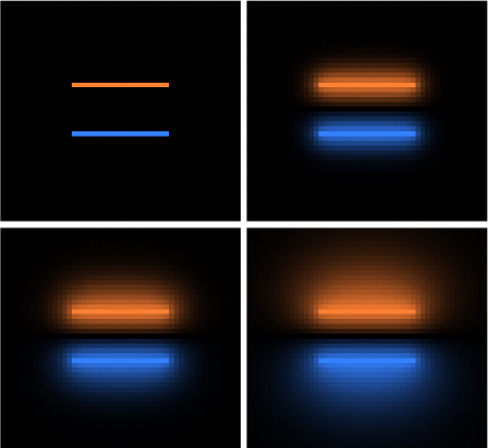
The statement is repeated many times, and the difference between iterations becomes progressively smaller. After each iteration, the boundary condition on the plates is applied, and the solution is visually displayed as colored points (Figure 7.3). Toward the end, very little change occurs, and we say the solution has become self-consistent, or it has converged. Finally, the potential and electric fields are plotted in 7.4. See Program 7.2 for the overall flow and explanation.

Figure 7.3 shows the progress of the solution as a function of iterations. At the start, the trial solution is set to zero everywhere except on the plates. After 20 iterations (top right), the potential has visibly spread to the immediate areas surrounding the plates. The outward spreading continues, although at a slower rate, as seen at iteration 60 (bottom left) and 200 (bottom right). After the last picture, it is hard to spot changes to the naked eye between iterations. But it is in fact surely getting closer and closer to the correct self-consistent solution, only too slowly (see below). This standard approach is known as the Jacobi scheme.

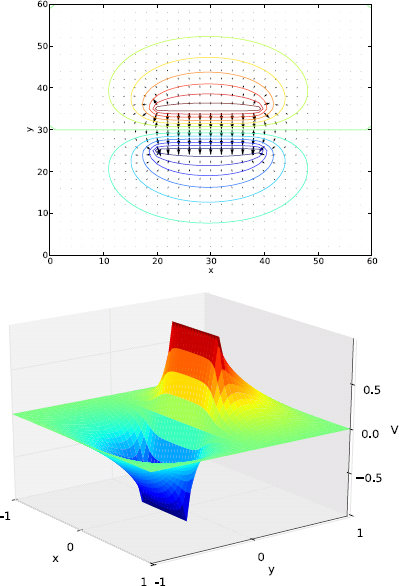
The potential contour lines plus electric field vectors and surface plots are shown in Figure 7.4. Constant contour lines of positive potential wrap around the top plate, and those of negative potential around the bottom plate as expected. In between the plates, we have approximately equidistant potential lines, consistent with the surface plot which shows a roughly linear slope inside as well.

Consequently, the electric field vector inside the plates is nearly constant, pointing from top to bottom. Near the edges, there are large fringe fields. Outside the plates, the “leaked” electric field is considerably weaker. In contrast, in the ideal case of infinite parallel plates, the electric field would be constant inside the plates and zero outside. The large fringe fields and nonzero fields outside are due to the plates being finite. They should become increasingly less significant if the plate size increases.

7.2.2 Accelerated relaxation

At first, we can see visual changes in the standard relaxation shown in Figure 7.3 because our initial guess, zero everywhere except on the two plates, is not close to the self-consistent (correct) solution. After a while, smaller changes occur with each iteration, the rate of convergence is rather slow. For instance, for the grid size used above (60×60), the solution is within a fraction of a percent of the correct solution in about the first 50 iterations. Thereafter, accuracy improves at a low power law (Figure 7.5). To gain one more significant digit, approximately 25 times more iterations are required. For larger grid sizes, the standard relaxation scheme is time consuming, and becomes impractical for calculations requiring higher accuracy. The root cause of the problem is that change at a particular grid point propagates slowly to neighbors far away, like in a diffusion process.

Another scheme, called the Gauss-Seidel (GS) method, makes the system relax faster. Instead of using only old values before the current iteration, the GS scheme uses the current values of the nearest neighbors as they become available in the current iteration. For example, if we start from the first row, and go across the column in each row, the modified loop in relax() in the GS scheme for one iteration would look like

for  i  in range(1, M−1):
       for j  in range(1, N−1):
             if  (not_on_plates( i, j )):
                   V1[i, j]=(V1[i−1,j] + V0[i+1,j] + V1[i,j−1] + V0[i,j+1])/4

Here, V0 is the old solution of the last iteration, and V1 the new solution. The function not_on_plates() checks that the point (i, j) is not on the plates (boundary) before updating. Because V1[i-1, j] and V1[i, j-1] (previous row and column of the current iteration) are available by the time the grid point (i, j) is being calculated, we make use of them. It mixes old and new values, and should converge faster. Indeed, it is faster than the Jacobi scheme by about a factor of two. However, its advantage does not stop there.

It turns out that the GS scheme is suitable for accelerated relaxation (successive overrelaxation) through the introduction of an acceleration parameter, α. Let V⁰ and V¹ be the values of the last (old) and current iterations, respectively. We can express the accelerated relaxation method as

If α = 1, we recover the Gauss-Seidel scheme. For α < 1, the process is under-relaxed, and usually results in slower convergence. Over-relaxation is achieved for α > 1, and generally speeds up the convergence. However, we must keep α < 2 as the method becomes unstable beyond 2. Even so, we need to be careful not to set α too close to 2, as it can cause fluctuations (noise) that do not vanish. For the grid sizes and geometries used here, we find it best to keep α ~ 1.85.

Figure 7.5 shows the average difference of the grid values between successive iterations, , which we take as a measure of absolute error in the solution. The error analysis was performed on the parallel plates system. The initial guess was the same as in the standard (Jacobi) and the accelerated GS methods.

At the beginning, the Jacobi method produced smaller differences than the accelerated GS method, presumably due to the mixing of old and new values in the latter. The slope of the error, however, is much steeper in the accelerated GS method. On the semilog scale, it is approximately a straight line, indicating a fast, exponential rate of convergence. Fully self-consistent solutions within machine accuracy are obtained in about 100 iterations. The standard relaxation method converges very slowly as a power scaling. The advantage of accelerated GS method producing accurate solutions efficiently is evident.¹

It is curious as to why the accelerated method works so efficiently. Physically, we imagine a situation analogous to the falling tablecloth (Section 6.8). The standard method would correspond to uninterferred relaxation into equilibrium, and the accelerated method to forced relaxation. The role of the parameter α can be thought of as an applied force, in addition to gravity, that pulls the tablecloth into equilibrium faster than gravity alone.

7.3 Laplace equation and finite element method

The self-consistent method solves the Laplace equation iteratively by successive relaxation. We can also solve it noniteratively with other methods. One such method is the finite element method (FEM) introduced in Chapter 6 for 1D problems. In this section we will extend the FEM to 2D in order to treat the Laplace equation. The FEM offers several advantages including easy adaptation to irregularly-shaped domains and accommodating different types of boundary conditions. More broadly, the FEM is widely used in science and engineering problems.

However, it takes some preparation to develop and understand the FEM framework. Hence, it is helpful to be familiar with 1D FEM first (Section 6.4), as our discussions follow a similar approach here in 2D.

The FEM development is organized in five steps:

• Choose the elements and basis functions;
• Set up meshes and tent functions for interpolation;
• Reduce the Laplace equation to integral form;
• Impose the boundary conditions;
• Build the linear system of equations (system matrix).

To see FEM in action first, you can skip ahead to Section 7.4 for a worked example and sample Program 7.3. You may also switch back and forth between FEM development and application.

7.3.1 Finite elements and basis functions in 2D

We wish to obtain the solution in a two-dimensional domain, a region surrounded by an arbitrary boundary. As in 1D, we expand the solution u in a basis set as

Analogous to Eq. (6.37), u_i is the expansion coefficient and ϕ_i the tent function to be formed with basis functions. Note that in 2D, we make a distinction between tent functions and basis functions for clarity.

In 1D, the basic elements were line segments, and the basis functions were linear functions between neighboring elements and zero elsewhere (Figure 6.12). In 2D, we can form a surface with a minimum of three points, so the simplest element is a triangle. We will divide the domain into triangular meshes, or elements. The vertices of the triangles are the nodes (we will use the terms nodes and vertices interchangeably in this section). Each node will belong to at least one element, but can belong to many more.

What basis function do we want to use over each element? Like the 1D case, the simplest function is a linear function in both x and y, which is an equation describing a plane. Since there are three nodes for each element, there will be three basis functions covering an element, one for each node.²

Sample basis functions are shown in Figure 7.6. Each basis function is a triangular plane defined to be unity at its own node and zero at the other two. The basis function is nonzero only over the element containing the node. It is defined to be zero outside the element (compact support).

Let the vertices of the triangle be (x_i, y_i), i = 1, 2, and 3. The basis function for node 1 can be written as [75]

The constant 2A is the magnitude of the cross product of the two vectors from vertex 1 to vertices 2 and 3, respectively, and is equal to twice the area of the triangle. We can verify that φ₁(x₁, y₁) = 1 and φ₁(x₂, y₂) = φ₁(x₃, y₃) = 0 at the nodes, and φ₁(x, y) = 0 along the base opposite node 1 (Figure 7.6, top left). The basis function φ₁(x, y) is the shaded triangular plane, which can be viewed as being formed by pulling one vertex of an elastic triangle up vertically, while holding the base down. Similarly, two other surfaces, φ₂(x, y) and φ₃(x, y), can be formed about nodes 2 and 3, respectively.

Let us denote the element by e. We label the nodes on element e as [1, 2, 3] in counterclockwise order. Also, let [i, j, k] represent a cyclic permutation of [1, 2, 3], including [2, 3, 1] and [3, 1, 2]. With these notations, we can generalize Eq. (7.10) to be

where A_e is the area of the element, same as A in Eq. (7.10).

Suppose we want to represent an arbitrary flat surface over element e. We can do so with a linear combination of the basis functions

This is illustrated in Figure 7.6 (bottom right). By varying the coefficients c_i, the patch can be stretched and oriented in any direction. Since our solution u(x, y) will ultimately be represented by the basis functions (through tent functions to be discussed below), u(x, y) will be composed of flat, triangular patches over the domain.

7.3.2 Meshes, tent functions and interpolation

We illustrate with an example how the meshes, basis functions, and the tent functions fit together. Figure 7.7 shows a ¬-shaped domain, a rectangle with a missing corner. We divide it into four elements (meshes), numbered from e₁ to e₄. There are six nodes in total, all on the boundary. Node 1 is a member of all four elements, nodes 2 and 6 of a single element, and nodes 3 to 5 of two elements.

We associate a tent function with each node for interpolation as given by Eq. (7.9). A tent function is just a collection of basis functions from all elements containing the node. Two tent functions are drawn in Figure 7.8.

The first tent function at node 1 consists of four basis functions since node 1 belongs to all four elements. This tent function would be closed except for the fact that the node is on the boundary, and the lower-left corner is therefore open. We can express this tent function in terms of the basis functions as

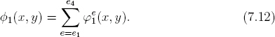
The tent function is continuous, though not smooth, across the element boundaries (the ridges). Because the basis functions are zero outside their own element boundaries, the value of ϕ₁ at a given point (x, y) can be found on one, and one only, basis function of the element containing that point.

This is true for all points except those on the ridges and the exact node point for which the tent function is defined. To avoid double counting, we require that only one term in the sum (7.12) is actually selected: the basis function of the first element determined to contain the point. The value of the tent function at the node is unity by definition.

Likewise, tent functions at other nodes can be built in the same way. For example, the tent function at node 3 (Figure 7.8, bottom) has two basis functions, one each from elements e₁ and e₂. There are six such tent functions, one for each node. We note that two tent functions overlap each other only if the two nodes are directly connected by an edge. For instance, the two tent function shown in Figure 7.8 overlap because nodes 1 and 3 are connected by the common edge between e₁ and e₂. In contrast, the tent functions at node 3 and node 5 would not overlap.

Suppose we are given the values of a function at the nodes u_i, and we wish to interpolate the function over the whole domain. Then from Eq. (7.9), we just need to run the sum over all the tent functions thus defined.

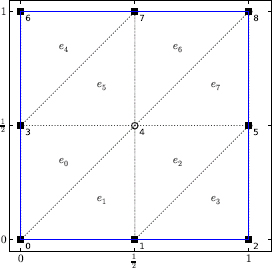
To see it in action, we show the interpolation of the function f(x, y) = sin(πx) sin(πy) over the unit square in Figure 7.9. The meshes are shown in the left panel, and the function (wireframe) and its interpolations (solid pyramids) in the right panel.

Two different sets of meshes are used. In the first instance, the domain is divided into eight elements, with one internal node and eight boundary nodes. The values of u_i = f(x_i, y_i) are zero at the boundary nodes and 1 at the lone internal node (the center). Of the nine tent functions, only the one at the center contributes. The interpolation is therefore given by this tent function which is a six-sided pyramid. The front and back facets have been sliced off because all node values of elements e₄ and e₅ are zero. The interpolation is below the actual function over most of the domain, except at the other two edges along the diagonal (between e₁/e₂ and e₇/e₈).

The second set (Figure 7.9, second row) increases the number of meshes to 18. Now there are four internal nodes with the same value . Summing up the four tent functions gives us a flat-top pyramid. Again the front and back edges corresponding to elements e₆ and e₁₃ are sliced off, but by a smaller amount than before. There are no improvements over the other two edges. However, overall fill volume has improved, mainly due to the facets becoming closer to the function.

We mention two observations. First, if we increase the number of meshes to make them finer, the interpolation would become better. However, one thing remains: the interpolation is made up of flat, finite patches that are continuous across element boundaries, but their derivatives are discontinuous.³ Second, the way we have divided the domain up along one diagonal of the unit square breaks some symmetries of the original function. This impacts the quality of the interpolation and of the solution when symmetries are important in a problem. Mesh generation should take these factors into account.

7.3.3 Reduction to a linear system of equations

Because the gradient of the FEM interpolation is discontinuous across element boundaries, we cannot work directly with second-order equations like the Laplace equation in differential form. Rather, like in 1D, we convert the problem into one involving only first derivatives.

Let us consider the Poisson equation in 2D (change V to u in Eq. (7.2)),

where σ is the surface charge density. Similar to Eq. (6.42), we multiply both sides of Eq. (7.13) by ϕ_j(x, y) and integrate over the domain S as

Using the identity v∇²u = ∇ · (v∇u)−∇v · ∇u, we can reduce Eq. (7.14) to

The first term can be simplified with Green’s theorem, which converts a surface integral of divergence over S into a line integral along the boundary C

The contour of integration C encloses the domain S in the counterclockwise direction, and the normal vector points outward and perpendicular to the tangent of the contour [10].

With the help of Eq. (7.16), we can rewrite Eq. (7.15) as

Note that for the Laplace equation, f(x, y) = 0, so p_j = 0, but we keep it for generality. We substitute the interpolation (7.9) into (7.17) to arrive at

Let

we can express Eq. (7.18) for each node j as

This is a linear system of equations, to be solved subject to boundary conditions.

7.3.4 Imposing boundary conditions

We can specify two types of boundary conditions in Poisson (or Laplace) problems: the values of the electric field, ∇u (Neumann type), or the values of the potential, u (Dirichlet type). Using two parallel plates as an example, the Neumann type would correspond to specifying the electric field on the plates (analogous to setting up surface charge densities), and the Dirichlet type to keeping the plates at certain voltages. We are mostly interested in the latter here, and restrict our discussion below to Dirichlet boundary values.

Suppose node k is on the boundary with a given value u_k. Since this node no longer needs to be solved for, we remove the kth equation from Eq. (7.20), and move the term A_jku_k(j ≠ k) in other equations to the RHS so the new system is

We have one fewer equation in (7.21) than (7.20).

We can eliminate all other boundary nodes the same way, crossing off the equations corresponding to these nodes and moving them to the RHS in the rest, so we end up with

The sums on the LHS and the RHS involve internal and boundary nodes only, respectively.

There is one more simplification we can make. Because the index j in Eq. (7.22) runs over internal nodes only, and the tent function centered on an internal node is zero on the boundary (see Figure 7.8 and discussion following it), q_j as given in Eq. (7.17) is zero since the line integral is on the boundary where ϕ_j = 0. Therefore, we can drop q_j from Eq. (7.22). This is an expected result since we are concerned with the Dirichlet boundary condition here, and q_j involves the Neumann type (∇u on the boundary).

Expressing Eq. (7.22) in matrix form, we have

It is understood that indices of the matrix entries refer to the internal nodes. This is the final FEM result. Solving Eq. (7.23) will give us the FEM solutions uniquely determined by the boundary condition. For the Laplace equation, we can also drop p_j’s from Eq. (7.23), leaving only b_j's.

7.3.5 Building the system matrix

The matrix entries A_ij in Eq. (7.19) involve the gradient of the tent functions ϕ_i and ϕ_j which are composed of basis functions. The evaluation of A_ij will necessarily operate on the basis functions of the elements containing the nodes i and j.

To make this explicit, let us denote the list of elements connected to node i by e(i). For example, referring to Figure 7.7, four elements contain node 1, so the list for node 1 is e(1) = {e₁, e₂, e₃, e₄}; and for node 2, e(2) = {e₁}, etc.

Similar to Eq. (7.12), the tent functions ϕ_i and ϕ_j can be written as

where the basis functions are given in Eq. (7.11). Substitution of ϕ_i and ϕ_j into Eq. (7.19) yields

This result tells us that only basis functions in the elements containing nodes i and j contribute to A_ij. Furthermore, because a basis function is zero outside its own element, there will be no contribution to A_ij unless e(i) and e(j) refer to the same element. In other words, A_ij will be zero unless nodes i and j are directly connected.

It seems that a straightforward way to calculate A_ij is to proceed as follows. For each node, we build a list containing the elements the node belongs to. When evaluating the sum in Eq. (7.25), we just go through the lists associated with the pair of nodes. But this node-oriented approach would be cumbersome and inelegant. For instance, additional bookkeeping would be necessary to decide whether a pair of nodes are directly connected, as well as what the common edges are.

A more natural way is the element-oriented approach. We specify each element by listing the three nodes at its vertices (in counterclockwise order). Then, we iterate through the elements, computing the contributions from each element (e = [i, j, k]) to the six entries of matrix A: three diagonals and three off-diagonals plus the symmetric pairs , etc. After iterating over all the elements, all contributions will have been accounted for, and the matrix A will be completely built.

Let us illustrate the element-oriented approach using the mesh shown in Figure 7.7 and reproduced in Figure 7.10. The six nodes are numbered 1 to 6 and have coordinates (x_i, y_i), i = 1 to 6. The four finite elements are specified as e₁ = [1, 2, 3], e₂ = [1, 3, 4], etc. Let

This is the contribution to A_ij from element e. It is symmetric about the diagonal, . Note that we have changed the integration domain S to S_e, the domain over element e.

Figure 7.10 shows the contributions to off-diagonal entries of matrix A. We start from e₁ with nodes [1, 2, 3]. It contributes to matrix A along the three edges as , and . There are also symmetric pairs , etc.) and diagonal entries (e.g., , not shown in Figure 7.10).

After e₁ has been processed, entries A₁₂ and A₂₃ and their symmetric pairs are complete. No contributions will come from other elements (besides e₁) because node 2 is connected only to nodes 1 and 3. By the same token, after processing e₂, all entries associated with e₁ (plus A₃₄ with e₂) are complete with the exception of A₁₁ which awaits further contribution from elements e₃ and e₄. For example, the entry A₁₃ will be complete to become . We see that after going through every element, all entries of matrix A will be complete.

We can accomplish the matrix-building process with the following pseudo code:

for e in [e₁, e₂, e₃, e₄]: for m = 0,1,2: for n = m to 2: i = e[m], j = e[n] A_ij = A_ij + from (7.27) if i ≠ j: A_ij = A_ji

The two inner loops cycle through the nodes of a given element, assigning the contribution to the appropriate entry of A, and taking advantage of symmetry about the diagonal.

It is now just a matter of evaluating Eq. (7.26) to complete the construction of matrix A. The gradient may be obtained from Eq. (7.11) as , which is a constant vector over element e. Therefore, Eq. (7.26) becomes

Once matrix A is prepared, the linear system (7.23) is readily solved.

7.3.6 Mesh generation

Mesh generation is a major effort in FEM. The quality of the mesh can affect the quality of solutions and computational efficiency. There are special Python packages dedicated to just mesh generation. We will discuss the basic idea and the data structure in the generation of triangular meshes.

Let us consider a rectangular domain shown in Figure 7.11, over which the Laplace equation is to be solved. We divide the domain into N intervals along the x-axis and M intervals along the y-axis. The grid will have N×M sub-rectangles and (N + 1) × (M + 1) grid points, i.e., nodes. Each sub-rectangle is subdivided into two triangles along the diagonal. Each triangle is a finite element, so there are a total of 2N × M elements. Figure 7.11 shows a mesh grid where the unit square is divided with N = M = 3. There are 16 nodes (consecutively numbered), including 12 boundary nodes and 4 internal nodes, and 18 elements.

We store the nodes as a master list of coordinates (n × 2 array). The elements are also stored in a list, each entry having three numbers: the indices of the nodes (vertices) in counterclockwise order. The boundary and internal nodes are indexed to the master list as well. Table 7.1 illustrates these variables and sample values.

A node may belong to several elements, e.g., node 5 is a member of six elements, e_0−2,7−9. The coordinates of an element’s vertices may be determined by finding the indices associated with the nodes. For example, the second vertex of the first element e₀ is node elm[0][1]=5, and the coordinates are node[elm[0][1]], or from Table 7.1 and Figure 7.11. See Figure 9.24 for another sample mesh.

With the sample mesh of Figure 7.11, the dimension of the full matrix is 16 × 16. After removing the boundary nodes, the actual linear system (7.23) to be solved would be 4 × 4. As we will see next, the matrix is banded (Figure 7.12), and most entries are zero (see Project P7.5).

7.4 Boundary value problems with FEM

7.4.1 A worked example

We present a worked example of boundary value problems with FEM as applied to the Laplace equation over a rectangular domain. We assume a unit square such as the one shown in Figure 7.11. The boundary conditions are that the potential is zero on the left and bottom sides, and a quadratic curve on the right and top sides. They are (we make a notation change from V to u to be consistent with the FEM development)

The FEM program designed to solve the Laplace problem with these boundary conditions is given in full in Section 7.A (Program 7.3). The program has two key parts: mesh generation and system-matrix construction.

Mesh generation is discussed in detail following the program. The construction of matrix A is done as follows.

The routine goes through the element list elm. For each element, the coordinates of the vertices are extracted from the node list, and the parameters β₀₋₂, γ₀₋₂ and A_e are calculated according to Eq. (7.11). The contributions to matrix A, , where m and n are the nodes of the current element, are computed from Eq. (7.27). Three of the six off-diagonal entries are computed, the other three are obtained via symmetry.

We show in Figure 7.12 a sample system matrix with N = 10. The boundary points have been removed, leaving the matrix dimension at 81 × 81. The matrix is sparse, consisting of three bands. We expect a sparse matrix, since A_ij is nonzero only if the nodes i and j share a common edge (directly connected). From Figure 7.11, we see a node has a maximum of seven connections (six neighboring nodes plus self). However, Figure 7.12 shows that a row (or column) has at most five nonzero entries, two less than the number of connections.

The reason turns out to be that our finite elements are all right triangles. As such, the entries A_ij on the hypotenuse are zero. Take node 5 in Figure 7.11 as an example, A_5,0 and A_5,10 are zero. We can visualize that the basis function at node 5, , changes along the x direction only; while the basis function at node 0, , changes along the y direction only; such that their gradients are perpendicular to each other, resulting in zero contribution to A_5,0. The same reason applies to contributions to A_5,0 from e₁ and contributions to A_5,10 from e₈ and e₉.

The sparseness of the matrix means that the number of nonzero matrix entries scales linearly with N², rather than N⁴. With special storage schemes, we could deal with a large number of finite elements before running out of memory (see Section 8.3.1 for band matrix representation).

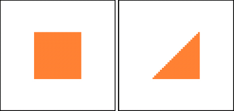
We have the necessary ingredients to solve for the potential values at the internal nodes. The rest of Program 7.3 is described following its listing. We show the results in Figure 7.13. The potential slopes down monotonically from its highest point at (1, 1), and is symmetric about the ridge running down the diagonal line to the origin. The slope is greatest near the top, producing the greatest electric fields there (arrows on the contour plot).

The electric field near the top and right sides initially points away from the sides near the highest point. Further left and down, it becomes weaker and its directions turn toward each side. By the midpoint, they are parallel to the respective sides, but eventually point into the sides past the midpoint. On the left and bottom sides, however, the electric fields are perpendicular to the boundaries because the potentials are constant on these sides. As the contour lines extend closer to the bottom-left corner, they start to mimic the shape of the walls, running nearly parallel to them and bending more sharply near the origin.

To approximate the solution near the corner more accurately, finer meshes would be necessary. How fine? The answer lies in the accuracy of FEM solutions considered next.

7.4.2 Accuracy and error of FEM solutions

To analyze the accuracy and error of FEM solutions, we consider an example which admits compact analytic solutions. We assume the same unit-square domain as in the worked example above but with sinusoidal boundary conditions as

The analytic solution can be shown to be

We only need to change the mesh() routine slightly to take into account the new boundary conditions to obtain the FEM solutions from Program 7.3. The results are displayed in Figure 7.14.

The boundary conditions dictate that the solutions be zero at all four corners. Because of this, there is a saddle point in the potential surface near where the potential shows considerable variation, in contrast to the monotonic solutions of Figure 7.13. The contour lines as well as electric fields (not shown in Figure 7.14) show symmetry about the diagonal line y = x. Away from the saddle point and toward the left and bottom sides, the potential distribution approaches the boundary values, a situation similar to that in Figure 7.13.

To assess the accuracy of FEM, we show in Figure 7.15 the absolute difference between the analytic and FEM solutions (Project P7.6). At each node, we compute the difference as

where u_exact is the analytic solution (7.30), and u_FEM the FEM solution (Figure 7.14). The parameter N = 40 is used in the FEM calculation, corresponding to grid spacing of 0.025, and 3, 200 finite elements. The error is displayed as a color-coded image using plt.imshow() (see Program 7.4).

The difference ranges between 0 and ~ 3×10⁻⁴, and is always positive. The FEM results are consistently below the analytic ones, even though the solution is not monotonic as discussed above. The smallest error occurs near the boundary as expected. The largest error is slightly off the saddle point where the potential values are largest away from the boundaries.

In Figure 7.16, we show the average error of the FEM solutions as a function of N. The error decreases with increasing N, but the slope after the second point (N = 4) is a straight line. Since the plot is on a log-log scale, it indicates that the error decreases as a power law. Careful examination of the trend shows that the slope is −2, or error ~ N⁻². Doubling N reduces the error by a factor of 4.

Since the grid spacing h ~ 1/N, we conclude that FEM with triangular meshes is second order in accuracy, the same as FDM. In hind sight, we probably could have guessed this, because the linear interpolation in FEM is like the trapezoid rule, which is also second order (Section 8.A.1). Higher order polynomial basis functions could also be used, but the resulting system matrix would be more complex [38].

7.5 Meshfree methods for potentials and fields

The methods we have discussed so far all involve certain ways of discretizing space into grids or meshes, over which the differential operators are approximated. The accuracy of mesh-based methods can generally be improved by reducing the mesh size h.

There is another class of meshfree methods taking a different approach. Rather than discretizing space, the solutions are interpolated over a chosen set of basis functions. We discuss one meshfree method here, namely, the radial basis function method.⁴ The advantage of this method is that it is fast, straightforward to implement, and can easily handle irregular domains. It may also be readily scaled up to higher dimensions. The drawback is that its accuracy depends on the quality and size of the basis set, and it is trickier to systematically improve accuracy.

7.5.1 Radial basis function interpolation

The basic idea of meshfree methods is scattered data interpolation [96]. We assume that, like in FEM, the solution u can be approximated by expansion in a distance-based radial basis function (RBF) set as

where a_i are the expansion coefficients.

There are many possible functional forms for ϕ_i. We cite two commonly used RBFs as example, the Gaussian (GA) and the multiquadric (MQ),

where ε is the shape (control) parameter, and are the nodes (centers) scattered over the domain of interest.

We can use Eq. (7.31) for scattered data interpolation (Figure 7.17). For example, suppose we have four known data points, u_i at to 4. The scattered data points are not restricted to any particular geometry. The coefficients a_i can be determined by requiring

where we have taken the nodes to coincide with the scattered data points. The result can be expressed as a matrix equation

Equation (7.34) can be solved for the RBF expansion coefficients a₁₋₄. The matrix entries are defined at the RBF collocation points as

where ϕ is either a GA or MQ RBF in Eq. (7.32). Because the RBFs are based on the radial distance from the nodes, the system matrix is positive and definite. Furthermore, its determinant is invariant under the exchange of any pair of nodes because the scalar distances r_ij remain the same. Therefore, the system matrix is well-conditioned, and the solution is assured to be nonsingular (Exercise E7.6). In fact, the tent basis functions in the 1D FEM (Figure 6.12, Eq. (6.38)) are linear RBFs, and share some of above traits, except they are not infinitely differentiable like the GA or MQ. In general, however, if the basis functions were position (rather than distance) based, the above mentioned properties would no longer hold. In this respect, scattered data interpolation by RBFs has unique advantages.

Figure 7.17 illustrates an example consisting of four Gaussian RBFs centered at the scattered data points. After obtaining the expansion coefficients a₁₋₄ (vertical lines at the nodes in Figure 7.17, left), the resultant interpolant (7.31) can be used to approximate the solution over the whole domain.

7.5.2 RBF collocation method

The RBF collocation method is a way to solve PDEs. It is based on differentiating a RBF interpolant, from which the differentiation operator matrices can be built [27]. As an example, we use the method to solve the 2D Poisson equation with the Gaussian RBF (equally applicable to 3D).

We consider a region surrounded by an arbitrary boundary (the domain). Let N be the total number of scattered nodes. Of these, we assume the number of internal nodes is n, and the number of boundary nodes is N −n.

Substituting the interpolant (7.31) into the Poisson equation (7.13), we obtain

The collocation method, also known as Kansa’s method [52], stipulates that the Poisson equation (7.36) be satisfied at the internal nodes , j ∈ [1, n], and simultaneously, the boundary conditions be also satisfied at the boundary nodes , j ∈ [n + 1, N].

For simplicity, we assume Dirichlet boundary conditions. We have for the collocation method

where , and b_j are the potential values on the boundary. Casting Eqs. (7.37a) and (7.37b) into matrix form, we have

where a = [a₁, a₂,…, a_N]^T is a column vector to be determined, and

The differentiation operators and RBF values are defined as

The system matrix A is square but asymmetric. It can be evaluated given the specific RBF (GA or MQ) and the nodes. If the operator is different than the Laplacian, it can be modified in a straightforward way. The vector b consists of the charge densities f_j and the boundary values b_j. Once the necessary parameters are known, we can obtain the solutions a by solving Eq. (7.38) in the same manner as Eq. (7.23).

Let us apply the RBF collocation method to solve the Laplace equation with Gaussian RBFs. The system geometry is a disk (roughly an octagon at the current node spacing) in the center of a square box, Figure 7.18. We assume the box is kept at zero potential and the disk at a constant potential (say 1). We simply distribute the nodes uniformly over the domain (23×23), though other choices are also possible (e.g., the Halton sequence [27]). The number of internal nodes is n = 344, and the number of boundary nodes is N − n = 185. The b vector in (7.39) consists of zeros in the top n rows and ones in the bottom N − n rows.

The required differentiation operator is (Exercise E7.6)

It can be readily evaluated to form the system matrix A given the nodes and the shape parameter ε. The value of ε turns out to be critical to the accuracy and success of the RBF method. It is known that the accuracy depends on ε, sometimes very sensitively, given the choice of the RBF type and the placement of the nodes [55]. Typically, the extreme values, either very small or very large ε, lead to very bad approximations. It is unknown, however, where the sweet spot is in general. Sometimes we must find it by trial and error. From the applied physicists’ perspective, we resort to physics to guide us, e.g., Eq. (6.82). Suppose h is the typical distance between the nodes. We expect that the resolution should be such that εh ~ 1, or ε ~ 1/h.

Figure 7.19 shows the results of the RBF collocation method from Program 7.4. It is structurally similar to the FEM code and is fully explained in Section 7.A. The value ε = 20 is used (the actual spacing is 1/22). However, test shows that values from ~ 10 to 25 works as well. The potential is highest, and approximately constant, within the disk (or the octagon), and decreases to zero toward the walls as expected. It also shows the correct symmetry for the configuration.

Compared to FDM, the accuracy of the RBF method is good (Project P7.9). Considering that sharp corners usually require higher density of nodes for the scattered data interpolation to be accurate, the RBF results with a modest number of uniform nodes in the present case are satisfactory. The RBF method is fast, and easier to use than the FEM. The disadvantage is that it is more subtle to control accuracy systematically.

With FDM or FEM, we can progressively reduce the error with smaller meshes (within the limits of machine accuracy or memory). In the RBF method, we expect that increasing the number of nodes will lead to more accurate results. However, if the number of nodes changes, we need to change the shape parameter accordingly, whose optimal value is not known a priori. And the situation may be different for different RBFs (Project P7.9).

Finally, the location of the nodes may represent a potential degree of freedom that can be exploited to our advantage, similar to the location of the abscissa in Gaussian integration (Section 8.A.3). For instance, it is thought that some other independent way (equilibrium points, standing wave nodes, etc.) may foretell a set of good nodes from bad ones, proof again that sometimes numerical computing is indeed a form of art.

7.6 Visualization of electromagnetic fields

We have discussed electrostatic problems where the electric charges are stationary. In this section we are interested in visualization of electromagnetic vector fields produced by either steadily moving charges or accelerating charges. The vector fields can be effectively visualized using the tools and techniques we have employed so far.

7.6.1 Magnetic fields due to currents

In magnetostatics, the source of magnetic fields is moving charges, i.e., electric currents. Like Coulomb’s law for electric fields, the Biot-Savart law describes the magnetic fields due to a current segment as

where I is the current, the current-carrying line segment (Figure 7.20), the position vector relative to , and μ₀/4π = 10⁻⁷ T·m/A. The total magnetic field is the sum over all segments, and for a continuous current distribution such as shown in Figure 7.20, it approaches a line integral.

As a first example, we simulate the magnetic field of a closed loop. We consider the loop as a unit circle placed in the x-y plane, forming a magnetic dipole.⁵

Figure 7.21 displays the magnetic fields calculated from Eq. (7.42) in Program 7.5 using 36 circular segments. Because it is rotationally symmetric about the z-axis, we show a cut of the field in the x-z plane, perpendicular to the loop. The current comes out of the page in the left eye in Figure 7.21 and goes into the page in the right eye. The magnetic field is strongest inside the loop (between the eyes), and weakens significantly outside it. This is because the magnetic fields from all line segments are additive inside, but are canceling outside due to the vector product nature of Eq. (7.42). Along the central z-axis, the magnetic field is perpendicular to the loop.

3D vector field visualization

By swinging around the central z-axis in Figure 7.21, we could imagine how the magnetic fields look like in 3D. But they can also be directly visualized using VPython. This can give a new perspective to viewing vector fields. Figure 7.22 shows two 3D examples of the magnetic fields of a dipole and of a long, current-carrying wire.

For the dipole, the calculation of the magnetic fields remains the same and only the representation is different. To preserve symmetry, the spatial points are chosen in a axially symmetric manner (see Program 7.6).

For the long, current-carrying wire, we use the analytic results for the magnetic fields,

The direction of the current is out of the page, so the magnetic fields are in counterclockwise tangential directions as given by the right-hand rule. In both examples, we can rotate the scene to view the fields from arbitrary viewpoints.

7.6.2 Electromagnetic radiation of an oscillating dipole

In electrodynamics, if moving charges are also accelerating, e.g., moving along a curved path or oscillating back and forth, they emit electromagnetic radiation. One of the most important sources of radiation is an oscillating electric dipole. This can be thought of as a pair of opposite charges oscillating sinusoidally about their center. Let us assume the center at the origin and the oscillation in the z direction. The electric dipole may be written as

where p₀ is the magnitude of the electric dipole, and ω the angular frequency. The resulting electromagnetic fields in 3D visualization obtained from Program 7.7 are shown in Figure 7.23.

A way from the dipole in the radiation zone (kr 1), the electromagnetic fields have particularly simple expressions [50],

Here c is the speed of light, k = ω/c = 2π/λ the wavevector (λ the wavelength).

The magnitudes of the electromagnetic fields decrease inversely proportional to r. This ensures that the radiative power, proportional to , is constant through a spherical surface on average.⁶ This is in contrast to electrostatic dipole electric fields which fall off much faster at 1/r³ at large distances.

On the spherical surface of a given radius r, the magnitudes vary as B, E ∝ sin θ, with θ being the polar angle (see Figure 7.20). Therefore, the radiation is anisotropic and highly directional. Figure 7.24 shows the angular distribution of field magnitudes from Program 7.8.

The pattern displayed in Figure 7.24 is characteristic of a dipole distribution. The fields are zero at the north and south poles along the dipole axis (θ = 0 and π), and maximum at the equator. Furthermore, as Figure 7.23 shows, the electric field is longitudinal and magnetic field latitudinal, such that they are perpendicular to each other at a given point. Their cross product is along the radial vector, the direction of field propagation. As a result, the radiative power is largest near the equator in the direction perpendicular to the electric dipole.

Plane electromagnetic waves

As seen above, the electric and magnetic fields in free space are perpendicular to each other, with the direction of propagation given by . They are transverse waves. The dipole radiation is an outgoing spherical wave.

The plane electromagnetic waves are idealized waves propagating in free space described by

where is the 3D wavevector.

Figure 7.25 illustrates the spatial and temporal visualization of a plane electromagnetic wave at four different instants. If is in the x direction, in the y direction, then the direction of propagation is the z direction. At a given time, the plane wave is an infinite train of sinusoidal wave along the z-axis. At a given position, the field vectors oscillate sinusoidally and indefinitely. Program 7.9 simulating plane electromagnetic waves is given in Section 7.A.

Chapter summary

We introduced electric fields of point charges through the simulation of the electric hockey game. For the general boundary value problems in electrostatics, we studied numerical solutions of Poisson and Laplace equations. We presented two methods, the iterative, self-consistent FDM and the noniterative FEM.

The self-consistent FDM is simple to implement and yields accurate solutions. The simplicity of the algorithm, namely, the potential at a given point is equal to the average of its neighbors, offers a clear physical insight to the meaning of the Laplace equation, and enables us to visualize the relaxation process. The standard self-consistent iteration suffers from slow convergence, but that can be overcome to certain extent via accelerated schemes such as the Gauss-Seidel or the overrelaxation methods. It is less straightforward, however, to deal with Neumann boundary conditions or point charge distributions.

We described the 2D FEM for boundary value problems as applied to the Poisson equation from a physicist’s point of view for practical use, rather than mathematical rigor. The FEM is more adapt to handling different types of boundary conditions and charge distributions. Its versatility is not limited to electrostatics, and we will encounter it again in quantum eigenvalue problems.

We introduced the meshfree RBF collocation method for boundary value problems. The method is fast, and can easily handle irregular domains and mixed boundary conditions. It can be scaled up to higher dimensions without drastically altering the basic framework.

We have also modeled the vector fields and electromagnetic radiation due to electric and magnetic dipoles, using both 2D vector graphs and 3D representations.

7.7 Exercises and Projects

Exercises

E7.1	Suppose the SI (MKS) unit system is chosen for Eq. (7.1). What is the mass m such that the magnitude of k/m is unity?
E7.2	Consider the 2 × 2 grid shown in Figure 7.28. All potential values on the boundary points are zero except V5 = 1 at grid point 5. Find, by hand, the potential at the internal point V4 using FDM.
E7.3	Verify that the basis function (7.10) satisfies φ1(x1, y1) = 1 and φ1(x2, y2) = φ1(x3, y3) = 0 at the nodes, and that φ1(x, y) = 0 along the base line between the vertices (x2, y2) and (x3, y3).
E7.4	(a) Calculate the volume under the surface f(x, y) = sin(πx) sin(πy) over the unit square 0 ≤ x ≤ 1, 0 ≤ y ≤ 1. (b) Calculate the fill volumes of the interpolations in Figure 7.9. Break down each pyramid into tetrahedrons. The volume of a tetrahedron is given by , where , , and are the position vectors of the three vertices relative to the fourth one.
E7.5	Suppose we wish to impose the Neumann boundary condition where the electric field vector is specified on the boundary. Starting from Eq. (7.20), express the FEM system analogous to Eq. (7.23) for Neumann boundary conditions.
E7.6	(a) Let us swap nodes 1 and 2 in Eq. (7.34). By exchanging rows and columns 1 and 2, respectively, show that the determinant of the system matrix is invariant, and hence never changes sign or crosses zero, making the matrix nonsingular. (b) Derive ∇ϕ and ∇2ϕ where ϕ is either a Gaussian or multiquadric radial basis function (7.32). Verify Eq. (7.41). (c) Assume Neumann boundary conditions, i.e., ∇nu is specified along the normal at the boundary nodes. Obtain the corresponding form of the system matrix (7.39).
E7.7	Plot the magnetic filed patterns of the following currents, two of which are shown in Figure 7.26. We are interested only in the relative magnitudes, and assume all currents have unity magnitude. Predict the field patterns in each case, and use VPython to generate a 3D vector field. Then choose an appropriate cross section that best represents the symmetry, and use quiver() to produce a cross-sectional (2D) visual representation. (a) Two parallel, long wires separated by a distance d = 1 and carrying parallel and opposite currents, respectively. Figure 7.26: Current loops, Exercise E7.7. (b) Two semicircular loops of radii 1 and 2 (Figure 7.26(b)). (c) Two coaxial circular loops, Figure 7.26(c), stacked a distance d = 1 apart. (d) A solenoid of radius 1 and length 2 with N equi-spaced turns, N ≥ 10.
E7.8	Modify the hockey game (Program 7.1) and add a magnetic field perpendicular to the playing surface. Simulate the game to include the Lorentz force . Vary B from ~ 0.2 to 1. Compare the trajectories with and without the magnetic field.
E7.9	Simulate the temporal and spatial variation of electric dipole radiation. (a) First, modify Program 7.8 so the sinusoidal time oscillation at a given r is simulated. (b)* Program both the r and t dependence (7.45) in select directions, say along polar angles 30°, 60°, and 90°. How are they different from the plane electromagnetic waves (Figure 7.25)?

Projects

P7.1	Generate the potential surface (Figure 7.2) of the hockey field. Use Program 4.6 and replace the effective potential by the Coulomb potentials between the puck and stationary charges. What would the potential surface look like if the charge of the puck is positive? Is it possible to score a goal?
P7.2	(a) Implement the Gauss-Seidel acceleration and overrelaxation methods discussed in Section 7.2.2, using Program 7.2 as the basis. Verify that your program produces the same results as the standard self-consistent method for the parallel plates. (b) For the overrelaxation method, vary the acceleration parameter α between 1 ≤ α < 2. Record the number of iterations, n(α), required to reach a given accuracy, say 10−10. Plot n(α) as a function of α. Discuss the results and trends.
P7.3	Consider the geometries shown in Figure 7.27. Assume in each case the central object is kept at a constant potential (1) and the potential is zero on the rectangular boundary. Take the size of the object to be about of the domain size. (a) Predict the potential lines and electric field patterns in each geometry, and sketch them. (b) For each geometry, find the numerical solutions with the standard FDM relaxation method. Use a grid dimension of 30 or more (for larger grid dimensions, use the overrelaxation method). Display the solutions graphically. (c)* No doubt you will have noticed that the square solution seems to be made up of two halves: one is the wedge solution and the other its reflection about the diagonal. In fact, the Laplace equation is linear, and solutions corresponding to piece-wise boundary conditions are additive. Let u1 and u2 be the solutions for the boundary conditions b1 and b2, respectively. Then, u = u1 + u2 is the full solution for the combined boundary condition b = b1 + b2. We call this the additivity rule. Figure 7.27: The square and wedge geometries for Project P7.3. In the geometries of Figure 7.27, change the boundary condition of the wedge and of the wedge reflected about the diagonal so the combined effect is the same as the square. Find the two solutions, and verify numerically the above additivity rule. (d) Using E⊥ = σ/ε0, compute the surface charge densities on the square and the wedge, respectively. Find a way to visualize σ.
P7.4	The Laplace operator may be approximated by a higher-order, nine-point scheme as (a) With the Laplacian above, obtain the FDM equation equivalent to Eq. (7.6). Let us call this approximation FDM9. (b) Devise a standard relaxation scheme for FDM9, program and test it. Use Program 7.2 as the base program for the same parallel plates system. In particular, decide how to implement the boundary condition. One choice is to treat the points beyond the boundary the same as their nearest boundary point. Compare the FDM9 results with FDM for the same grid size. (c) Once your program is working, apply FDM9 to other geometries, such as a square with Eq. (7.29). Study convergence and accuracy of FDM9 by varying the grid sizes and comparing with the exact solutions. Plot the scaling of error vs. grid size analogous to Figure 7.16. (d)* Apply the standard Gauss-Seidel acceleration and overrelaxation methods to FDM9. Investigate the rate of convergence in each case.
P7.5	Consider a domain of eight finite elements shown in Figure 7.28. Figure 7.28: A sample FEM mesh (Project P7.5). (a) Make a table listing the nodes, elements, and internal and boundary nodes according to the data structure outlined in Table 7.1. (b) Sketch the tent functions at nodes 0, 1, 2, and 4. Optionally draw them as surface plots with Matplotlib, or as faces objects with VPython (see VPM mesh objects, Program S:6.4). (c) Verify that the system matrix (7.25) is given by Check the first and second row entries by calculating them explicitly. (d) Explain why the entries A13 and A15 are zero. Indicate what nodes are involved. The entry A55 = 8/2 = 4 is the largest. What is the reason? (e) Suppose we wish to solve the Laplace equation, and all boundary values are zero except u5 = 1 at node 5. Obtain the FEM equation (7.23) and solve it. Discuss your results and compare with the FDM result from Exercise E7.2.
P7.6	Investigate the FEM solution for the boundary condition (7.29). (a) Impose the boundary condition by modifying Program 7.3. Only minimal change to mesh() is required. Reproduce the solutions shown in Figure 7.14. (b) Based on the contour plot, sketch the electric fields. Calculate the actual electric field vectors and plot them over the contour plot. Discuss your results. (c) Compare the numerical and analytic results (7.30), and plot the absolute error as shown in Figure 7.15 for a given grid dimension N ~ 40. In a separate graph, plot the relative error in the interior region. Compared to the absolute error, is the relative error localized? Can you tell if the FEM solution is symmetric about the diagonal line? (d) Vary N from 2 to ~ 100 (push to the highest limit possible), doubling N each time. For each N, compute the average error as and plot Δ vs. N as in Figure 7.16. Describe the trend. (e)* Study the accuracy of the self-consistent method with FDM by repeating the last two parts. Use the code from Project P7.2 if available.
P7.7	Solve the boundary value problems in Figure 7.27 with FEM. Figure 7.29: The FEM mesh for the wedge (N = 10). (a) For the square problem, use the same mesh as presented in Program 7.3, set the inner boundary values to 1 but exclude the area within the inner square. For the wedge, generate a mesh as shown in Figure 7.29, a sample mesh with N = 10. The outer boundary values are zero on the box () and the inner boundary values are 1 (•) on the wedge. Plot the solutions using the Matplotlib function tripcolor() (see Program 9.8). Compare the FEM and FDM solutions (Project P7.3 if available) for a given N ≥ 30. (b) The wedge is symmetric about the upper-left to lower-right diagonal. Does the FEM preserve this symmetry? Devise a way to check it. (c)* Generate a mesh so that the dividing line of each subsquare is parallel to the upper-left to lower-right diagonal line above. Repeat the above calculation, and discuss your results.
P7.8	Solve the Poisson equation with FEM for a point charge inside a unit square that is kept at zero potential. Treat the point charge at (x0, y0) as a Dirac charge distribution f(x, y) = δ(x − x0)δ(y − y0). (a) Assume the charge is just off the center of the square, (x0, y0) = . Choose a mesh (Figure 7.11) with an even N, say N = 10. The charge would be in only one element just to the southeast of the center (in Figure 7.28, it would be e2). Prepare the FEM matrices in Eq. (7.23). When evaluating the column matrix on the RHS, the only nonzero pj’s are on the three nodes of the element containing the charge. Furthermore, because ε ~ 0, only one is nonzero (using the 2 × 2 mesh above, it would be p4). Solve Eq. (7.23), and display the solutions graphically. Are the results as expected? (b) How would the results change if the charge is exactly at the center, Explain your answer both physically and numerically. (c)* Write a program that accepts the charge at an arbitrary location. Optionally, generalize it so it is able to handle n charges at different locations. Test it with n = 4.
P7.9	Study the RBF collocation method pertaining to the solutions of the Laplace and Poisson equations. (a) Perform an error analysis of the RBF method. For the same grid size, carry out calculations using FDM and RBF methods, Program 7.2 and 7.4, respectively, for the disk-in-the-box configuration (Figure 7.18). Either combine the programs, or write the results to files for separate processing (for file handling, see Program 4.4 on text I/O or Program 9.7 using pickle). Plot the absolute error as shown in Figure 7.15. Repeat the calculations for several shape parameters ε = 10 and 15. Discuss your finding. Optionally, perform the same analysis by comparing with the FEM results. (b) Instead of constant potential, suppose the disk is uniformly charged with a surface charge density of 1 (i.e., σ/ε0 = 1). Change the initialization function in Program 7.4 to solve the Poisson equation. Calculate the potential and explain the results. (c) Modify Program 7.4 to use the multiquadric RBF (7.32) instead of the Gaussian RBF (use result of Exercise E7.6 if available). Repeat the above investigations. (d)* Apply the RBF method to the configuration in Figure S:7.3. Compare results with Project S:P7.1. Optionally time the program execution speed for the FDM and RBF methods to compare their performance (exclude plotting, and use time library). Program profiling is discussed in Section S:8.B.

7.A Program listings and descriptions

  import visual as vp, numpy as np, ode
  2

  def hockey(Y, t):                         # return eqn of motion
  4         accel = 0.
         for  i in range(len(loc )):
  6                accel += Q[i]*(Y[0]−loc[i])/(vp.mag(Y[0]−loc[i]))**3
         return [Y[1], q*accel]         #  list  for non–vectorized  solver
  8
  a, b, w = 1., 0.5, 0.125                                 # rink size,   goal width
10  q, qcor, qmid, qcen = −1.0, 1.0, −2., 2.       # Qs: puck, cor., mid, cen.
  Q = [qcor, qmid, qcor, qcor, qmid, qcor, qcen]    # charges, locations
12  loc = [[−a, b],   [0, b],   [a, b],   [a, −b],   [0, −b],   [−a, −b],  [0,0]]

14  scene   = vp.display( title =’Electric hockey’, background=(.2,.5,1))
  puck = vp.sphere(pos=(−a,0,0), radius = 0.05, make_trail=True) # trail
16  rink      = vp.curve(pos=loc[:−1]+[loc[0]], radius=0.01) # closed curve
  goalL   = vp.curve(pos=[(−a,w,0),(−a, −w,0)], color=(0,1,0), radius=.02)
18  goalR   = vp.curve(pos=[( a,w,0),( a, −w,0)], color=(0,1,0), radius=.02)
  for  i   in range(len(loc )):               # charges, red if Q>0, blue if Q<0
20        color = (1,0,0) if Q[i]>0 else (0,0,1)
        vp.sphere(pos=loc[i ], radius = 0.05, color=color)
22
  v, theta = input(’enter speed, theta; eg, 2.2, 19:’) # try 2.2, 18.5
24   v, theta = min(4, v), max(1,theta)*np.pi/180.                       # check valid input
  Y = np.array([[−a,0], [v*np.cos(theta), v*np.sin(theta )]])

26   while True:
         vp.rate(200)
28          Y = ode.RK45n(hockey, Y, t=0., h=0.002)
          x, y = Y[0][0], Y[0][1]
30          if (abs(x) > a or abs(y) >b):
              txt = ’Goal!’ if (x > 0 and abs(y) < w) else ’Miss!’
32              vp.label (pos=(x, y+.2), text=txt, box=False)
              break
34          puck.pos = Y[0]

Most of the program is to set up visual animation. The dynamics of motion (7.1) is modeled in hockey(). The input Y holds the position and velocity vectors of the puck. The motion is in the x-y plane, so all vectors are two-dimensional. Calculation of acceleration utilizes vector operations with NumPy arrays. The velocity and acceleration vectors are returned as a list of NumPy arrays for non-vectorized ODE solvers.

The playing area is a rectangle bounded by |x| ≤ a and |y| ≤ b with the origin at the center of the field. After the charges and their locations are initialized, the scene is drawn. Each charge is represented as a sphere, including the puck which is set up to leave a trail as it moves (line 15).

The speed and launching angle are read from the user, with an upper speed limit and a lower cutoff for the angle. The latter is to prevent the puck from falling into the sink hole at the center of the field. The main loop integrates the motion with the RK45n solver for improved accuracy. Because hockey() returns a list of vectors, RK45n can be readily used, because vector objects represented by NumPy arrays can be manipulated like scalars in arithmetics (addition, subtraction, and multiplication). The rest of the loop checks collisions with the wall, decides if a goal has been scored, and the outcome is labeled at the end.

The code implements the self-consistent method to solve the Laplace equation for two parallel plates held at a potential difference. It solves the problem by iterative FDM over a grid of M × N.

The main program sets the grid size, the parallel plates dimensions, and visually represents the grid by square points (line 39). It then initializes the potential array and applies the boundary values. The boundary conditions include the two parallel plates held at values of ±1 (in arbitrary units), and the four sides of the box held at zero. The plates run horizontally from M/3 to 2M/3. The vertical positions of the bottom and top plates are (N −d)/2 respectively, with separation d. The unit of distance is also arbitrary since it is scalable.

The heavy work is done in relax(), which attempts to find the self-consistent solution via relaxation. It works the same way as waves2d() in Program 6.7 with slicing as discussed in Section 6.7. It iterates for a maximum of imax times (default value can be changed by the caller), applying the boundary conditions and redrawing the potential grid after each iteration. The function draw_pot() displays the potential on the grid as hues of orange or blue colors for positive and negative potentials, respectively, similar to graduated colors used in Program 5.7.

Once the solution is returned, draw_efield() is called to calculate and draw the electric field using the NumPy gradient function. VPython arrows representing the electric field are scaled to their magnitudes. Contour and surface plots are also generated. Similarly, vector electric fields are also overlaid on the contour plot.

One note about an unfortunate source of confusion caused by inconsistent mathematical conventions. We are used to the normal convention of labeling a point by its coordinates (x, y), or (i, j) on a grid, with i running horizontally and j vertically. However, after conceptually setting up the problem this way, when it is time to represent the potential grid as a 2D array, we face a dilemma: V[i,j] means a vertical position i (row) and horizontal position j (column) in the interpretation of a matrix. This is opposite to our conceptual setup. We had this problem in Program 4.6 for the effective potential of the restricted three-body motion.

We believe it is important to keep conceptual clarity, so we will set up the problem in the normal (coordinate) convention, and do calculations accordingly. But when it comes to graphing the results, we have to transpose the arrays first. Fortunately, the NumPy function np.transpose eases the pain considerably.

Speaking of clarity, we chose code readability over speed in draw_pot(), which updates the colors of the grid one point at a time inside a double loop. This slows down the simulation because it is called repeatedly, and explicit looping is relatively slow in Python (Section 1.3.2). For the grid size used in this program, draw_pot() actually uses most of the computing time, since the core computation in relax() is already highly efficient. This will only get worse for larger grid sizes.

Fortunately, we can eliminate the bottleneck if we wish to retain visualization. We do so by entirely eliminating the double loop as follows:

To associate each point with an RGB color code, we use a base code (1, 0.5, 0.2) and scale it by the potential to obtain shades of orange. First, we stack the potential grid depth-wise (on top of each other) to form a 3D array (M×N×3), with appropriate weighing by the base color components at each point. Next, color codes for negative potentials, indicated by the truth array neg, are turned positive. Their red and blue components are also swapped at the same time to make shades of blue. All this is done with advanced indexing (Section 1.D). Finally, the array is reshaped to a 2D array (MN × 3) before assignment to the grid.

Now the visualization code is as fast and efficient as the core computation, and we can take on larger grids, at the expense of code readability. Use the new draw_pot() in Program 7.2, quadruple the grid size (say 128×128, also remember to halve the point size), and run!

Mesh generation is done through mesh() in accordance to the data structure outlined in Table 7.1. We divide the rectangular domain into N intervals in both x and y directions (Figure 7.11). A node n_i,j is a grid point at (i, j) which has the coordinates (x_i, y_j), with x_i = ih and y_j = jh, i, j = 0, 1,…,N, and h = 1/N being the grid spacing. The nodes, numbered from 0 to N(N + 2), are reshaped to a (N + 1, N + 1) array, ndn. As illustrated in Figure 7.11, the node numbers increase from left to right horizontally then up the rows. The node number at grid (i, j) is n_i,j = j × (N + 1) + i. The (x, y) coordinates of the nodes are stored in a nested list node (line 9) in the same order as the node numbers.

We next build the triangular elements. Each element is a list of three node numbers defining the triangle. The process traverses the sub-squares (Figure 7.11) from the bottom row moving left to right (i-loop) then going up the rows (j-loop). For a sub-square whose lower-left corner is at (i, j), two elements are appended to the elm list (lines 12 and 13): the upper one (above diagonal) with nodes [n_i,j, n_i+1,j+1, n_i,j+1], and the lower one (below diagonal) with [n_i,j, n_i+1,j, n_i+1,j+1].

We can obtain the internal points from the nodes ndn by taking only the interior points via slicing, excluding points on the four sides (line 15). The resultant nodes are flattened to a 1D array and assigned to ip. Now, the boundary points bp can be found by deleting the internal nodes ip from all nodes ndn (line 16). This is actually done by advanced indexing since ip is an integer array. The array ndn is flattened first, then elements indexed by ip are removed.

Having found bp, we can evaluate the boundary values bv according to Eq. (7.28). Let (x, y) be the coordinates of a given boundary point. Because it is on the boundary, the expression x²y² yield a zero value at the bottom and left sides, x² at the top (y = 1), and y² on the right side (x = 1), so they are the correct boundary conditions.

For other domain or boundary configurations, the details of mesh generation may be different, but the general flow is similar. In fact, meshes generated by other means including Python meshing packages such as MeshPy can be used equally well (see Programs 9.7 and 9.9).

The function fem_mat() for building the system matrix has been explained in the text. The main program obtains the nodes, elements and boundary conditions by calling mesh(). As a precaution, the internal points ip are sorted (line 35) upon return. Once we have the mesh structure, the system matrix A is built. The boundary terms b_j are computed from Eq. (7.23) using the np.dot function for the inner product b_j = Σ_k A_jku_k over the boundary points k (recall the p_j’s are zero for the Laplace equation, no charges).

Next, we delete the rows and columns corresponding to the boundary points from matrix A. This is done via the np.delete function (line 40) which removes entries contained in bp from the dimension specified by the axis parameter: 0 for rows and 1 for columns. Finally, the linear system is solved with solve().

The returned solution is stored in the array u in the order of the internal nodes after the removal of boundary nodes from matrix A. We must be certain what internal node corresponds to a given index in u. This is why we sort the internal nodes (ip) before deletion as a precaution. If they are already in sorted order, this step would be unnecessary.

This is important as we combine the internal and boundary values next (lines 44 to 47) for graphing (or other purposes such as data analysis). First, both the node values and the nodes themselves are concatenated. Since the internal (ip) and boundary (bp) nodes already correspond to the right order in u and bv arrays, respectively, the concatenated nodes in all correlate one-to-one with the node values in the concatenated array u. Next, we index-sort the nodes in array all using np.argsort, which returns the indices idx pointing to the order that would sort the array. The same idx will also sort the concatenated array u such that the sorted node values correspond to the sorted nodes in all. Thus, we sort u by taking the elements in the order in idx (line 47). Now, u contains the node values in the correct order, i.e., the value at node n is given by u[n].

Last, we reshape the 1D array u into the shape of our 2D grid (line 48) for surface and contour plotting at the end. If the grid is not square, use the Matplotlib function tripcolor(), which works well for plotting data over triangular meshes. See Program 9.8.

Program listing 7.4: Laplace equation by RBF (laplacerbf.py)

from scipy.linalg import solve   2 import matplotlib.pyplot as plt, numpy as np   4 def initialize (L, R, N=22): # calc nodes and boundary values inode, bnode, b = [], [], [] # intnl, bndry nodes, bndry values   6 x, y = np.linspace(0,L,N+1), np.linspace(0,L,N+1) # same x,y grids for j in range(N+1):   8 for i in range(N+1): r2 = (x[i]−L/2.)**2 + (y[j]−L/2.)**2 10 if (i==0 or i==N or j==0 or j==N or r2<=R*R): bnode.append([x[i], y[j ]]) # bndry node 12 b.append(1. if r2<=R*R else 0.) else: 14 inode.append([x[i ], y[ j ]]) ni, node = len(inode), inode+bnode # combine nodes 16 return np.array(node), [0.]*ni+b, ni, len(node) 18 def phi(i, r ): # Gaussian ϕ_i and ∇²ϕ_i r2, e2 = (node[i,0]−r[0])**2 + (node[i,1]−r [1])**2, eps*eps 20 f = np.exp(−e2*r2) return f, 4*e2*f*(e2*r2−1) 22 def rbf_mat(ni, nt ): # fills matrix or ϕ_ij 24 A = np.zeros((nt, nt)) for j in range(nt): 26 f, df = phi(np.arange(nt), node[j ]) # vector operation A[j,:] = df if j < ni else f 28 return A 30 def usum(a, x, y): # calc u at (x,y) u = 0. 32 for i in range(len(a )): u += a[i]*phi(i, [x, y ])[0] # [0]= first return value 34 return u 36 L, R, eps = 1.0, 0.25, 20. # sizes of square, disk; shape parameter 38 node, b, ni, nt = initialize (L, R) # ni, nt = num. intrnl/tot nodes A = rbf_mat(ni, nt) 40 ai = solve(A, b) # solve 42 x = np.linspace(0, L, 41) # same x,y plotting grids x, y = np.meshgrid(x, x) 44 u = usum(ai, x, y) 46 plt. figure () img = plt.imshow(u, cmap=plt.cm.jet) # plot as image 48 plt.colorbar(img), plt. axis(’off’) plt.show()

We solve the Laplace problem with the RBF collocation method in Program 7.4. The program is structurally similar to Program 7.3. The first function initialize() sets up the nodes and boundary values, playing the role of mesh generation in FEM. It creates a uniform node distribution along x and y directions. The two loops iterate through the rows j and columns i. The function keeps two lists of nodes, internal or boundary nodes. At each node, it checks whether it is internal or on the boundary. If a node is within a radius R of a disk at the center of the box, or if it is on the walls of the box, it is added to the boundary nodes list (line 11). The next line sets the boundary value to 1 or 0 depending on its being on the disk or the walls. Otherwise, the node is added to the internal nodes list. For finite number of nodes, the disk is actually a polygon. In this case, it is approximately an octagon (Figure 7.18).

At the end, the internal and boundary nodes are added to create the total nodes list on line 15. When lists are added, the elements are combined in the same order to form a larger list, essentially like concatenating them. The node is returned as a NumPy array for vector operations (line 26, see below), together with the column vector b, which is formed by adding to the boundary values list a number of zeros (zero charge density) equal to the number of internal nodes. The other two returned values are the numbers of internal and total nodes. Note that the internal nodes come first, and the boundary nodes second.

The next function phi() computes the Gaussian RBF value and its derivative (Laplacian) value . It is called by rbf_mat() to form the system matrix A. It iterates over the rows, and for each row, it calculates all the entries in the entire row (all columns) via vector operation (line 26). To do so, it passes a vector list of indices in place of a single index, and because the node is stored as a NumPy array, phi() interprets this as an implicit element-wise vector operation. This is much faster than going through columns one by one. The next line fills the A matrix with the derivatives for the internal nodes, and RBF values the for boundary nodes. The last function usum() just calculates the interpolant (7.31) given the expansion coefficients a. Because phi() returns a list of values, it picks the first value in line 33, which is the RBF value.

The main code sets the parameters including the box size, radius of the disk, and the shape parameter ε. Then it generates the nodes and boundary values, the system matrix, and solves the linear system to obtain the expansion coefficients a. The potential is calculated over a grid for plotting. The result is shown as a color-coded image via imshow() on line 47, with a color bar and the axis (frame) turned off.

Program listing 7.5: Magnetic dipole fields (bdipole.py)

import visual as vp, numpy as np   2 import matplotlib.pyplot as plt   4 def bdipole(r ): # calc magnetic fields at b, rel = vp.vector (0,0,0), r−rs   6 for i in range(len(ds )): # sum over segments b += vp.cross(ds[i ], rel [ i ])/vp.mag(rel[i ])**3 #   8 return b 10 divs, m, n = 36, 21, 16 # circle divisions, space grid phi = np.linspace (0., 2*np.pi, divs+1)[:−1] # omit last pt 12 rs = np.column_stack((np.cos(phi), np.sin(phi), 0*phi)) # segments ds = np.column_stack((−np.sin(phi), np.cos(phi), 0*phi)) # tangents 14 x, z = np.linspace(−2, 2, m), np.linspace(−1.5, 1.5, n) x, z = np.meshgrid(x, z) 16 bx, bz, big = np.zeros((n,m)), np.zeros((n,m)), 100. 18 for i in range(n): for j in range(m): 20 b = bdipole(vp.vector(x[i, j ], 0., z[ i, j ])) if (vp.mag(b) < big): # exclude large fields 22 bx[i, j ], bz[ i, j ] = b.x, b.z 24 plt.subplot(111, aspect=’equal’) plt.quiver(x, z, bx, bz, width=0.004, minshaft=1.5, minlength=0) 26 plt. plot ([−1],[0], ’bo’, [1],[0], ’bx’) # eyes plt.show()

The code calculates and displays the magnetic fields due to a circular loop in the x-y plane. The function bdipole() assumes the loop divided into a number of segments at positions . We approximate the magnetic field at a given location by summing over all the segments, each contributing an amount , Figure 7.20). This is conveniently accomplished via the vector product operations vp.cross in VPython.

The main program divides the current loop into divs segments, and hence divs+1 points for the variable phi between 0 and 2π. The position vector of each segment on the unit circle and the associated tangent vector () are computed and stored in rs and ds, respectively, as 2D arrays of vectors. These vectors are formed by column stacking the (x, y, z) components using the NumPy function np.column_stack (line 12), which puts 1D arrays as columns side-by-side to make a 2D or 3D array. Note that the tangent vector is just a rotation of the unit vector in Eq. (4.63).

The magnetic fields are plotted using the quiver() function. The length of the arrow indicates the relative magnitude of the magnetic field, so that we need not worry about units (such as the units of current or the length of the segments). The approach works well for grid points not too close to the loop itself. Because of the 1/r² divergence, the small neighborhood around the wire is treated separately. There, the magnetic fields diverge and would dominate the graph. For this reason, a number big is set to exclude these regions. To accurately represent these regions, we need to plot the fields along concentric circles around the wire as shown in Figure 7.21 because they then have comparable magnitudes.

 import visual as vp, numpy as np
  2
 m, n = 6, 30                                                       # r, phi intervals
  4 r = np.linspace(0.15, 0.4, m)
 phi = np.linspace (0., 2*np.pi, n+1)
  6 r, phi = np.meshgrid(r, phi)                                 # n x m grid

  8 x, y = r*np.cos(phi), r*np.sin(phi)                      # pos and dirs of B−fields
 ax, ay = −np.sin(phi), np.cos(phi)                      # tangential vectors
10
 scene = vp.display( title =’Magnetic fields’, background=(.2,.5,1))
12 wire = vp.curve(pos=[(0,0,.6), (0,0, −.6)], radius = 0.01)

14 scale, q = 0.008, 1.0
 for z in np.linspace (.5, −.5, 6):
16       for i in range(n):
            for j in range(m):
18                  vp.arrow(pos=(x[i,j ], y[ i, j ], z ), axis=(ax[i, j ], ay[ i, j ]),
                                  length=scale/r[ i, j ], color=(q, q, 0))
20        q = q −.05

The magnitudes of the magnetic fields of a long current-carrying wire vary as 1/r (7.43), and their directions (line 9) are tangential to concentric cylinders around the wire. The latter are calculated similarly to Program 7.5 with the aid of Eq. (4.63). The color intensity variable q dims the VPython arrows further into the page. This helps with depth perception because as they move further back (and out), the arrows are too small to judge from light reflection.

Program listing 7.7: Electric dipole fields (edipole.py)

import visual as vp, numpy as np   2 r, scale, m, n = 0.5, 0.05, 11, 19 # parameters   4 scene = vp.display( title =’Electric dipole’, background=(.2,.5,1), forward=(0, −1, −.5), up=(0,0,1))   6 zaxis = vp.curve(pos=[(0,0, −r),(0,0,r )]) qpos = vp.sphere(pos=(0,0,.02), radius=0.01, color=(1,0,0))   8 qneg = vp.sphere(pos=(0,0, −.02), radius=0.01, color=(0,0,1)) c1 = vp.ring(pos=(0,0,0), radius=r, axis=(0,0,1), thickness=0.002) 10 c2 = vp.ring(pos=(0,0,0), radius=r, axis=(0,1,0), thickness=0.002) 12 theta, phi = np.linspace(0, np.pi, m), np.linspace (0, 2*np.pi, n) # grid phi, theta = vp.meshgrid(phi, theta) 14 rs = r*np.sin(theta) x, y, z = rs*np.cos(phi), rs*np.sin(phi), r*np.cos(theta) # coord. 16 for i in range(m): for j in range(n): 18 rvec = vp.vector(x[i, j ], y[ i, j ], z[ i, j ]) B = scale*vp.cross(rvec, vp.vector (0,0,1))/( r*r) # 20 E = vp.cross(B, rvec)/r # vp.arrow(pos=rvec, axis=E, length=vp.mag(E), color=(1,1,0)) 22 vp.arrow(pos=rvec, axis=B, length=vp.mag(B), color=(0,1,1))

The program first draws the z-axis, a pair of charges representing the dipole, and two great circles in the x-y and x-z planes. Real work begins at line 12 which divides the sphere into grids over the polar (θ) and azimuthal (φ) angles. The grid is converted into Cartesian coordinates (line 15) where the field vectors will be drawn.

The double loop calculates the electromagnetic fields from Eq. (7.45) at a fixed time, so the factor cos(kr − ωt) is omitted and absorbed into the scaling factor scale which also controls the proportion of the arrows. We use VPython’s vector product operations to simplify the calculations.

  1 import numpy as np
 import matplotlib.pyplot as plt
  3 from mpl_toolkits.mplot3d import Axes3D

  5 theta = np.linspace(0, np.pi, 21)
 phi    = np.linspace(0, 2*np.pi, 41)
  7 theta, phi = np.meshgrid(phi, theta)
 x = np.sin(theta)*np.cos(phi)
  9 y = np.sin(theta)*np.sin(phi)
 z = np.sin(theta)*np.cos(theta)         # z=radial times cos(theta)
11
 plt. figure ()
13 ax = plt.subplot(111, projection=’3d’, aspect=.5)
 ax. plot_surface (x, y, z,   rstride=1, cstride=1, color=’w’)
15 plt. axis(’off’)
 plt.show()

We first generate a grid over polar and azimuthal angles, from which we calculate the Cartesian grids, x = sin θ cos φ and y = sin θ sin φ, over the unit circle. The dipole radiation pattern is a polar plot revolved around the z-axis. At a given θ, the magnitude (radial distance) is proportional to r ~ sin θ, and as a result, z = r cos θ ~ sin θ cos θ (line 10). The actual surface is made with plot_surface with an aspect ratio less than one to flatten the donut-shaped surface.

 import visual as vp, numpy as np, vpm
  2
 t, dt, v, L = 0.0, 0.01, 0.2, 1.0            # time, speed, wavelength
  4 n, scale, E, B = 61, 0.2, [], []             # grid, scale

  6 scene=vp.display( title=’Electromagnetic waves’, background=(.2,.5,1),
                              center=(0,0,L), forward=(−.4, −.3, −1))
  8 ax, ay, az = (1,0,0), (0,1,0), (0,0,1)                      # axes and labels
 vp.arrow(pos=(.2, −.2, L), axis=ax, length=0.2, color=(1,1,0))
10 vp.arrow(pos=(.2, −.2, L), axis=ay, length=0.2, color=(0,1,1))
 vp.arrow(pos=(.2, −.2, L), axis=az, length=0.2, color=(1,1,1))
12 vp.label (pos=(.45, −.2, L), text=’E’, box=False, height=30)
 vp.label (pos=(.25, −.0, L), text=’B’, box=False, height=30)
14 vp.label (pos=(.2, −.15, L+.3), text=’v’, box=False, height=30)

16 idx, z = np.arange(n), np.linspace(−L, 2*L, n)      # order of vectors
 mag = scale*np.sin(2*np.pi*z/L)                          # sine envelope

18 ewave = vp.curve(color=(1,1,0), pos=np.column_stack((mag,0*z,z)))
 bwave = vp.curve(color=(0,1,1), pos=np.column_stack((0*z,mag,z)))
20 for i in idx:
      E.append( vp.arrow(pos=(0, 0, z[i ]), axis=ax, length=mag[i],
22                                       color=(1,1,0)) )
      B.append( vp.arrow(pos=(0, 0, z[i ]), axis=ay, length=mag[i],
24                                       color=(0,1,1)) )
 while True:
26       vp.rate(100), vpm.wait(scene)                         # hit a key to pause
       t, mg = t + dt, mag*np.cos(t)                           # sinusoidal wave
28       for i in range(n):
            E[i ]. pos.z += v*dt                                    # traveling wave
30            B[i ]. pos.z += v*dt
            if (E[i ]. pos.z > 2*L):                                # wrap around
32                 E[i ]. pos.z, B[i ]. pos.z = −L, −L
                 idx = np.insert(idx, 0, i )[:−1]                 # move to end
34
             E[i ]. axis, B[i ]. axis = ax, ay                     # reset axis to
36             E[i ]. length, B[i ]. length = mg[i], mg[i]       #  draw correctly
             id = idx[i ]
38             ewave.pos[i ] = (mg[id], 0, E[id ]. pos.z)    # envelope curves
             bwave.pos[i ] = (0, mg[id], B[id ]. pos.z)

After setting up the axes and labels without boxes, sinusoidal electromagnetic field vectors are created along the z-axis. The E vectors are in the x direction, and B vectors in the y direction. We also place envelope curves over the tips of the vectors. The points on the curves are created by column stacking as in Program 7.5. In this case, the points in the E-curve are in a (n×3) array formed by stacking E magnitudes for x, n zeros for y, and n grid points for z. It is similar for the B curve.

The propagation of the electromagnetic wave is simulated by moving the vectors in the z direction and varying their magnitudes sinusoidally. When the vectors at the wavefront move beyond the set z limit, we assume they fall off the front and append them to the end, effectively enforcing periodic condition. To effect this strategy, an index variable idx is created to maintain the order of the vectors. When they move out of the front range, they are inserted back to the other end of the array (line 33).

Finally, a caution on working with VPython arrows. As of VPthon version 5.7x, when specifying arrows with a negative length, the axis is flipped. This is a useful behavior, and we have used it to our advantage. On the other hand, if we are working with the assumption that they are relative to a fixed direction, we must reset the axis to ensure this consistent default behavior.