
Chapter 8
Time-dependent quantum mechanics
Can a particle be at two places simultaneously? Could a cat be dead and alive at the same time? If we asked these questions in previous chapters on classical physics, the answer would seem to be obviously silly. However, in the context of quantum physics, the answer is neither obvious nor as silly as it may seem. Enter the fascinating world of quantum physics at the atomic scale where classical physics breaks down, and where few classical beings like us really have any intuitive experience. Even now, quantum mechanics is still somewhat mysterious, though its validity bas been confirmed by available experiments for almost a century since its firm establishment.
The student of classical physics begins by studying motion. To gain a feel for quantum physics, it is important that we also begin with motion in the quantum world. What is free fall motion like in quantum mechanics? How about a simple harmonic oscillator? By studying, simulating, and observing motion in quantum physics, we begin to build up intuition and to understand the conceptual underpinning of quantum mechanics. This may be done even without prior knowledge of quantum mechanics, at least for Sections 8.2 and 8.3, if we treat the Schrödinger equation that governs the quantum world as just a wave equation analogous to wave motion discussed in Section 6.5.
But, quantum motion is not as direct or as easy to study as classical motion. The Schrödinger equation is a partial differential wave equation, and its solutions are not local like Newton's second law. Unlike deterministic Newtonian mechanics, quantum mechanics is both deterministic and probabilistic. As a result, quantum mechanics suffers from what may be called the “unsolvability” problem, i.e., meaningful time-dependent quantum systems that are analytically solvable are few and far in between.
This is where numerical simulations are particularly valuable to reveal aspects of quantum mechanics that cannot be easily perceived. We will describe several methods suitable for simulating time-dependent quantum systems. We begin with a direct method which converts the Schrödinger equation into a system of ODEs, and use it to study the quantum motion of a simple harmonic oscillator. This is the most direct and straightforward approach. Next, we discuss a split-operator method to deal with motion in open space such as free fall. We also introduce a two-state model to study transitions and to illustrate the concept of coherent states. Finally, we briefly discuss quantum waves in 2D and quantum revival.
8.1 Time-dependent Schrödinger equation
In quantum mechanics the notion that a particle's position and velocity can be simultaneously determined is abandoned. Instead, owing to particle-wave duality, a particle is described by the wave function, ψ(x, t) [44]. The interpretation of the wave function is such that |ψ|2dx is the probability of finding the particle in space from x to x + dx at time t. For normalized wave function, the probability over all space is unity,
![]()
The wave function evolves in time according to the time-dependent Schrödinger equation (TDSE)
![]()
Here, V (x, t) is the potential, ħ the rationalized Planck constant, and m the mass of the particle. The TDSE is fundamental to quantum mechanics as Newton's second law is to classical mechanics.
Compared to waves on a string (6.62), the TDSE for matter waves is first order in time and second order (same) in space.1 Furthermore, it contains the unit imaginary number ![]() , making the time-dependent wave function necessarily complex.
, making the time-dependent wave function necessarily complex.
Except for a few trivial interaction potentials, no analytic solutions exist for the wave function ψ(x, t). The simplest case is the motion of a free particle, V (x, t) = 0, whose solution is called a plane wave, ψ(x, t) = A exp(i(kx−ωt)). It is similar to plane electromagnetic waves (Figure 7.25), where k is the wave vector and ω = ħk2/2m. The wave function at different times are shown in Figure 8.1 (animated in Program 8.1).

Figure 8.1: The wave function (solid curves: real and imaginary parts) and probability density (dashed) of a free particle. Dotted line: a wavefront.
The real and imaginary parts of the wave function are sinusoidal waves, phase shifted by ![]() . However, the probability density is constant (a bit of oddity already).2 A plane wave has a well-defined momentum (ħk) and no uncertainty, Δp = 0. According to Heisenberg's uncertainty principle ΔpΔx ≥ ħ/2, it has an infinite uncertainty in position, i.e., no beginning or ending. This gives rise to the constant probability density over all space. It is a useful idealization of a free particle that does not exist in reality.
. However, the probability density is constant (a bit of oddity already).2 A plane wave has a well-defined momentum (ħk) and no uncertainty, Δp = 0. According to Heisenberg's uncertainty principle ΔpΔx ≥ ħ/2, it has an infinite uncertainty in position, i.e., no beginning or ending. This gives rise to the constant probability density over all space. It is a useful idealization of a free particle that does not exist in reality.
In most cases when the potential is nonzero, Eq. (8.2) must be solved numerically using appropriate computational methods. In such cases, a sensical unit system should be used as discussed below.
Atomic units
Given the small constants such as ħ in the TDSE, it would be cumbersome to use SI units in actual calculations. For quantum systems in atomic, molecular, or solid state physics, a natural unit system is the atomic units (a.u.). It is based on the Bohr model of the hydrogen atom.
In the a.u. system, the units for mass and charge are the electron mass me and basic charge e, respectively. The length is measured in Bohr radius a0, and energy is chosen equal to the magnitude of the potential energy of the electron at the radius a0 in the Bohr atom (Hartree). They can be most conveniently expressed in terms of the universal fine structure constant α and speed of light c as

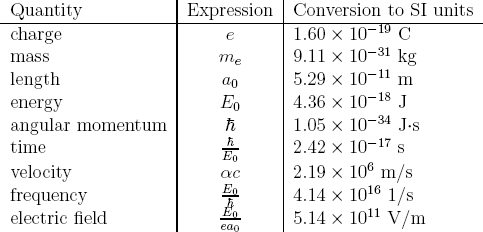
Given the chosen units for mass, charge, length, and energy, all other units can be derived from these four. Their relationship and numerical values (in SI) are summarized in Table 8.1.
We can express the TDSE in a.u. for an electron as (Exercise E8.1)
![]()
Comparing Eqs. (8.2) and (8.4), we see that the net effect in switching to atomic units is dropping all constants, equivalent to setting ħ = me = e = 1 in the equations.3 In the rest of this chapter, we will use atomic units unless otherwise noted. We also assume the particles to be electrons.
8.2 Direct simulation
We first consider a direct method for solving the TDSE (and other time-dependent PDEs alike) by converting it to a set of ODEs.4 This will enable us to start simulating quantum systems with minimum delay using standard ODE solvers.
8.2.1 Space discretized leapfrog method
We discretize space into grid points xj = jh, where h is the grid size, and j = 0, 1, …, N. The second-order differential operator ∂2/∂x2 is approximated the same way as before, Eq. (6.73a), such that
![]()
Let ψj(t) = ψ(jh, t) and Vj(t) = V (jh, t) as usual, we obtain the space discretized TDSE by substituting Eq. (8.5) into (8.4),
![]()
This is a set of N + 1 ODEs, to be solved given the initial wave function over space, ψj(0). This way, the solution to the TDSE is reduced an initial value problem.
Before we can integrate Eq. (8.6), we need to consider the fact the Schrödinger equation preserves the normalization (8.1), so an ODE solver that preserves the norm (or flux) should be used. We have discussed in Chapter 2 that the leapfrog method has this special property. It is our method of choice here.
To rearrange Eq. (8.6) suitable for leapfrog integration, we separate the wave function into its real and imaginary parts, Rj and Ij, respectively. Let
![]()
Substitution of Eq. (8.7) into (8.6) yields (Exercise E8.2)
![]()
![]()
We have assumed that the potential is real, as physical potentials are.
Besides being real, Eqs. (8.8a) and (8.8b) are in the proper form for leapfrog integration. The derivative of the real part depends only on the imaginary part, and vice versa. If we regard Rj as the general “coordinates”, and Ij as the general “velocities”, these equations mirror exactly the pair of equations (2.44) and (2.45), with Rj corresponding to rj and Ij to vj.
Let us express Eqs. (8.8a) and (8.8b) in a more compact matrix form.
Let
![]()

The matrix A is tridiagonal, so it is a band, sparse matrix.
In terms of these matrices, Eqs. (8.8a) and (8.8b) become
![]()
Note the opposite signs in front of the matrix A. This result is formally equivalent to Eqs. (2.39) and (2.40) in that the change of the “velocity” vector I depends on the “acceleration”, −AR, which is a function of “position” vector R only, like in a Hamiltonian system. In fact, the analogy goes further: Eq. (8.10) describes a general “harmonic oscillator” in the same way Eqs. (2.39) and (2.40) do a simple harmonic oscillator, recalling a(x) = −ω2x in the latter. Consequently, we can formally view RTR + ITI as a general energy, and conservation of energy in a Hamiltonian system requires that
![]()
which is a statement on the conservation of probability (8.1). We can prove this result analytically (Exercise E8.2).
Accordingly, we can formally port over the leapfrog method from Eqs. (2.41) and (2.42) to

where Δt is the step size. Equation (8.12) is the space discretized leapfrog (SDLF) method. It advances the solution one step forward, from (R0, I0) to (R1, I1), and more importantly, preserves the norm.
When the initial wave function is given at t = 0, we can march forward to obtain the wave function at later times. But, with what step size? As we saw earlier (Section 6.5.4), we also need to check the stability of an algorithm whenever finite differencing is involved in time stepping. A similar von Neumann stability analysis can be carried out for the SDLF (Exercise E8.3), and the stability criterion is
![]()
where 0 < λ < 1 is a coefficient dependent on the potential V. For free particle motion (V = 0), λ = 1. In general, the greater the potential, the smaller the λ. From experimentation, λ = ![]() should work for most cases.
should work for most cases.
Recall that for waves on a string, the stability condition (6.81) is Δt ∝ h. Why is Δt ∝ h2 in the present case? As mentioned earlier, the Schrödinger equation is first order in time, whilst the wave equation is second order in time. This accounts for the h2 dependence mathematically. Physically, the Schrödinger equation is similar to the diffusion equation. In diffusion, typified by Brownian motion such as a drop of ink in water, the particles spread out at a rate 〈x2〉 ∝ t (see Section 10.3 and Eq. (10.40)). Equation (8.13) requires that the time step must be such that a particle does not exceed the physically allowed diffusion distance.
8.2.2 Implementation
We have everything in place to start implementing the direct simulation method. We need to write a derivative function, similar to Program 4.3, appropriate to the leapfrog integrator. First we declare two arrays, R and I, to hold the real and imaginary parts of the wave function over the spatial grid. They will be initialized to the wave function at t = 0, and stepped forward according to Eqs. (8.8a) to (8.8b).
It seems straightforward enough to program this. Depending on whether dRj/dt or dIj/dt is needed, it requires only one loop to sum up the three terms in each equation. But (there is always a but, isn't there? this but is different this time), consider this: each loop needs about N operations, and since the grid size is h ~ N−1, the time step Δt required for stable integration scales as Δt ∝ h2 ~ N−2. It means to advance the solution over some time interval (say 1 unit), the number of operations scales like Nop ~ N3. Suppose N = 1000, then Nop ~ 109. This is large and taxing for an interpretive language like Python.
Thus, we need to make the above mentioned loop as efficient as possible. Fortunately, as in previous situations (see Sections 6.5.5, 6.7, or 7.2.1), the NumPy library makes it easy.5 There are two approaches. The first is to use fast matrix multiplication, realizing that A in Eq. (8.12) is tridiagonal and banded. The second is to use element-wise operations with array slicing to avoid explicit looping as in Program 6.4. We choose the second approach here for it is simpler and just as fast.
Observing from Eq. (8.8a), for instance, dRj/dt depends on Ij and its left and right neighbors, Ij−1 and Ij+1, respectively. We can thus obtain dR/dt at once by adding three arrays (up to some scaling constants) as: I, I right-shifted by one, and I left-shifted by one. This is the same method as in 1D waves discussed in Section 6.5.5 and illustrated in Figure 6.15.
The end points can be resolved assuming a given boundary condition. We will use periodic boundary conditions. Consider the actual system consisting of N + 1 grid points with ψj, j = 0, 1, …, N. Imagine identical copies of the system are placed next to each other along the x-axis. If we step past the right end point of the (actual) system, we will be at the first (left-most) point of the (virtual) system to the right. Likewise, if we go the other way and move past the left end point, we will be at the right-most point of the system to the left. We can express the periodic boundary condition as
![]()
With Eq. (8.14), the actual derivative function, sch_eqn(), is given below.
It returns dR/dt if id is zero, else dI/dt. In each case, a temporary array tmp is used to hold the first and the third terms of Eq. (8.8a) or (8.8b) before shifting, and the middle term is stored in dydt. The potential array V is built in the main program (Program 8.2). Then, the interior elements are added via slicing discussed above. Note tmp[:-2] implies all elements from the beginning up to (but not including) the second last, and tmp[2:] from the third to the end. The end points are treated separately according to the periodic boundary condition (8.14), which means that the left neighbor of the first point is the same as the last point, tmp[−1] (line 11), and the right neighbor of the last point is the same as the first point, tmp[0].
Similarly, we can use the vectorized leapfrog code (Program 2.6) which succinctly expresses the algorithm (8.12). In addition, it has the advantage of speed gain. Each of the three steps in the leapfrog method is an implicit loop, and can be computed much faster for large arrays, as is the case here. Profiling (Section S:8.B) shows that we gain about 50x speedup compared to explicit looping for N = 500.
8.2.3 Quantum harmonic motion

Figure 8.2: The probability density (top), the real and imaginary parts of the wave function (middle and bottom, respectively), in the SHO potential.
The complete code is given in Program 8.2, which yields the results below (slightly modified for plotting, Project P8.1). Figure 8.2 displays the motion of an electron in the simple harmonic oscillator (SHO) potential (2.46), ![]() . The initial wave function is a normalized Gaussian wavepacket,
. The initial wave function is a normalized Gaussian wavepacket,
![]()
The parameters x0 and σ are the center and width of the Gaussian, respectively. The variable k0 is the average momentum (at t = 0) of the wavepacket.
The results shown in Figure 8.2 are for ![]() , x0 = −3 and k0 = 0. The spatial range is set to −10 ≤ x ≤ 10, divided into N = 500 intervals (for a total of 501 grid points), so h = 0.04 and
, x0 = −3 and k0 = 0. The spatial range is set to −10 ≤ x ≤ 10, divided into N = 500 intervals (for a total of 501 grid points), so h = 0.04 and ![]() . This value of N gives us good balance between accuracy and speed. The top graph shows the probability distribution at five equidistant locations. The potential is also drawn for easy reference. The wavepacket moves to the right, accelerates and broadens as it approaches the center. Past the center, it starts to slow down and becomes narrower until the right end point where the wavepacket looks nearly identical to the original one (refocusing). Afterward, it reverses direction, and moves toward the starting position.
. This value of N gives us good balance between accuracy and speed. The top graph shows the probability distribution at five equidistant locations. The potential is also drawn for easy reference. The wavepacket moves to the right, accelerates and broadens as it approaches the center. Past the center, it starts to slow down and becomes narrower until the right end point where the wavepacket looks nearly identical to the original one (refocusing). Afterward, it reverses direction, and moves toward the starting position.
The middle and bottom graphs in Figure 8.2 show the real and imaginary parts, R and I respectively, of the wave function at three positions (left end, center, and right end). Initially, there is only the real part. With increasing t, both parts develop, and become more oscillatory toward the center. The peaks of R and the nodes of I coincide with each other (vice versa), making the probability density smooth throughout. Surprisingly, the real part does not vanish at the right end, where the imaginary part dominates. We would not have suspected this behavior based on the appearance of the probability density graph alone.
The evolution of the probability density is shown in Figure 8.3 as a function of space and time simultaneously. We can see more clearly from the surface plot the periodic motion of the wavepacket as it zigzags back and forth in time. The width of the wavepacket also oscillates periodically. We can observe in the contour plot the periodicities of both the probability density and the width more clearly. The period is close to 2π, which matches very well with the classical period of the SHO, 2π/ω from Eq. (6.11), when the mass and spring constant are unity. We can also understand these oscillations as a result of quantum revival, discussed in Section 8.5.
Based on the results so far, we should expect that the average position, i.e., the expectation value of position 〈x〉, to give a quantitative depiction of the periodic motion. Given the wave function ψ(x, t), we can calculate the expectation value for position as
![]()
For momentum p and kinetic energy T, respectively, we have
![]()

Figure 8.3: The surface and contour plots of probability density.

The last expressions in Eqs. (8.17) and (8.18) are useful for numerical calculations (see Exercise E8.5 and Project P8.2). For time-dependent systems, the above expectation values are generally a function of t.
We need to evaluate the integral (8.16) numerically. Like solving ODEs, numerical integration is a common procedure in scientific computing. We discuss several integration techniques in Section 8.A.

Figure 8.4: The expectation value of position (solid line) and the maximum of the probability density (dashed line).
Since the wave function is discretized over a regular grid, it is simplest to use Simpson's rule (Project P8.1) to evaluate Eq. (8.16). The expectation value 〈x〉 as a function of time is graphed in Figure 8.4. As expected, it indeed follows a sinusoidal pattern like the classical SHO (2.47). From visual inspection, we infer 〈x〉 ![]() −A cos t.
−A cos t.
The quantity 〈x〉 provides a bridge between classical and quantum mechanics through the Ehrenfest theorem, which describes the dynamics of physical observables governed by a set of relationships very similar to classical equations of motion. For instance, the expectation values of position and momentum satisfy (Exercise E8.4)
![]()
We see that this is just like Newton's second law with a force given by F = −〈∂V/∂x〉 (see Eq. (2.46)).
In our case, ![]() , thus F = −〈x〉. Substituting it into Eq. (8.19) yields 〈x〉 ~ −A cos t, just as observed earlier. Therefore, we can numerically confirm Eq. (8.19), m〈
, thus F = −〈x〉. Substituting it into Eq. (8.19) yields 〈x〉 ~ −A cos t, just as observed earlier. Therefore, we can numerically confirm Eq. (8.19), m〈![]() 〉 = F.6 So classical mechanics is recovered for space-averaged observables.
〉 = F.6 So classical mechanics is recovered for space-averaged observables.

Also shown in Figure 8.4 is the value of maximum probability density (right y axis) as a function of time. The maximum value, Pmax, refers to the peak of the distribution, which is approximately at the center of the wavepacket. We can think of Pmax as a measure of how quickly the wavepacket broadens since it is inversely proportional to the width (roughly). Pmax starts from the peak value at t = 0 when the Gaussian is at its narrowest. It reaches the lowest value at the moment the center of the Gaussian is at x = 0, where the wavepacket is broadest, before recovering its peak value at the right end. The cycle repeats afterwards, so the period of Pmax is half the period of the SHO. Because the SDLF method preserves the norm, the peak values of Pmax stays constant.
We can keep track of normalization continuously by computing Eq. (8.1) at regular time intervals. Figure 8.5 shows the deviation of normalization from unity, i.e., 1 − ∫ |ψ|dx. The absolute error is on the order of 10−6 given the same grid size h and step size Δt as in Figure 8.2. The absolute error is less significant than its oscillatory behavior: it shows that the error is bounded, much like what we saw for the energy of the SHO using the leapfrog method (Figure 2.7). Here we see again that the leapfrog method, being finite order and symplectic, exactly preserves a numerically inexact result. Overall, the SDLF is a direct, robust method for solving the TDSE.
It is interesting to observe the absolute error exhibiting a period equal to half of the SHO's period, just like Pmax. Correlating with Figure 8.4, we see that the error is largest when the wavepacket is at the end points when it is narrowest. A sharper wave function requires a denser grid to maintain accuracy. Making h or Δt smaller can help reduce the magnitude of the error. A more effective method is to make our numerical scheme unitary (norm preserving) to begin with, an approach we take next.
8.3 Free fall, the quantum way
The SDLF is an explicit method that marches forward given the initial wave function. It is direct and robust, provided that the stability condition (8.13) is fulfilled, which is also its major limitation. In this section, we discuss a first order split-operator method, simply referred to as the split-operator method below, which removes this limitation. The method is particularly useful for motion in open space such as scattering problems or unidirectional motion like free fall. We apply it to simulate the free fall of a quantum particle.
8.3.1 The split-operator method
To develop the split-operator method, we rewrite Eq. (8.4) more concisely utilizing the Hamiltonian H,
![]()
where we assume for the moment that the potential is time-independent.
Formally, we can write the solution to Eq. (8.20) as [80]
![]()
It is understood that the function of an operator ![]() is defined through its Taylor series
is defined through its Taylor series
![]()
If the effect of ![]() is small, we can retain the first few terms for accurate representation of the operator function.
is small, we can retain the first few terms for accurate representation of the operator function.
The operator e−iH(t−t0) is called the evolution operator for it advances the wave function from t0 to t. The evolution operator is unitary, that is, it preserves the normalization at all time, ∫|ψ(x, t)|2 dx = ∫|ψ(x, t0)|2 dx (see Exercise E8.6). Since its exact solution is unknown, we must approximate it.
Let Δt = t − t0, ψ0 = ψ(x, t0), and ψ1 = ψ(x, t0 + Δt). We have from Eq. (8.21)
![]()
Assuming Δt is small, we expand e−iHΔt according to Eq. (8.22), and to first order we have
![]()
This is Euler's method for the TDSE. But, this form turns out to be numerically unusable, because it is nonunitary and unstable no matter how small Δt is (Exercise E8.3).
The split-operator method, also known as the Crank-Nicolson method originally applied to heat conduction problems [21], takes a symmetric approach by splitting the exponential operator in halves, and applying the first-order truncation to each half as

It can be shown that this result is accurate to first order in Δt and agrees with the Euler method (8.24) (Exercise E8.6). However, though an approximation, Eq. (8.25) is unitary,

Physically, it means that the split operator preserves the normalization of the wave function regardless of the size of Δt.
Substituting Eq. (8.25) into (8.23) and acting on both sides by the operator in the denominator, we obtain
![]()
To look at this relationship another way, we have
![]()
If we were to replace ψ1 on the RHS by ψ0, we would recover Euler's method (8.24). The effect of the split-operator method is to replace ψ0 in Euler's method by the average (ψ1+ψ0)/2. This little trick makes a big difference.
To construct a numerical scheme, we discretize the Hamiltonian operator in Eq. (8.27) the same way as in SDLF over the spatial grid xj = jh. Let ![]() . After some algebra (Exercise E8.7), the final result is
. After some algebra (Exercise E8.7), the final result is

Unlike the explicit SDLF method (8.12), the split-operator method is an implicit method: the value ![]() depends not only on previous values
depends not only on previous values ![]() at t0, but on the current values
at t0, but on the current values ![]() at t as well. Rather than simply marching forward, we have to invert Eq. (8.29) for all values of
at t as well. Rather than simply marching forward, we have to invert Eq. (8.29) for all values of ![]() simultaneously at each step. This is the price we pay, in exchange for absolute stability guaranteed in Eq. (8.29) (Exercise E8.8).
simultaneously at each step. This is the price we pay, in exchange for absolute stability guaranteed in Eq. (8.29) (Exercise E8.8).
Equation (8.29) had first been solved using clever recursion techniques [37]. We use a much simpler matrix method. Let us assume that, for the time interval of interest, the wave function at the boundaries are so small as to be negligible, ψ0 = ψN = 0 (fixed ends). This can be interpreted in two ways. One is that the spatial range is so large that the particle (wavepacket) is far away from either end of the box. The other is that the boundaries are hard walls (infinite potentials) so the particle does not penetrate them. We will revisit this point shortly in discussing the results (Section 8.3.2).
Let
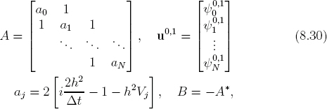
and assuming fixed-end boundary conditions, we can express Eq. (8.29) in matrix form as
![]()
Equation (8.31) is the final result of the split-operator (Crank-Nicolson) method in matrix formulation. Given the wave function u0 at t0, we obtain the new wave function u1 at t + Δt by solving a linear system of equations. Because we must do this at each step, it would be very costly in general. However, we are helped by two facts: the matrix A is a tridiagonal, band matrix, and it is time-independent (if V = V (x)). The tridiagonal nature of A is due to approximating ∂2/∂x2 by a three-point scheme (8.5).
We can use special matrix solvers designed for band matrices in the SciPy library, which reduce the number of operations linearly in N rather than N2 in general. To use band matrix solvers, we first need to express the matrix A in the required format.

Figure 8.6 illustrates an example of representing a tridiagonal matrix as a band matrix. Our original matrix (A, source) has a maximum of three nonzero elements in each column. The band representation (B, target) is chosen to be a matrix with three rows and the same number of columns. The resultant matrix is just the band of the original matrix being flattened. The first and the last elements of the target, B11 and B35 respectively (•), are dummy fillers not used in actual computation, so they can be set arbitrarily. For general band matrices, we just need to increase the number of rows to represent it properly. If u is the number of elements above the diagonal, then Aij = Bi−j+u+1,j, i ≤ j. For instance, we have u = 1 for the tridiagonal matrix, such that A34 = B14 = 1, and A44 = B24 = 4, etc.
The actual implementation of the split-operator method is straightforward. It consists of six lines shown below, taken from the full Program 8.3.
  1A = np.ones((3, N+1), dtype=complex)             # prepare band matrix A, B
A[1,:] = 2*(2j*h*h/dt − 1 − h*h*V)
  3dB = − np.conjugate(A[1,:])                               # diagonal of B
 ......
  5      C = dB*psi                                                     # prepare RHS Eq. (8.31)
      C[1:−1] −= (psi[:−2] + psi [2:])
  7       psi = solve_banded((1,1), A, C)                    # band matrix solver
The first line creates a 3 × (N + 1) matrix, data-typed complex and filled with ones initially. The second line replaces the second row with the complex diagonal elements from Eq. (8.30) using vector operation, completing the band representation of matrix A. The third line creates a 1D array containing the diagonal of matrix B in Eq. (8.30) only, which is the negative complex conjugate of the diagonal of A.
Next, we prepare the RHS of Eq. (8.31). Rather than direct matrix multiplication, we obtain it from the RHS of Eq. (8.29) because SciPy does not yet have a banded matrix multiplication routine. Line 5 computes the first term on the RHS of Eq. (8.29), i.e., the diagonal elements of Bu0 in Eq. (8.31). This is why we did not need the full matrix B above. The next line subtracts the last two terms, the left and right neighbors, respectively, using the same shift-slicing technique as before (Section 8.2.2). For fixed ends, we neglect the boundary points, since ![]() . Now, we have completed the RHS of Eq. (8.31).
. Now, we have completed the RHS of Eq. (8.31).
The last line (line 7) calls the SciPy band matrix solver, solve_banded(), to obtain the solution ψ1 at t + Δt. The function requires a minimum of three parameters as
solve_banded((l,u), A, b)
It solves a linear system, Ax = b, assuming A is in band matrix format. The (l,u) pair specifies the lower and upper diagonals, i.e., the numbers of elements below and above the diagonal in the band, respectively, such that the band width is l+u+1. For our tridiagonal matrix, we have (l,u)=(1,1) in line 7.
8.3.2 Quantum free fall
As a test case, we apply the split-operator method to the free fall of a quantum particle. We choose the linear potential to be
![]()
The parameter a plays the same role as the gravitational acceleration in free fall, mgy. Such a scenario exists for electrons in a constant electric field.

Figure 8.7 shows the results from Program 8.3. The initial wave function is again a Gaussian (8.15), and the acceleration is a = 2. The center of the wavepacket falls toward the negative x direction as expected. It also broadens as before, but unlike the SHO potential, there is no refocusing effect in the linear potential, and the wavepacket just keeps broadening.
Since a wavepacket is made up of different momentum components which spread out at different speeds, the broadening is irreversible if there is no refocusing force to restore the motion. The SHO potential provided a restoring force causing the wavepacket to narrow and broaden periodically (Section 8.2.3). The linear potential, however, yields a constant force that accelerates different parts of the wavepacket equally, and the spreading continues unabated.
Another difference between the linear and SHO potentials is that free fall motion is unidirectional and has no lower bound. As a result, when waves inevitably reach the finite boundaries in our simulation, it will be reflected due to our assumption that the boundary values are small, ψ0 = ψN ![]() 0. We have seen similar reflections on a vibrating string (Section 6.5.5). This causes the leading edge of the waves to interfere with its self reflection. The growing ripples we see in the last three frames (Figure 8.7) are self-interference patterns. These patterns are clearly an artifact of our domain being finite, and not real physical effects. In infinite space, the wavepacket would just keep spreading, so the amplitude would become ever smaller while its width ever larger. This cautions us that, in interpreting simulation results or comparing with observations such as experimental data, we should consider boundary effects carefully, and take steps to minimize them if possible. Conversely, as stated earlier, we can interpret the results as free fall between hard walls, in which case the interference patterns are real and due to actual reflections.
0. We have seen similar reflections on a vibrating string (Section 6.5.5). This causes the leading edge of the waves to interfere with its self reflection. The growing ripples we see in the last three frames (Figure 8.7) are self-interference patterns. These patterns are clearly an artifact of our domain being finite, and not real physical effects. In infinite space, the wavepacket would just keep spreading, so the amplitude would become ever smaller while its width ever larger. This cautions us that, in interpreting simulation results or comparing with observations such as experimental data, we should consider boundary effects carefully, and take steps to minimize them if possible. Conversely, as stated earlier, we can interpret the results as free fall between hard walls, in which case the interference patterns are real and due to actual reflections.
We note that the split-operator method as implemented initially preserves the normalization (8.1) to a high degree of accuracy. As time increases, error starts to grow due to waves reaching the boundaries. The leading waves have higher momentum so they are highly oscillatory as seen in Figure 8.7. To maintain accuracy, smaller grids are needed (see Project S:P8.1). A more accurate, second-order split evolution operator (SEO) method is developed in Section S:8.1.
Figure 8.8 shows a contour plot of the probability density as a function of time using the same parameters as in Figure 8.7. In addition to broadening and self-interference discussed above, we see the center of the wavepacket following a parabolic curve (before reaching the boundary). The classical free fall motion is given by Eq. (2.2), which in our case is x = 5−t2 (a = 2). This is drawn as the dashed line in Figure 8.8. We see good agreement and an interesting connection between quantum waves and classical trajectory motion, which is a another clear demonstration of the Ehrenfest theorem (8.19). A quantum wave moves along the classical path of a particle in terms of average position and force (expectation values).

Figure 8.8: The probability density of a quantum particle in free fall. The dashed line shows the classical path.
8.3.3 Momentum space representation
From the motion of the wavepacket in coordinate space above, we have learned a good deal about the momentum (velocity) of the particle. Better yet, quantum mechanics allows us to get an entirely different, but equivalent, view from the wave function in momentum space. In a.u., the momentum is equal to the wavevector ħk = k.
The wave function in momentum space, ϕ(k, t), and in coordinate space, ψ(x, t), are related by a pair of reciprocal Fourier transforms (5.34) and (5.35),
![]()
![]()
It is sometimes convenient to use a shorthand notation for these Fourier transforms, ![]() , and
, and ![]() (we have omitted t in the shorthand to denote the actual variables x and k).
(we have omitted t in the shorthand to denote the actual variables x and k).
Just like |ψ|2 giving the probability in position space, |ϕ(k)|2 gives the probability of finding the particle with momentum k. And ϕ(k) is normalized if ψ(x) is as well, i.e., ∫|ϕ(k, t)|2dk = ∫|ψ(x, t)|2dx = 1.
Since our wave function ψ(x, t) is discrete over the space grid, it is efficient and straightforward to evaluate Eq. (8.33a) with the FFT method (if you have not done so already, now would be a good time to review Section S:5.B).
Suppose we sample M points at equal intervals δx = h over the spatial range (i.e., period) d = Mh. From Eqs. (S:5.18) and (S:5.20), and according to Section S:5.B.3, the momentum grid points are determined by
![]()
where δk = 2π/d is the interval in momentum. The range of momentum is q = Mδk = 2π/h, again in accordance with Eq. (S:5.21). Like δk, the spatial interval is related to q reciprocally by δx = 2π/q. To use FFT, we make the number of grid points M a power of 2, i.e., M = 2L, L = integer. By our convention (Program 8.3), if N is the number of intervals, then N = M − 1.
In Eq. (8.34), we are interpreting the Fourier components as made up of positive and negative momentum values. Because the transform has a period M, we have ϕ(kj) = ϕ(kj+M). Even though all momentum values can be treated as being positive mathematically, we require half of them to be negative from physical point of view. The FFT storage scheme for the components is outlined in Table S:5.1.
The momentum distribution is presented as a profile on the k-axis in Figure 8.9 and as a density contour plot in Figure 8.10 in terms of k and t (Project P8.4). The results are obtained from a slight modification of Program 8.3 where line 37 is replaced by the following,
phi = np.array(fft. fft_rec (psi, L))                           # FFT
phi = np.concatenate((phi[M//2:], phi[:M//2]))       # re−order neg to pos k
pb = phi.real**2 + phi.imag**2
The parameter L is equal to 10, so M = 1024 and N = 1023. After taking the FFT using the recursive function fft_rec() from our library, the array phi[] contains the resultant momentum wave function. The second line pulls the second half of the array in front of the first half so it is in the order of increasing k per Eq. (8.34) after concatenation (see Eqs. (S:5.41) and (S:5.42)).

Initially the momentum profile is a Gaussian (in k space), since the Fourier transform of a Gaussian is another Gaussian. Furthermore, the widths in coordinate and momentum spaces are related by the uncertainty principle (do not confuse Δx and Δk with sampling intervals δx and δk)
![]()
In the present case, we had Δx ~ 2σ = 1, so Δk should be on the order of one. This may be assessed from Figure 8.10. If we increase σ, Δk will decrease proportionally, and vice versa.
Both figures show that, at the beginning, the profile keeps its initial shape with no apparent broadening, in stark contrast to position space where broadening happens rather quickly. Imagine the wavepacket was in free space. Since there would be no force, the momentum as well as the kinetic energy of the particle must be conserved, and we would expect no spreading at all.
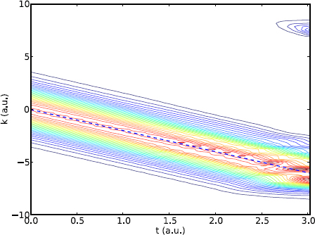
Figure 8.10: The momentum density of a quantum particle in free fall. The dashed line shows the classical relation v = v0 − at (a = 2).
In free fall, there is a constant acceleration in the negative direction. As a result, we see the entire momentum profile moving in that direction, following the classical linear relation, v = v0 − at (Figure 8.10), just like its classical path (Figure 8.8). As time increases, the leading edge reaches the boundary, equivalent to hitting a hard wall. Part of the wave is being reflected and self-interference occurs as discussed earlier. The momentum distribution begins to deform from a perfect Gaussian, and smaller structures develop on top of the Gaussian. Toward the end at t ~ 3, we see a spike at a positive momentum k ~ 7. In large part the spike is due to the acceleration of the center-left portion of the wavepacket reaching that speed, and being reflected by the wall.
The center of the momentum is zero initially, but since Δk ~ 1, there is a significant portion of the distribution near k ~ ±1. Classically, the leading edge (k = v0 ~ −1) at t ~ 3 would have a displacement of ![]() (Figure 8.8), and a velocity of v = v0 − at ~ −7. Its position, assuming an initial position x0 = 5 and a spread of ±1, would be roughly x ~ −7 to −9, just reaching the wall located at −10. Upon colliding with the wall, the velocity would be reversed, giving rise to the spike at k = −v ~ 7.
(Figure 8.8), and a velocity of v = v0 − at ~ −7. Its position, assuming an initial position x0 = 5 and a spread of ±1, would be roughly x ~ −7 to −9, just reaching the wall located at −10. Upon colliding with the wall, the velocity would be reversed, giving rise to the spike at k = −v ~ 7.
As seen earlier, this effect is due to our domain being finite. If we interpret the physical boundaries as actual hard walls, the particle would bounce up and down, with self-interference making it look less and less like a localized classical particle with time. Interestingly, if we evolve the system long enough until the so-called revival time (8.55), nearly all the distribution will be contained in the spike, and the cycle repeats.
8.4 Two-state systems and Rabi flopping
In the last two sections we discussed quantum motion under time-independent potentials. There are situations where a quantum system is subject to a time-dependent potential, causing it to change states, a process called quantum transition. For instance, if a hydrogen atom is exposed to an oscillating laser field, the electron can jump to an excited state. When a system interacts with an external field, it is an open system.
We are interested in quantum transitions in this section. For simplicity and clarity, we will consider only two-state systems here, and will keep the model brief. A full, unlimited model with a worked example is developed in Section S:8.2, which should be reviewed for more details.
8.4.1 Two-state model for transition
Let H0 be the unperturbed Hamiltonian of the system in the absence of the laser field, and u1 and u2 be its two states, called eigenstates (like eigenmodes in Chapter 6; see Chapter 9 for eigenstate problems). The solutions of the unperturbed system satisfy
![]()
where E1 and E2 are the eigenenergies of states 1 and 2, respectively. We assume u1, u2 and E1, E2 are known, e.g., they may be the up or down states of a spin, or the lowest two states of a particle in a box (S:8.39). The eigenstates are also orthonormal, i.e., (integration limits omitted)
![]()
We prepare the system so that the particle is in state 1 at t = 0, and then turn on the laser. The particle will respond to the laser force, and start mixing with state 2. We expect the wave function of the particle at t, ψ(x, t), to be a superposition of the two states as
![]()
where a1(t) and a2(t) are the expansion coefficients (generally complex). Note that we have included the exponential time factors of stationary states in Eq. (8.38).
The interpretation of the coefficients is that the probabilities of finding the particle in states 1 or 2 are given by |a1(t)|2 and |a2(t)|2, respectively. They are also called occupation (or transition) probabilities. Because the total probability is conserved, we have
![]()
To solve for a1(t) and a2(t), we substitute ψ(x, t) of Eq. (8.38) into the Schrödinger equation iħ∂ψ/∂t = (H0 + V (x, t))ψ, where V (x, t) represents the interaction with the laser field (see Eq. (S:8.40)). After some algebra and using Eq. (8.36) for cancellations (see Section S:8.2), we obtain
![]()
The notation ![]() 1,2 represents derivative with respect to time.
1,2 represents derivative with respect to time.
Equation (8.40) is valid for all space and time. To extract the coefficients, we project it to the eigenstates u1 and u2. For instance, we can multiply both sides of Eq. (8.40) by ![]() , and integrate over x. Using the orthogonality relation (8.37), the
, and integrate over x. Using the orthogonality relation (8.37), the ![]() 2 term drops out. The same can be done with
2 term drops out. The same can be done with ![]() . The final result after projection is
. The final result after projection is

where ω = (E2−E1)/ħ is the transition frequency, and the matrix elements Vmn are defined as
![]()
Equation (8.41) is the central result of the two-state model (a subset of Eq. (S:8.33)). It can be integrated if the laser field V (x, t) is given.
8.4.2 Rabi flopping

Figure 8.11: State population for a laser duration τ = 600. The dotted line shows a shifted Rabi flopping function cos2(ΩRt + φ), Eq. (8.49a).
As an example, we carry out a calculation for a particle in the box (infinite potential well) with Program S:8.1 which integrates Eq. (8.41) with the RK4 method. The ground and the first excited states are included (N = 2), and the laser field interaction is given by Eqs. (S:8.40) and (S:8.41). The laser has a center frequency equal to the transition frequency between the two states, and a pulse duration of τ = 600 a.u. The rest of the parameters are kept the same as in Figure S:8.8. The results are shown in Figure 8.11.
The system starts out in state 1, its population P1 decreases continuously to very nearly zero. At the same time, the population P2 of state 2 increases in such a way that the net loss in P1 becomes the net gain in P2. The two states oscillate back and forth between practically 0 and 1. This behavior may be understood in a simplified picture known as Rabi flopping.
Rabi flopping is an important phenomenon in externally driven two-state systems. To avoid unnecessary clutter, we assume a monochromatic laser field tuned to (resonant with) the transition frequency,
![]()
This form of the field will help us see more clearly the core idea of Rabi flopping. In numerical calculations such as Figure 8.11 we still use realistically enveloped pulses like Eq. (S:8.41).
For the particle in a box, the transition matrix elements can be written explicitly from Eq. (S:8.44) as
![]()
where V0 = −16eaF0/9π2 (e is electron charge, a box width, F0 field amplitude). The diagonal matrix elements being zero (or close to zero) is a common property in dipole transitions of many systems.
Substituting Eq. (8.44) into (8.41) gives us

Equation (8.45) is analytically solvable, but the solutions may be simplified with a useful approximation. Over a time period long compared to 1/ωL, the factors exp(±2iωLt) in Eq. (8.45) will undergo many oscillations. Their net average values will be close to zero, i.e., 〈exp(±2iωt)〉 ![]() 0. We can then drop them from Eq. (8.45). This is called the “rotating wave approximation” (RWA) [64]. Within RWA, we arrive at two simplified equations
0. We can then drop them from Eq. (8.45). This is called the “rotating wave approximation” (RWA) [64]. Within RWA, we arrive at two simplified equations
![]()
Differentiating both sides of Eq. (8.46), we obtain the following equivalent second-order differential equations,
![]()
The quantity ΩR is the Rabi frequency. It depends on the interaction strength only, not on the laser frequency.
Equation (8.47) is a pair of well-known SHO equations whose solutions, subject to the initial condition a1(0) = 1 and a2(0) = 0, are
![]()
The occupation probabilities of the two states at time t are
![]()
![]()
Clearly, P1(t) + P2(t) = 1, as required by Eq. (8.39). The two states flip-flop back and forth with the Rabi frequency ΩR. This is Rabi flopping [74]. The frequency can be controlled through the laser field strength V0. Rabi flopping occurs in many situations, such as nuclear magnetic resonance, quantum computing and optics. It is one of the most important ideas in quantum optics.
Going back to Figure 8.11, we can understand the oscillations between 0 and 1 as a result of Rabi flopping. Recall that the results are for a realistic pulse, Rabi flopping will be significant only after the pulse has ramped up. In a complete Rabi cycle the two states are populated and depopulated completely and complementarily. We have superimposed P1(t) from Eq. (8.49a) in Figure 8.11 (dotted line) to simulate the oscillation for an idealized, infinitely long, monochromatic laser. It is phase shifted to account for the ramping up stage. We can see that during the middle part of the laser there is good agreement between numerical results and the ideal solutions.
Although no simple analytic solutions for Rabi flopping are known with an enveloped laser pulse described by Eq. (S:8.41), our numerical simulations are straightforward and the results demonstrate the universal nature of the important phenomenon (see Project S:P8.9 for Rabi flopping in hydrogen atoms). The oscillation frequency is dependent on the laser strength, and independent of laser frequency. The longer or stronger the pulse, the more cycles of Rabi oscillations. The laser frequency is responsible for the small variations (step structures) as discussed in Section S:8.2.2.
8.4.3 Superposition and the measurement problem
In Rabi flopping (8.48), we have a system whose wave function ψ is a superposition of two states ϕ1 and ϕ2,
![]()
where ϕ1,2 = u1,2 exp(−iE1,2t/ħ) (see Eq. (8.38)). At any given time, the wave function is a coherent sum of the two states, i.e., both states exist simultaneously within ψ. The probabilities of finding the states are cos2(ΩRt) and sin2(ΩRt), respectively. Quantum mechanics prescribes exactly, and deterministically, how the probabilities change with time.
How do we realize the probabilities? Measurement, of course. When we make a measurement, we will find the system in either state 1 or 2, not both. But quantum mechanics never tells us which state we will get, only the probabilities. The system would evolve just fine without any measurement. A measurement seems to force the system to reveal itself. How does it happen? What state was the system in just before we made the measurement? If we regard the two states as a cat being dead or alive, we have the well-known Schrödinger's cat problem.
Because the action of measurement is not modeled in quantum mechanics, the answers to the above questions are unknowable within the confines of quantum mechanics. Essentially, this is the measurement problem, and is open to interpretation. A commonly accepted view is the Copenhagen interpretation which holds that the system ceases to be a coherent superposition of states and collapses to one state or the other when a measurement is made. To put it another way, measurement destroys the system. Even though this does not quite answer how the system stops being a superposition of states, it is an answer. In fact, this is one of the intriguing aspects of quantum mechanics, and searching for an answer can get quite philosophical, and metaphysical sometimes. Fortunately, it does not hinder our ability to do quantum mechanics, and least of all, to simulate quantum systems.
8.5 Quantum waves in 2D
As seen from above, we can create a superposition of states, or a coherent state, with external perturbations like laser excitation. After the external interaction is turned off, the coherent state will continue to evolve but with different characteristics than single stationary states. The numerical methods we discussed above also enable us to study coherent states in higher dimensions. Below we will explore an example in 2D and examine the evolution in both coordinate and momentum spaces.
Let us consider a coherent state prepared at t = 0 in a 2D box (infinite potential well) as


This is a normalized compact wave function that is nonzero only within a rectangular region σx × σy centered at (x0, y0).
The state will evolve similarly to the expansion (8.38), which in 2D reads
![]()
The basis functions um and un are the same as Eq. (S:8.39), and the eigenenergies are Emn = Em + En, the sum of individual eigenenergies Em and En from Eq. (S:8.39). We can determine the amplitudes amn from the wave function at t = 0 as (see Exercise E8.9)

A time sequence of probability densities |ψ|2 is shown in Figure 8.12. The calculations are done with Program 8.4. We choose a square well of size a = 10, and a symmetric coherent state with σx = σy = 2 placed at the center of the well. This is a relatively narrow wavepacket, and to adequately represent the state, we include N = 20 basis states in the expansion in each dimension, so the total number of states is N2 = 400.
Initially the wavepacket broadens as expected (Figure 8.12, top row). Starting t = 1.4, we see interference effects on the outer edges of the distribution from reflected waves from the wall. Increasingly intricate interference patterns are developed at later times (t = 2 and 3), showing the level of complexity a quantum wave is capable of exhibiting. You should play with Program 8.4, e.g., setting the initial wavepacket off center, looking at the imaginary part, etc. We had seen 2D classical waves on a membrane (Section 6.7) also showing similarly interesting interference patterns (Figures 6.18 and 6.19). But quantum waves can display more entangled wave pockets (Figure 8.12, middle row) at a comparable level of energy, because the time-dependent wave functions are complex.
As time increases further, the number of pockets decreases and the wave function starts to reassemble itself into the original state at t = tR ~ 63.7. Thereafter, it repeats as if time had been reset periodically at tR, e.g., ψ(t = 0.5) = ψ(t = 64.2), etc. This phenomenon is known as quantum revival, and tR the revival time (see below).
The corresponding momentum probability density |ϕ(kx, ky, t)|2 is shown in Figure 8.13. To obtain the momentum wave function, we calculate the 2D FFT of ψ(x, y, t) by inserting the following line in Program 8.4
phi = np.fft. fft2 (wf)
The results show that the momentum distribution changes little in the beginning, t = 0 and 0.5. When the leading edge of the wave comes in contact with the wall, the momentum distribution begins to change substantially due to the “external” forces from the wall. The large momentum components on the perimeter (t =1.4 to 40) are significantly well separated from the initial distribution. All these are in accord with the 1D case (Figure 8.9).
What is new, however, is the clear reciprocal relationship between the position and momentum spaces depicted in Figures 8.12 and 8.13. They are essentially optical diffraction or interference patterns of each other [8]. For instance, we can think of the initial wave function at t = 0 in position space as a single aperture. The diffraction pattern through a single aperture would correspond to the momentum distribution. The smaller the aperture, the wider the diffraction spot. At t = 40, we can think of the four peaks as small “holes” spaced-out in position space (Figure 8.12, bottom left). The resulting interference pattern in momentum space has rows of small dots stacked over each other, forming a larger square. The size of the square is related to the size of the holes in position space, and the size of the dots to the spacing between the holes. For example, if the size of the holes is reduced, the square would grow; and if the spacing between the holes is reduced, the dots would get bigger. Conversely, we can run the argument backward from momentum space to position space, and arrive at similar conclusions.
Of course, interference of waves can be mathematically represented as Fourier transforms. Evolution of 2D quantum waves in Figures 8.12 and 8.13 graphically describes these relationships very clearly. As in position space, we observe quantum revival in the momentum distribution in the last two frames in Figure 8.13 (t = 63.7 and 64.2).
In the above example, the initial interference occurs primarily between the expanding wave and the reflected wave off the walls. We look in the next example at intrawave interference. We construct the initial state by a superposition of two wavepackets that have the same form as Eq. (8.51) but centered at different locations (Project P8.6). Shown in Figure 8.14 are two localized wavepackets initially placed at (4, 4) and (6, 6), respectively. The corresponding momentum density is given in Figure 8.15.
In position space, the waves merge and intrawave interference is significant up to t = 1. Because no external forces are involved at this stage, the momentum distribution remains substantially the same and little visible changes are seen between t = 0 and 1. Starting from t = 1.3, collision and reflection from the walls cause the wave function in both spaces to form highly entangled pockets, as was seen earlier.

Figure 8.14: Probability density in 2D well of two localized wavepackets.
Note that in the beginning, the wave function in position space is along the upper-left to lower-right diagonal, but in momentum space the distribution is in bands oriented from the lower-left to upper-right direction, such that the two distributions are approximately perpendicular to each other. The reason can be understood in analogy to optical diffraction alluded to earlier. The lengths and widths of the bands, as well as the fine structures within each band, are related to the size and separation of wavepackets in position space.
Quantum revival
A coherent state of an isolated, finite quantum system has an interesting property: periodic revival of its wave function. We have seen an example of this from Figures 8.12 and 8.13. Let us consider a coherent state expanded in the basis functions for a particle in a box (S:8.39)

Figure 8.15: Momentum density corresponding to Figure 8.14.
![]()
where E1 = π2ħ2/2mea2 is the ground state energy.
We see that the exponential factors are periodic if E1t/ħ = 2πj, j = 1, 2, 3, etc. Taking the smallest multiple, we define the revival time as
![]()
The wave function is periodic in tR, ψ(t + tR) = ψ(t). For an electron in a box with width a = 10, the period is tR = 127.3 a.u.
The period observed from the 2D box (Figure 8.12) is half this value, 63.7. The ground state energy in 2D is twice that in 1D, so the revival time is halved according to Eq. (8.55).
Classically, a particle with energy E (or ![]() ) in a box would bounce from wall to wall periodically at
) in a box would bounce from wall to wall periodically at
![]()
This classical result depends on the energy, as we intuitively expect. However, the quantal result (8.55) does not show any dependence on the energy of the coherent state at all. It is determined solely by the system parameters. The two results seem inconsistent. Worse, they also seem incompatible with the Bohr-Sommerfeld correspondence principle which states that the behavior of a quantal system should approach its classical description in the limit of large quantum numbers (semiclassical limit).
This suggests a deeper connection than the wave function alone. Though the wave function revives periodically, physical observables do not necessarily vary with the same revival period. In fact, we have seen hints to a possible resolution of this incompatibility problem in the connection between the expectation value of position and the classical motion in the SHO (Figure 8.4).
To be concrete, let us assume only two states are included,
![]()
The expectation value of position is given by
![]()
We see that 〈x〉 oscillates with a period 2πħ/ |Em − En|, which is different than the revival period (8.55). What is more, the energies of the states enter the equation. It shows that the oscillation period is inversely proportional to the difference of eigenenergies, not the eigenenergies themselves.7
Let us take the semiclassical limit, m, n ![]() 1 but keep m = n + 1, the oscillation period reduces to
1 but keep m = n + 1, the oscillation period reduces to
![]()
where we have used En = n2π2ħ2/2mea2. This semiclassical result agrees with the classical prediction, Eq. (8.56). In this way, we have resolved the apparent incompatibility in the correspondence principle. This oscillation period tsc, rather than the revival time tR, should be compared between classical and quantal predictions.
In general, we can construct a coherent state in the semiclassical limit by including a number of eigenstates clustered around n0 ![]() 1 [87]. Then, Eq. (8.59) can be generalized to
1 [87]. Then, Eq. (8.59) can be generalized to

The period tsc can be much smaller than tR. We leave further exploration of quantum revival to Project P8.7.
Chapter summary
We studied numerical simulations of time-dependent quantum systems including dynamic evolution of closed systems and quantum transitions in open systems. We presented several efficient and easy-to-use methods appropriate for solving the TDSE, breaking down the traditional unsolvability barrier in quantum mechanics where very few meaningful time-dependent problems are analytically solvable. This enabled us to learn by doing quantum mechanics rather than by just studying it.
The easiest way to get started is the explicit SDLF method, Program 8.2. This method converts the TDSE into a familiar system of ODEs, and we only need to change the initialization for different energies, potentials, etc. It is norm preserving and robust, provided the time step satisfies the stability criterion. The drawback is that this limits its speed for very accurate calculations. It is the recommended method because it is simple to understand and program, easy to implement boundary conditions, and requires only knowledge of ODE solvers.
Alternatively, we can use the first order split-operator method (Crank-Nicolson) which is fast and stable. But it is implicit and requires a banded matrix solver for speed. It is suitable for short-time evolution or weak potentials.
We discussed quantum transitions in external fields within a two-state model. We can obtain state occupation probabilities directly, which oscillate between the two states in a superposition. We also studied coherent states in position and momentum spaces, including quantum revival. In addition, we discussed general numerical integration techniques and banded matrix handling.
8.6 Exercises and Projects
Exercises
| E8.1 | (a) Check the atomic unit system in Table 8.1, evaluate the numerical values for the fine structure constant α, the Bohr radius a0, and the Hartree E0, in Eq. (8.3). Also, prove the identity
For electrons, m′ = 1, and the above equation reduces to Eq. (8.4). |
| E8.2 | (a) Fill in the steps from Eq. (8.6) to Eqs. (8.8a) and (8.8b). (b) Prove Eq. (8.11) by explicit differentiation. |
| E8.3 | Analyze the stability condition of the space discretized TDSE. Assume the potential is zero in this exercise.
(a) Apply Euler's method to Eq. (8.6), and carry out a von Neumann stability analysis. Show that there is no stable step size in general. (b) Repeat the above with the leapfrog method to find the stability criterion for the SDLF. |
| E8.4 | The dynamical evolution of an observable O is given by the Ehrenfest theorem [44]
where [O,H] is the commutator between the operator O and the Hamiltonian H. Using Eq. (8.62), verify Eqs. (8.17) and (8.19). |
| E8.5 | Decompose the wave function into real and imaginary parts as ψ(x, t) = R(x, t) + iI(x, t). Show that:
(a) the expectation value of momentum from Eq. (8.17) is
(b) the expectation value of kinetic energy (8.18) is similarly
(c) the probability current defined as
The results show that if the wave function is purely real or imaginary aside from an overall multiplication constant, then 〈p〉 = 0 and J = 0. Stationary states are in this category. For nontrivial time-dependent processes we are dealing with in this chapter, they are nonzero. |
| E8.6 | (a) Let U = e−iH(t−t0) be the evolution operator. Show that U is unitary, i.e., the product with its adjoint is unity, U†U = 1.
Given U and Eq. (8.21), show that ∫ |ψ(x, t)|2 dx = ∫ |ψ(x, t0)|2 dx. (b) Expand the denominator in Eq. (8.25) in a Taylor series, and show that the split operator agrees with e−iHΔt to first order. |
| E8.7 | Using Eq. (8.5), discretize the split operators in Eq. (8.27) to prove Eq. (8.29). |
| E8.8 | Conduct a von Neumann stability analysis of the split-operator result (8.29). Show that it is stable regardless of the time step. |
| E8.9 | Given the initial wave function (8.51), prove the expansion coefficients (8.53). |

Projects
| P8.1 | Explore the evolution of a wavepacket in the SHO potential, and use Program 8.2 as the base program. In this and other projects below, assume the wavepacket describes an electron.
(a) Generate the spatial and temporal probability density shown in Figure 8.3. To prepare data, declare two empty lists before the main loop, say ta and Z. Inside the loop, periodically append the probability density array (over the spatial grid) to Z and time to ta. This is one slice of the probability density at a given time. The above procedure should be the same as in Program 8.3. Terminate the loop after certain amount of time, e.g., t = 8. Adjust the frequency of sampling so that roughly 50 slices of data are recorded. After exiting the loop, the data Z is a list of arrays, i.e., a two-dimensional array. Prepare the space-time grid using X, Y = np.meshgrid(x, ta) where x is the spatial grid. Make a surface plot as usual (see Programs 8.3 or 7.2, for example). You can exclude the end regions |x| With the same data, reproduce the contour plot in Figure 8.3. Also try plt.imshow() to change the appearance of the contour plot to an image (see Program 8.4). (b) Calculate and graph the expectation value of position 〈x〉 as a function of time. Let pb be the probability density array at t. An easy way to approximate 〈x〉 is to convert the integral (8.16) into a sum with the NumPy sum() function, xexp = h*np.sum(x*pb) Here, h is the grid size. The expression np.sum(x*pb) is equivalent to ∑ xi|ψi|2. Note that xexp is a number (scalar). Put this line inside the main loop, append xexp to a list, and plot it at the end. If everything works correctly, you should see a graph like Figure 8.4. Do a more accurate calculation of 〈x〉 using Simpson's rule with Compare your results with the above approximation. |
| P8.2 | We will calculate the average momentum in this project. We have seen the oscillatory motion of a wavepacket in the SHO potential. Classically, both position and velocity oscillate complementarily. Even though we cannot specify position and velocity simultaneously in quantum mechanics, we examine the expectation values to see if they exhibit similar behavior.
(a) Predict the momentum as a function of time, assuming the same initial condition as in Figure 8.3. Sketch your 〈p〉 vs. t curve, and briefly describe your reasoning. (b) Calculate the average momentum 〈p〉 from either the modified code from Project P8.1 or Program 8.2. Use the results from Exercise E8.5, and carry out the integral by Simpson's rule. Evaluate the derivatives in the integrand using the central difference formula (6.31a). Plot the results for time up to 20 a.u. Discuss them and compare with your prediction. Estimate the period from the graph. What function best describes the oscillation? Are they consistent with the average position 〈x〉 shown in Figure 8.4? (c)* Study the uncertainty relations between position and momentum. Let |
| P8.3 | Simulate the motion of a wavepacket in a rigid box, V = 0 if 0 < x < a and V = ∞ outside the box. Use the SDLF method (Program 8.2), and set zero values ψ(0, t) = ψ(a, t) = 0 for the boundary conditions. This may be done either by setting the derivatives at the end points zero in sch_eqn(), or by requiring R0 = RN = I0 = IN = 0 after each iteration. Choose a reasonable set of parameters for the width of the box and the Gaussian wavepacket. Suggested values are a = 5 and (a) Give the initial wavepacket zero average momentum (k0 = 0). Run the simulation with animation on, and observe the wavepacket spreading and colliding with the walls. Summarize your observations, and briefly explain. Wait long enough to see the wavepacket approximately coming back together, i.e., revival of the wave function. You can speed up the process if you set N proportional to a, keeping the grid size h ~ 0.02 to 0.04. Add a vp.label() so the time t is displayed on the screen. Note the revival time. (b) Repeat the simulation, but give the wavepacket a nonzero initial momentum, k0 = nπ/a, with n = 1 to 3. Turn off animation, and modify the program to plot the probability density as a contour plot like Figure 8.3. In addition, calculate and plot the expectation value of position as a function of time (refer to Project P8.1 for a procedure on doing so). Generate a pair of plots for each k0. The time should be long enough so you can clearly identify a couple of periods in the probability density plot. Discuss your findings in terms of quantum revival. How do your results depend on energy |
| P8.4 | (a) For free fall, compute the expectation value of momentum as a function of time with the split-operator method from Program 8.3. Use the results of Exercise E8.5 and follow the procedure outlined in Project P8.2. Plot the results.
(b) Generate the momentum density plot of Figure 8.10. Modify Program 8.3 to use the FFT algorithm discussed in Section 8.3.2 with the NumPy version, np.fft(), for speed. Compare the center of the momentum distribution with results above. (c)* Obtain the expectation value of momentum as a function of time directly from the momentum wave function of part (b). How do your results compare with those from part (a)? Plot the difference between them and briefly explain. |
| P8.5 | Consider the absolute linear potential, V = a|x|, shown in Figure 8.16.
(a) Solve the motion classically for a given energy E. Find the position as a function of time and determine the period. (b) Study the motion of a wavepacket with the split-operator method. Choose a reasonable a ~ 2. Place the wavepacket like in Program 8.3 at x0 ~ 5 from origin, plot the probability density distribution (contour plots) and the expectation value of position as a function of time for a few periods. Discuss your results and compare with classical motion at the same energy E ~ a|x0|. (c)* Repeat the above with the SDLF method. Use a conservative λ in Eq. (8.13) for stability. Follow a similar approach to the SHO potential. Discuss and compare with results above. |
| P8.6 | In this project, let us further explore our quantum quilt, the ever changing patterns of quantum waves in 2D.
(a) Modify Program 8.4 to calculate and plot the wave function in momentum space. Use 2D FFT to transform the wave function from coordinate to momentum space (Section 8.5). Make sure to reorder momentum as negative and positive components. Also note that most of the momentum distribution is concentrated near (kx, ky) = (0, 0). Cut off large |kx,y| values via slicing. You may wish to test the 2D FFT on some simple functions to increase familiarity with reordering. You should see pictures as shown in Figure 8.13. (b) Explore intrawave interference by constructing the initial state from two wavepackets (8.51) centered at different locations. First assume they are identical. Note that the expansion coefficients are additive from the two wavepackets. Simulate the motion, you should see patterns shown in Figures 8.14 and 8.15. Next, suppose the wavepacket is narrower in one direction, say σx = 0.9 and σy = 1.8. Predict what the evolution would look like. In particular, predict the momentum distribution before strong interference sets in. Run the simulation, first with animation on to observe the evolution process. Then, turn off animation, increase the number of grid points in order to produce accurate snapshots of the wave function in momentum space. Comment on your results. |
| P8.7 | Construct a wavepacket in the infinite potential well as follows,
where un(x) are the eigenstates (S:8.39). Set N = 20, m = 5, and choose equal weights, an = (2m + 1)−1/2. Evolve the state according to Eq. (8.38) or (S:8.23). Plot the average position, and optionally the probability density, as a function of time. What is the average energy? What is the revival time? Next change the mixing coefficients, e.g., an = (−1)n(2m+1)−1/2 and repeat the calculation. How did the results change? |
| P8.8 | The symmetric anharmonic potential is given by V = V0(x4 − ax2). The potential, graphed in Figure 8.17, is double-welled.
Simulate the motion of a Gaussian wavepacket in the potential. Use your method of choice (including the SEO method, Section S:8.1). Assume V0 = 1 and a = 4 for the potential. Place the wavepacket in one of the wells, e.g., the left well at Discuss the actual motion. Does the wavepacket stay in one well, or vacillate between the wells? Produce probability density or average position plots, explain their features. Do they show quantum revival? |


8.A Numerical integration
The need for numerical evaluation of integrals occurs frequently in scientific computing. In certain cases, computing integrals accurately, especially oscillatory or multiple integrals, is the core operation. It is important to understand the basic technique of numerical integration so we can choose or tailor a technique to balance speed and accuracy.
The basic problem of numerical integration is, given a known integrand f(x), find I as
![]()
Most numerical techniques are geared toward finding the approximate area under the curve, shown in Figure 8.18, as efficiently as possible. In other words, we want to use the fewest number of function evaluations to achieve the maximum possible accuracy.

Figure 8.18: Numerical integration of f(x) by finding the area under the curve at discrete intervals.
8.A.1 Trapezoid rule
To begin, let us divide the range [a, b] into N equidistant intervals of width h. As usual, let
![]()
If we connect two neighboring points, say (x0, f0) and (x1, f1), by a straight line, we obtain a trapezoid. Within this interval, we can use linear interpolation (3.51) for f(x),
![]()
Then the integral in the first interval of Figure 8.18 is
![]()
Summing up all N intervals, we have the total integral
![]()
This is the trapezoid rule, exact for a linear function. The local error in Eq. (8.66) is O(h3), and the overall error is O(h2), or O(1/N2).
Except for the end points f0 and fN that have a coefficient ![]() , the interior points appear twice in the sum (8.67), so their coefficients are 1. We can rewrite Eq. (8.67) a little differently as (dropping the error)
, the interior points appear twice in the sum (8.67), so their coefficients are 1. We can rewrite Eq. (8.67) a little differently as (dropping the error)
![]()
![]()
This way, the integral in reduced to a sum of function values at abscissa xi with weight wi.
8.A.2 Simpson's rule
We can improve the accuracy by using a three-point quadratic interpolation, e.g., between x0 and x2,

The integral between x0 and x2 becomes
![]()
Assuming even N and summing up all pairs of intervals, we obtain the total integral
![]()
This is Simpson's rule, with error scaling O(1/N4). It is exact up to cubic polynomials.
Similar to Eq. (8.69), we present Simpson's rule in the abscissa-weight form (8.68) with weights

Simpson's rule performs adequately for sufficiently smooth integrands. It is useful for piece-wise continuous functions. If we are integrating over discrete data points, Simpson's rule should be used. We give an implementation in Program 8.5 as part of our numerical integration library.
Let our test integral be ![]() sin x dx = 2. If N = 2, we have
sin x dx = 2. If N = 2, we have ![]() ,
, ![]() , and f = [0, 1, 0]. Calling Simpson's rule with
, and f = [0, 1, 0]. Calling Simpson's rule with
I = integral.simpson(f, h)
returns a value 2.0944, an error of ~ 5%. Doubling N gives a result 2.0046, an error of ~ 0.2%.
To further improve the accuracy, we could increase N, or use a higher order interpolation. For instance, the Boole's rule uses five points interpolation,
![]()
which can be readily cast into the abscissa-weight form like Eq. (8.68). However, a better alternative is discussed next.
8.A.3 Gaussian integration
If we view numerical integration as a process of finding optimal weights, then it effectively is an optimization problem. For both the trapezoid and Simpson's rules, the weights wi are obtained at equidistant abscissas xi.
Equidistant abscissas are reasonable, but their locations represent un-used degrees of freedom in the optimization process. What if the abscissas are allowed to float? As it turns out, doing so can double the order of accuracy with the same number of nonequidistant abscissas compared to equidistant ones.
The Gaussian integration scheme uses nonequidistant abscissas and associated weights. The well known Gaussian-Legendre method takes the zeros of the Legendre polynomials as the abscissas. The corresponding weights can be found by table lookup or calculation for a given order n (see Program 8.6). The integral can be obtained from a shifted abscissa-weight sum (see Eq. (S:8.55), Section S:8.A).
For instance, the abscissas and weights for n = 3 are ![]() ,
, ![]() . Evaluating the sum (S:8.55) with these x and w values, we obtain for our test integral
. Evaluating the sum (S:8.55) with these x and w values, we obtain for our test integral ![]() sin(x) dx
sin(x) dx ![]() 2.0014, an error ~ 0.07%. To obtain a similar level of accuracy with Simpson's rule, we need to roughly double the number of abscissas.
2.0014, an error ~ 0.07%. To obtain a similar level of accuracy with Simpson's rule, we need to roughly double the number of abscissas.
In Program 8.5, we give a Gaussian integration routine for n = 36. The routine gauss(f,a,b) may be used as a general purpose integrator. It is sufficiently accurate, provided the integrand f is smooth enough and the range [a, b] is not too great. Furthermore, it can handle integrable singularities at the end points. The routine needs a user-supplied integrand function. The following illustrates its usage for our test integral.
The returned integral is 2, practically exact within machine precision. The test integral is smooth. In general, we will not be so lucky. The theory of Gaussian integration is discussed in Section S:8.A.
8.A.4 Integration by differentiation and multiple integrals
Let us write the integral (8.63) as
![]()
It means that
![]()
We know how to integrate a single ODE, Eq. (8.76), by RK4 for instance. Thus, we start with the initial condition y(a) = 0 at t = a (not 0), and integrate to t = b, at which point we have found our integral, I = y(b). This method is of low efficiency. But it may be useful in some special situations.
Often we need to do double, triple, or higher multiple integrals. For instance, a double integral looks like
![]()
We can treat the integral as two nested, single integrals,
![]()
Each single integral can be done using Gaussian integration, where x is a parameter in the second integral.
We can do up to 4D or perhaps 5D multiple integrals this way, depending on the integrand. Higher dimensional integrals would require Nd number of points, where N is the abscissa and d the dimension, making it impractical for higher d. In such cases, the integral should be done by Monte Carlo methods (see Section 10.4).
8.B Program listings and descriptions
Program listing 8.1: A quantum plane wave (qmplane.py)
The program animates a traveling plane wave given by ψ = ei(kx−ωt), with k = ω = 1 in this case. It uses complex numbers like in Program 5.7, and the identity |ψ|2 = 1 for the probability density.
Three line objects are created and stored in the list plot (line 13). The Matplotlib animation function (line 14) calls updatefig() at regular intervals (in ms) to update the figure, passing the frame number in the arguments by default. In updatefig(), we scale the frame number as time, and update the (x, y) data set for each of the lines in plot.
Program listing 8.2: Space discretized leapfrog method (sdlf.py)
The program starts by calling initialize() which initializes the space grid, the potential, and the Gaussian wavepacket returned by gaussian(). The probability |ψ|2 is represented by a line on top of a bar graph which creates a distribution of solid colors. Both the line and bar objects are created from VPM modules of the same name, and can be animated with the move method. The main loop integrates the Schrödinger equation, sch_eqn(), with the vectorized leapfrog method as explained in the text. The time t is not updated in the loop. However, if the potential was time-dependent, it would be necessary to update t and V after each step. A magnification factor is necessary to scale the distribution so it is visible over the large spatial range.
Program listing 8.3: Quantum free fall (splitop.py)
The overall program flow is similar to Program 8.2. Lines 28 to 34 are the core of the first order split-operator method, and have been explained in the main text. The variable pba[] stores the probability distribution as a list of arrays, appended to periodically. It contains data for contour plotting at the end.
Program listing 8.4: Quantum waves in 2D (qmwaves2d.py)
The function initialize() initializes some parameters and sets up the space grid. The basis functions um(x) and un(y) for each state n = 1 to N are calculated over the grid. It also calls expansion() which computes the expansion coefficients of the compact wavepacket at t = 0 from Eq. (8.53). Both Cm and Cn are calculated first, each a 1D array of length N, then an N × N matrix amn is formed with np.outer (line 21) which produces an outer product such that amn = CmCn, similar to Program S:6.1.
The same outer product is used in psi() to calculate the time-dependent amplitudes amn(t) = amn exp(−i(Em+En)t), from which the wave function (8.52) is computed. Because um(x) and un(y) have been pre-computed, the sum in Eq. (8.52) is performed efficiently using element-wise (vector) operations over the space grid.
The main program sets up a VPM mesh to animate the real part of the wave function and displays the time with vp.label. If plot is set to True, nine subplots (3×3) at pre-selected times are created using imshow() which produces a smooth, contour-like image. The tick marks are suppressed by supplying empty lists (line 48). If plot is False, the program just steps through time indefinitely.
Program listing 8.5: Numerical integration (integral.py)
def simpson(f, h):                  # Simpson's rule over discrete points
  2      n, extra = len(f), 0.0
      if (n−1)%2 != 0:                               # numbers of bins not even
  4           n = n − 1
           extra = f[−2]+f[−1]                     # trapzoid for last bin
  6
      sum, w = f[0]+f[n−1], 4
  8      for i in range(1, n−1):
            sum = sum + w*f[i]
10             w = 6 − w                                # alternate between 4, 2
      return h*(sum/3. + extra/2.)
12
def gauss(f, a, b):                    # Order 36: abscissas and weights
14       x=[0.9978304624840857,  0.9885864789022123,  0.9720276910496981,
           0.9482729843995075,  0.9174977745156592,  0.8799298008903973,
16           0.8358471669924752,  0.7855762301322065,  0.7294891715935568,
           0.6680012365855210,  0.6015676581359806,  0.5306802859262452,
18           0.4558639444334203,  0.3776725471196892,  0.2966849953440283,
           0.2135008923168655,  0.1287361038093848,  0.04301819847370858]
20
      w=[.005565719664245068,  0.01291594728406522,  0.02018151529773513,
22            0.02729862149856854,  0.03421381077030707,  0.04087575092364476,
            0.04723508349026585,  0.05324471397775972,  0.05886014424532480,
24            0.06403979735501547,  0.06874532383573639,  0.07294188500565307,
            0.07659841064587077,  0.07968782891207167,  0.08218726670433972,
26            0.08407821897966186,  0.08534668573933869,  0.08598327567039468]

28      p = 0.5*(b+a)               # map from [a,b] to [−1,1]
     q = 0.5*(b−a)
30      n = len(x)
     sum = 0.0
32      for i in range(n):
           sum += w[i]*(f(p + q*x[i]) + f(p − q*x[i]))
34      return q*sum
The function simpson() assumes discrete data points. The number of intervals should be even. If it is odd, the first n−2 intervals (n = number of data points) are computed by Simpson's rule, and the last one by trapezoid rule. If the latter contribution is not small, the accuracy may be affected.
The Gaussian-Legendre function gauss() can be used with any abscissa-weight data. SciPy provides an easy way to generate these data sets from its special functions library. For orthogonal polynomials, the library can return objects called orthopoly1d containing the abscissa-weight data. The following code illustrates its use.
Program listing 8.6: Gauss abscissa and weight (gaussxw.py)
from scipy.special import legendre
  2
n = 36                          # order
  4p = legendre(n)
x = p.weights [:,0]         # abscissa
  6w = p.weights [:,1]        # weight

  8for i in range(n):
      print (’%20.16f %20.16f’ %(x[i], w[i]))
The data can be used directly in gauss(). If the order is even, no modification is necessary (other than dropping the negative abscissas). If it is odd, make sure to include the x = 0 point only once in the loop. If the default order here (36) is not enough to give accurate results, our integrand is probably ill-behaved (highly oscillatory, stiff, or singular), or the integration limit is too great. Increasing the order alone rarely cures the problem. A better strategy is to break the range into several subintervals and add up their contributions, or to make a proper change of variable. The latter is particularly important if one end of the integral is infinity, e.g.,

Program 8.5 serves as our numerical integration library. If more sophisticated integration technique is required, such as the need for error control, look to SciPy library scipy.integrate. It has several routines, including a general purpose routine quad for single integrals, and dblquad and tplquad for double and triple integrals, respectively.
1If you are unfamiliar with Eq. (8.2) but familiar with wave motion, it may be best to think of it as a wave equation for now, and explore its behavior purely as a PDE.
2Many aspects of quantum mechanics do not seem intuitive to us classical beings, making computer simulations of quantum systems all the more expedient and interesting.
3For Coulomb potentials, we can set e2/4πε0 = 1 in atomic units.
4This technique is also known as the method of lines.
5An alternative is to use Numba, or call compiled codes in Fortran or C/C++ using F2Py, Weave, or Cython (see Section 1.3.2, and Programs 5.7 and S:11.3).
6“It is weird that quantum mechanics is not weird”, Nevin (a student of mine) thus exclaimed after seeing quantum mechanics in action and working like classical mechanics.
7Another example is found in the hydrogen transition frequency which also depends on the difference of eigenenergies.