
Chapter 9
Time-independent quantum mechanics
We saw in Chapter 8 that time-dependent quantum motion could be studied in its own right, but some features such as quantum transitions are connected to the stationary states of time-independent quantum systems where the potential has no explicit dependence on time. Transitions between these states give rise to discrete emission lines which could not be explained by classical physics when they were discovered around the turn of the twentieth century. In fact, one of the most spectacular successes of quantum mechanics was its full explanation of the hydrogen spectra, helping to establish quantum physics as the correct theory at the atomic scale.
In this chapter, we discuss the structure of time-independent quantum systems. We are interested in seeking solutions to the bound states of the time-independent Schrödinger equation (see Eq. (9.1) below). We will discuss several methods, beginning with shooting methods for 1D and central-field problems. They are the most direct methods with a high degree of flexibility in choosing the core algorithm, requiring no more than an ODE solver and a root finder at the basic level. We use it with the efficient Numerov algorithm to study band structure of quasi-periodic potentials, atomic structure, and internuclear vibrations.
We also apply the 1D finite difference and finite element methods introduced previously for boundary value problems to eigenvalue problems, including point potentials in the Dirac δ-atom and δ-molecules. The basis expansion method is introduced as a general meshfree method that depends on the basis functions rather than the space grid.
To simulate quantum dots, we develop a full FEM program to solve the Schrödinger equation in arbitrary 2D domains. The program is robust and simple to use, the core having less than 10 lines of code. We will explore the rich physics in these structures, including the triangle and hexagon quantum dots.
Unless explicitly noted, we use atomic units throughout.
9.1 Bound states by shooting methods
Our study begins with the time-independent Schrödinger equation, which can be obtained from the time-dependent case (8.2) by the separation of space and time variables such as in Eq. (6.64),
This is a second order, homogeneous ODE. For most potentials, the stationary solutions fall into two categories, localized bound states that vanish at infinity (i.e., u(±∞) = 0), and continuum states that oscillate forever. As stated earlier, we focus on the bound states in this chapter, and will consider continuum states in Chapter 12.
Subject to the boundary condition u(±∞) = 0, Eq. (9.1) determines simultaneously the correct solutions and the allowed energies E, in the same way that Eq. (6.86) determines both the shapes and frequencies of standing waves. The shooting method (Section 3.7) helps us see how this works and why only discrete values of E are allowed.
Since Eq. (9.1) is an ODE, it suggests that we could try solving it like a two-point boundary value problem, u(−∞) = u(∞) = 0, similar to shooting a projectile illustrated in Figure 3.22. Suppose we start with a trial E, integrate from x = −R to + R (R large enough to approximate ∞) with the initial value u(−R) = 0, and check the final value u(R). If it is not zero, we adjust E and repeat. When u(R) is zero, we have found the right energy and solution because they satisfy the correct boundary conditions. This in essence is the shooting method.
9.1.1 Visualizing eigenstates

The idea of the shooting method is animated in Program 9.1 for the square well potential and illustrated in Figure 9.1 with snapshots taken from the program. We assume the potential is symmetric about the origin for now, i.e., V = −V0 if |x| ≤ ![]() , and zero elsewhere. The width and depth of the well are a = 4 a.u. (2.1 Å) and V0 = 4 a.u. (109 eV), respectively.
, and zero elsewhere. The width and depth of the well are a = 4 a.u. (2.1 Å) and V0 = 4 a.u. (109 eV), respectively.
Program 9.1 steps through the energy range −V0 < E < 0 at fixed increments. One can show analytically and graphically that no bound states exist outside this range (Project P9.1). At a given energy E, the program integrates the Schrödinger equation from x = −R upward to x = 0, instead of x = +R. The reason is that as x → ±∞, there are two mathematical solutions, one exponentially decaying and another exponentially growing. The former is physically acceptable, but the latter is numerically dominant. A small error will be exponentially magnified and overwhelm the correct solution. We saw the same kind of divergence in the calculation of the golden mean (Section 1.2.2). This means that if we were to integrate to x = ∞, the wave function will never be zero at the boundaries, and will fail the test u(∞) = 0, no matter how exact the energy E is.
The correct technique to avoid divergence is to integrate inward from both ends: upward from x = −R and downward from x = R, and meet somewhere in the middle at a matching point, xm. We choose xm = 0 in this case. For a symmetric potential, V(−x) = V(x), the solutions are either even or odd, i.e., the wave function has definite parities. Because of this, we integrate from x = −R to 0, and obtain the wave function in the other half by symmetry. We will discuss general, asymmetric cases shortly.
If the wave functions match each other smoothly at xm, we have a solution that satisfies Eq. (9.1), vanishes at ±∞, is differentiable, and therefore must be a correct solution. For even states shown in Figure 9.1, the derivatives of correct solutions will be zero at the origin. Initially at E = −V0 = −4, the wave functions inside the well are straight lines meeting at x = 0, creating a cusp. The energy is too low, and the wave function has not bent enough. The situation improves a little at a higher energy E = −3.9, and the wave functions bend downward and are no longer straight lines. But it is still not smooth across the origin. The next frame at E = −3.78, the wave functions connect smoothly to each other, and the kink has disappeared. We have found the first allowed energy – an eigenenergy, and with it, the correct solution – an eigenfunction.
Increasing the trial energy further, the wave function over bends. By the time it again becomes smooth at E = −2.06, we have found the second, and last, even eigenstate with two nodes. There are no more even states to be found after this. The last frame (E = 0) shows a would-be solution with 4 nodes, but it is not smooth at the matching point. There are also a finite number of odd states that can be found similarly (Project P9.1).
This example shows graphically how discrete energies naturally emerge in quantum mechanics. There had been considerable attention to visual representation of eigenstates even before the age of personal computers. In Ref. [23],1 for instance, a second-order recursion method similar to RK2 had been used to generate a film like Figure 9.1. If we accept normal modes of oscillations (Section 6.2.2) or standing waves (Section 6.6) in classical mechanics as fact of life in the land of waves, these discrete energies in quantum mechanics may not seem so strange anymore. They are a result of finding well-behaved solutions to a wave equation, the Schrödinger equation.
9.1.2 General shooting method
We just illustrated the idea of the shooting method with the symmetric square well as a simple example. For it to be applicable to arbitrary potentials, we need to generalize the method so that it can deal with any symmetry and can narrow down the precise value of the eigenenergies.
To begin, we introduce an auxiliary variable w = u′ to represent the first derivative of the wave function, and convert the second-order Schrödinger equation into two first-order ODEs (in a.u.)
![]()
We solve Eq. (9.2) in the range xL ≤ x ≤ xR over the grid points xj = x0 + jh, j = −N, …, −1, 0, 1, …,N, h = (xR − xL)/2N, so ![]() is the midpoint. For open space, the value of xR − xL should be large compared to the characteristic scale of the system. We assume the wave function is zero outside the range. As stated above, we must integrate inward from x = xL and xR in order to maintain stability. Usually, we can set the boundary values u(x±N) ≡ u±N to zero, u−N = uN = 0, and w−N and wN to a small but arbitrary nonzero value (e.g., 0.1). The latter affects only the overall scale (normalization) of the wave function, which cancels out as we will see shortly.
is the midpoint. For open space, the value of xR − xL should be large compared to the characteristic scale of the system. We assume the wave function is zero outside the range. As stated above, we must integrate inward from x = xL and xR in order to maintain stability. Usually, we can set the boundary values u(x±N) ≡ u±N to zero, u−N = uN = 0, and w−N and wN to a small but arbitrary nonzero value (e.g., 0.1). The latter affects only the overall scale (normalization) of the wave function, which cancels out as we will see shortly.
Let u↑ and u↓ represent the solutions of upward and downward integration, respectively. If the energy is a correct eigenenergy, the matched wave functions will be smooth at the matching point xm. This means that the wave functions and their derivatives at xm can differ at most by an overall constant C,
![]()
Eliminating C, we have an equivalent matching condition
![]()
Equation (9.4) is satisfied only if the trial energy E is an exact eigenenergy. In other words, allowed energies are roots of Eq. (9.4). We can use this fact to locate the exact energy: pick a trial E, increase E until Eq. (9.4) changes sign, then we know a root has been bracketed. We can narrow the bracket down with a root solver like the bisection method.
Let us define a matching (shooting) function in terms of u and w on the grid,
![]()
where we made E explicit, and ![]() as usual. We also substituted
as usual. We also substituted ![]() . This is the function we will evaluate numerically,2 in much the same way as Eq. (3.49b) for projectile motion.
. This is the function we will evaluate numerically,2 in much the same way as Eq. (3.49b) for projectile motion.
Program 9.2 implements the shooting algorithm. Key parts of the program are given below.
The function sch() returns the Schrödinger equation (9.2). The wave function and its derivative are contained in a 2-element array, psi=[u,w]. The main workhorse is the function intsch(). It integrates sch() for n steps from the initial value using the non-vectorized RK45 (Runge-Kutta-Felhberg) method for faster speed because the ODEs in sch() are simple to evaluate and called repeatedly. A vectorized version would be inefficient for only two ODEs in this case.
The shooting function (9.5) is calculated in shoot(). First, it sets energy E which is declared to be global because it is required in a different function sch(). Then it marches upward from x = xL for N steps and downward from x = xR for an equal number of steps, so the matching point xm is at the midpoint (origin in this case). Note that in the downward march the step size is −h. The main loop scans through the energy. When a root is bracketed, the bisection root finder is called to accurately find the eigenenergy.

As our first test case, we apply the shooting method to the square well potential in Figure 9.1. The results from Program 9.2 are given in Table 9.1 (along with other results to be discussed later). They agree very well with the exact values obtained by numerically solving the analytic eigenequations (Exercise E9.1). The first and third states are even, and the second and fourth odd. We had seen the even states in Figure 9.1.
As well as the shooting method works for the square well, it performs even better for continuous potentials such as the simple harmonic oscillator (SHO), and yields practically exact results (see Project P9.2).

As the second test case, we use the shooting method to calculate the eigenstates of a double square well potential defined below and graphed in Figure 9.2,
![]()
The results from Program 9.2 are shown in Figure 9.3. The parameter values are a = 4, b = 1, and V0 = 6. We again see four bound states, two even and two odd, the same as the single well potential. But there are several differences. The wave functions are very different. For the ground state (−4.907), we see a double hump structure rather than a single peak. This is caused by the barrier in the middle. Inside the barrier, the wave function does not oscillate and must either decay or grow exponentially. We can understand this from Eq. (9.2), u″ = 2(V − E)u. Below the potential, V − E is positive, so u″ and u have the same sign. If u, and hence its second derivative u″, is positive, the wave function must be concave up, so it will stay positive (remember no nodes allowed for the ground state). Similarly for negative u, the opposite is true. Therefore, the wave function in each well has to bend and passes a maximum so as to decrease to zero at x = ±∞. In the next even state (−2.005), a local peak is formed within the barrier for the same reason, the only way to have two nodes.
In contrast, the odd states look similar to their counter parts for a single well potential (see Project P9.1). The difference is a change of curvature in the middle of the barrier, with the second derivative changing sign due to u crossing zero (visible in the first excited state at −4.858, but hardly noticeable at −1.69).

The ground and the first excited states are separated in energy by 0.049, which is only 0.8% of the depth of the wells. The wave function of the first excited state looks like that of the ground state if one of its humps is flipped. In fact, we can think of the wave functions as a linear superposition of one basic state shifted to different centers ±xc,
![]()
The plus and minus signs correspond to the even and odd states, respectively, i.e., u±(−x) = ±u±(x), assuming φ(−x) = φ(x). Equation (9.7) represents a linear combination of atomic orbitals (LCAO). The function φ would describe the ground state in one of the wells (single-particle state). As the barrier width becomes large, the two wells are increasingly independent, so the two states become approximately degenerate with the same energy.
9.2 Periodic potentials and energy bands
Suppose we add many potential wells to Figure 9.2 to form an extended periodic system. The shooting method would require a large number of grid points, slowing down the speed. The bottleneck is the calculation of the matching function f(E), Eq. (9.5), which relies on a general ODE solver (RK45 in this case) to integrate the Schrödinger equation. Because f(E) is called repeatedly, the efficiency of the ODE solver is crucial.
As it turns out, we can solve the Schrödinger equation much more efficiently using Numerov's method rather than using a general ODE solver. This method is specialized to second-order ODEs which do not contain first derivatives explicitly. It is presented in Section 9.A.
To use Numerov's method, we write the Schrödinger equation (9.1) as
![]()
The method gives the solution as a three-term recursion (9.59),

where fi = 2m(E−V(xi))/ħ2. Equation (9.9) is symmetric whether marching up or down, i.e., the subscripts i±1 can be swapped with i![]() 1 without any change.
1 without any change.
The recursion is stable and is accurate to fifth order in h, the same order as the RK45 method. Although it requires three calls to f(x), two of the values can be reused in subsequent iterations, so it needs only one new call per iteration. In contrast, RK45 requires six function calls per step.
However, there are two issues to consider. First, Numerov's method is not self starting, because two seed values are necessary to get started as expected from a second order ODE. This poses no difficulty for us. For instance, marching downward from the boundary point N, we can set uN = 0 and uN−1 to a small value (say 0.1) as before, affecting only the normalization. Now, we can obtain uN−2 from Eq. (9.9), then uN−3, etc. Upward recursion is similar.
Secondly, Numerov's method does not provide first derivatives on its own. But we need them when matching the wave functions. We can calculate the first derivative using the central difference formula (6.31b). Better yet, we can do it more accurately with a similar formula (9.60) which takes advantage of the special form of the ODE the same way Numerov's method does. Either way, we must march one step past the matching point in both directions in order to compute the first derivatives. If the matching point is m, we must march upward from −N to m + 1, and downward from N to m − 1, calculate the derivatives at xm, and match the solutions with Eq. (9.5). We leave the implementation to Project P9.3.

The speed gain for shooting with Numerov's method is significant. We can use it to extend our study to large systems requiring large number of grid points. As an example, we show the results obtained this way for multiple identical potential wells (1, 2, 4, and 8, Figure 9.4). In each case, the width of the well is a = 1, depth V0 = 6, and the thickness of the walls (barriers) between the wells is 0.5.
There are only two states for a single well. For the double well, there are three states in total. The extra state comes from the ground state of the single well which splits into two adjacent levels, one slightly below and the other slightly above the original level. The two levels come from the near degeneracy we discussed regarding the double well potential in Figure 9.3.
The excited state of the single well is too close to zero to split, as one would end up above zero, so it remains one bound state below the original energy. For four wells, we see more splitting, with the states clustering into two groups at the top and bottom. We are beginning to see energy bands. At eight wells, the bands become more well defined and more densely filled, particularly the bottom band. The gap between the bands remains empty.
We can imagine as the number of wells increases, we have a quasi-periodic system with filled bands and empty gaps. This is how energy bands form in solids [6]. Atoms pack together in periodic lattice structures in solids. Multiple states cluster around single atomic states, forming energy bands and gaps. Details may differ, but the qualitative features are the same. Our example shows not only that energy bands form, but how they form, namely via state splitting. Each pair of new states are approximately degenerate. When many nearly degenerate states cluster together, we have completely filled bands.
9.3 Eigenenergies by FDM and FEM methods
The shooting method discussed so far scans the energy range and finds one eigenstate at a time. It is suitable primarily for 1D problems. We describe two other grid-based methods, FDM and FEM, that solve for all states simultaneously, and can be extended to higher dimensions.
9.3.1 Eigenenergies by FDM
We described the FDM method in connection with the displacement of an elastic string under external loads (Section 6.3.2). We just need to make a slight change so as to convert it from a linear system to an eigenvalue system.
The displacement equation (6.29) and the Schrödinger equation (9.1) are structurally similar. Comparing the two, we identify “tension” −ħ2/2m (−1/2 in a.u.) and “load” f(x) = (V(x) − E)u(x) for the latter. The function f now depends on the solution u itself, owing to the linearity of the Schrödinger equation. This leads to an eigenvalue problem.
We can discretize the kinetic energy operator ![]() and follow the discussion of the FDM method in Section 6.3.2 up to Eq. (6.33). There, the f values on the grid are replaced by fi = Viui − Eui, even though E and ui are unknown yet. In matrix form, let
and follow the discussion of the FDM method in Section 6.3.2 up to Eq. (6.33). There, the f values on the grid are replaced by fi = Viui − Eui, even though E and ui are unknown yet. In matrix form, let

Note the negative sign in ![]() is absorbed inside the matrix (compare with Eq. (6.34)), and
is absorbed inside the matrix (compare with Eq. (6.34)), and ![]() is the potential energy operator in matrix form. The eigenvalue equation can be expressed as
is the potential energy operator in matrix form. The eigenvalue equation can be expressed as
![]()
This is the same eigenvalue problem as in Section 6.6. In Eqs. (9.10) and (9.11), we assume the usual notations: Vi = V(xi) on the grid (Figure 6.10), and u is a column vector containing the N − 1 unknown wave function values, u1, u2, …, uN−1. We have excluded the boundary values u0 = uN = 0 in Eq. (9.11) because the wave function vanishes on the boundary for bound states (Dirichlet boundary condition).
The kinetic energy matrix ![]() is tridiagonal (same as Eq. (6.34) except for an overall negative sign), and the potential energy matrix
is tridiagonal (same as Eq. (6.34) except for an overall negative sign), and the potential energy matrix ![]() is diagonal. Equation (9.11) may be solved to obtain the eigenenergies and associated eigenvectors using SciPy functions like eigh() in Program 6.2, or the more efficient sparse eigenvalue solver, eigsh() (see Program 9.3, line 40).
is diagonal. Equation (9.11) may be solved to obtain the eigenenergies and associated eigenvectors using SciPy functions like eigh() in Program 6.2, or the more efficient sparse eigenvalue solver, eigsh() (see Program 9.3, line 40).
The FDM method is direct and easy to use. The ![]() matrix is independent of potential, and the
matrix is independent of potential, and the ![]() matrix has only diagonal elements
matrix has only diagonal elements ![]() . As a test, we give the results of the FDM method for the square well in Table 9.1. The step size is the same as in the shooting method. The eigenequation (9.11) has N − 1 eigenvalues (N = 500 in the present case). The four lowest eigenvalues are negative and are listed in Table 9.1, so the FDM gives the correct number of true bound states. The rest are positive, and they represent pseudo-continuum states.3
. As a test, we give the results of the FDM method for the square well in Table 9.1. The step size is the same as in the shooting method. The eigenequation (9.11) has N − 1 eigenvalues (N = 500 in the present case). The four lowest eigenvalues are negative and are listed in Table 9.1, so the FDM gives the correct number of true bound states. The rest are positive, and they represent pseudo-continuum states.3
The first three bound states agree with the exact results to four digits, and the fourth to two digits. The accuracy (second order) is good except for the fourth bound state. The reason is that the highest bound state is close to the continuum, and coupling to (i.e., mixing with) the pseudo-continuum makes its accuracy worse. The FDM results are less accurate than the shooting method which is of a higher order with either RK45 or Numerov's method, and does not suffer from pseudo-continuum coupling. If we need only a few discrete states or high accuracy, the shooting method is better suited than the FDM. But the FDM is much simpler to use and can produce bound states en masse.
9.3.2 Eigenenergies by FEM
Similar to the FDM, we developed the FEM method and first applied it to the displacement solution of an elastic string. It is equally applicable to quantum eigenvalue problems as we show below. The development of 1D FEM will also help us better understand 2D FEM in the study of quantum dots (Section 9.6).
We start from the integral formulation of FEM in Section 6.4. In complete analogy to the FDM description above, we identify from Eq. (6.42) ![]() and f(x) = (V(x) − E)u(x) by comparing the displacement equation (6.29) and the Schrödinger equation (9.1). Analogous to Eq. (6.42), we have for the Schrödinger equation in FEM form
and f(x) = (V(x) − E)u(x) by comparing the displacement equation (6.29) and the Schrödinger equation (9.1). Analogous to Eq. (6.42), we have for the Schrödinger equation in FEM form

where a and b are the boundary points.
Following exactly the same steps from Eq. (6.42), namely, integrating the kinetic energy term by parts, and substituting u′ and u from Eq. (6.37), we obtain (Exercise E9.4)
![]()
where qj is given by Eq. (6.43), Aij by Eq. (6.45), and N the number of finite elements (intervals). The first two terms belong to the kinetic energy matrix. The potential matrix Vij and basis overlap matrix Bij are defined as
![]()
As discussed in Section 6.4 (see Eq. (6.53)), even though the integrals are over the whole domain [a, b], they are effectively over the elements ei or ej only (see Figure 6.12). Furthermore, because the basis functions do not overlap unless they share a common node, Vij and Bij are nonzero only if |i − j| = 0,±1.
Like Aij in Eq. (6.53), the overlap matrix can be evaluated analytically,
From Eq. (6.43) and the discussion following it, the value qj is zero unless j = 0 or j = N. Because the boundary values u0 = uN = 0 for bound states are already known, we can remove the indices j = 0 and j = N from Eq. (9.13). As a result, we can eliminate qj entirely from Eq. (9.13).
Collecting Aij from (6.54) and Bij above, we can express the kinetic, potential, and overlap matrices as


All three matrices are tridiagonal with dimensions (N−1)×(N−1). Except for a multiplication factor, the ![]() matrix in FEM basis is identical to the FDM version, Eq. (9.10).
matrix in FEM basis is identical to the FDM version, Eq. (9.10).
Finally, we can write the FEM eigenvalue equation as
![]()
Comparing with the FDM equation (9.11), we have an extra matrix B on the RHS of Eq. (9.17). Equations of this type are known as the generalized eigenvalue equations (see also Eq. (6.16)). It is common in quantum problems when the basis functions are not orthogonal.
Given a potential V(x), we can evaluate Vij between nodes i and j from Eq. (9.14) analytically if possible or numerically if necessary. In the latter case, it is more convenient to use element-oriented rather than node-oriented approach.4 We can rewrite Eq. (9.14) as a sum over all elements e

Here, xe denotes the domain over finite element e (compare with Eq. (7.26)). Except on the boundary, each domain contributes three terms to the ![]() matrix: two diagonal entries to the left and right nodes, and one off-diagonal cross-node entry. After going through all finite elements, we will have built the full
matrix: two diagonal entries to the left and right nodes, and one off-diagonal cross-node entry. After going through all finite elements, we will have built the full ![]() matrix.
matrix.
Upon solving Eq. (9.17), we will have both the eigenenergies E and the wave functions u. We can determine any property of the system, such as the expectation values of the kinetic and potential energies (Exercise E9.5),
![]()
where the normalization of the wave function is assumed to be
![]()
9.3.3 The FEM program
A complete FEM program is given in Program 9.3. It implements the above strategy for an arbitrary potential. The code segment for building the ![]() matrix is given below.
matrix is given below.
The function Vij() calculates ![]() in Eq. (9.18) over a finite element between xi and xi+1. We use a fourth order Gaussian abscissa and weight for numerical integration (see Section 8.A.3). Because our FEM is a second order method, the relatively low-order Gaussian integration is sufficient. It defines an inline lambda function for the tent function centered at node i as
in Eq. (9.18) over a finite element between xi and xi+1. We use a fourth order Gaussian abscissa and weight for numerical integration (see Section 8.A.3). Because our FEM is a second order method, the relatively low-order Gaussian integration is sufficient. It defines an inline lambda function for the tent function centered at node i as
![]()
which is equivalent to Eq. (6.38). Then, the Gaussian integration formula (S:8.55) is applied where the sum Σwkf(xk) with f(x) = Vφiφj is performed vectorially using np.sum. For this reason, the potential V(x) is vectorized to ensure it can operate on an array of abscissas (a ufunc).
The next routine V_mat() builds the potential matrix by iterating over all finite elements. For each element, it calls Vij() to compute its contribution to the diagonal entries ![]() and
and ![]() of the left and right nodes, and the off-diagonal entries
of the left and right nodes, and the off-diagonal entries ![]() . Since the dimension of the
. Since the dimension of the ![]() matrix is (N − 1, N − 1), its indices are offset by 1 relative to the element number.
matrix is (N − 1, N − 1), its indices are offset by 1 relative to the element number.
Once the necessary input is prepared, we are ready to solve Eq. (9.17). This is done with the sparse matrix solver from SciPy, eigsh(), in Program 9.3. The FEM results for the square well potential are shown in Table 9.1. Its accuracy is comparable to FDM, as expected because both are second order. Usually, the smaller the element size, the better the results. However, per the sharp walls of the well, actual accuracy could suffer because of the discontinuity. For best result, choose N such that the walls bisect the elements covering the walls, or linearly interpolate the potential (Project P9.5). This poses no problem for continuous potentials, e.g., FEM results for the SHO are rather accurate. Go ahead and try it: replace the potential, and start SHOwing!
9.3.4 The Dirac δ-atom and δ-molecule

One advantage of the FEM over the FDM is that it is applicable to integrable singular potentials such as the Dirac delta potentials. For instance, for V = −αδ(x), referred to as the Dirac δ atom, there is only one bound state at ![]() , and u = A exp(−α|x|) [44]. With FEM, we get one bound state as well. At α = 1, the FEM result is −0.499882 using the same element size as in Program 9.3, h ~ 0.05 (Project P9.6).
, and u = A exp(−α|x|) [44]. With FEM, we get one bound state as well. At α = 1, the FEM result is −0.499882 using the same element size as in Program 9.3, h ~ 0.05 (Project P9.6).
The wave function of the bound state is shown in Figure 9.5. It is obtained along with eigenenergies from Program 9.3. The discontinuity in the first derivative is accurately reproduced, agreeing with the analytic “cusp” condition
![]()
Equation (9.22) is similar to (6.59) for a point source on a string. The piece-wise basis functions in FEM are flexible enough to handle this kind of discontinuities efficiently.
We can also determine the average kinetic and potential energies from Eq. (9.19) in a straightforward manner (Project P9.6). For α = 1, the results are ![]() and
and ![]() , which compare well with the exact values 0.5 and −1, respectively. As expected,
, which compare well with the exact values 0.5 and −1, respectively. As expected, ![]() is equal to the total energy quoted earlier.
is equal to the total energy quoted earlier.
When there are two δ potentials next to each other (Figure 9.6), we have a Dirac δ molecule,
![]()

The analytic eigenequation of the δ molecule is (Exercise E9.6)
![]()
For arbitrary potential strengths α and β, Eq. (9.24) needs to be solved numerically. There are two limits where the solutions are readily obtained. The first is the separate atom limit, a → ∞. We have two isolated δ atoms, so k = α or β. The second is the united atom limit, a = 0, and k = α + β. This is a single δ atom with an effective potential strength α+β as expected.
If the potential strengths are equal, α = β, we can solve Eq. (9.24) analytically in terms of the Lambert W function discussed in Chapter 3 (Section 3.4). The solutions are [90] (Exercise E9.6)
![]()

We see from Eqs. (9.24) and (9.25) that if we scale the energy E by ![]() , the magnitude of the isolated δ-atom energy, then E becomes a function of the scaled variable αa only. We can make a universal energy-level diagram as a function of the scaled variables, shown in Figure 9.7. For a given α, the diagram shows the energy as a function of internuclear distance a, also known as the molecular potential curve. The δ-molecule has been a useful model in atomic ionization studies [93].
, the magnitude of the isolated δ-atom energy, then E becomes a function of the scaled variable αa only. We can make a universal energy-level diagram as a function of the scaled variables, shown in Figure 9.7. For a given α, the diagram shows the energy as a function of internuclear distance a, also known as the molecular potential curve. The δ-molecule has been a useful model in atomic ionization studies [93].
For large a, the energy approaches E = −E0, the separate atom limit. As discussed above, this limit corresponds to two degenerate atomic levels. As a decreases, the degeneracy is lifted and the two levels begin to split: the ground state bends downward and the excited state upward. This is fully analogous to state-splitting in multiple-well potentials (Figure 9.4). Their wave functions would resemble the first two shown in Figure 9.3 for the double-well potential, with the former being symmetric and the latter antisymmetric.5 We expect that they may be approximately described by the LCAO according to Eq. (9.7) [6].
The molecule supports two bound states until the critical internuclear distance
![]()
below which the excited state ceases to exist. We can see that the critical value ac comes from Eq. (9.25) by requiring k− = 0 and noting the special value W(−e−1) = −1 in Eq. (3.22). The energy E−, ever increasing with decreasing a, has reached zero at ac and entered the continuum for a < ac. On the other hand, the energy of the ground state continues to decrease below the critical distance, finally approaching E+ = −4E0, the united atom limit at a = 0.
The case for asymmetric potentials α ≠ β may not be as tidy analytically, but is certainly as approachable numerically with the FEM. We leave its investigation to Project S:P9.1.
9.4 Basis expansion method
We had encountered the general idea of the basis expansion method (BEM) previously in electrostatic and time-dependent quantum systems (Sections 7.5 and 8.4.1). The key was that, rather than discretizing space, the solution was expanded in a (finite) basis set. We discuss the same approach for eigenvalue problems. This method is easy to set up and can be very accurate and efficient. Usually, we have the freedom to choose from many basis sets the one that best suits the problem. When a good basis set is used, a relatively small number of basis states can give very accurate results, saving both computing time and memory (compact matrices).
Let the basis set be un(x) satisfying the boundary conditions un(a) = un(b) = 0. Like Eq. (7.31) or (S:8.23), we expand the wave function as
![]()
Unlike the time-dependent case, the expansion coefficients an are constants independent of time.
The Schrödinger equation to be solved is
![]()
As before, H is the Hamiltonian representing the sum of kinetic and potential energies defined over the same range [a, b].
We can substitute u into Eq. (9.28) and project onto ![]() on both sides, following analogous steps from Eq. (S:8.24). Alternatively, we can start from Eq. (9.12) but keep the kinetic energy operator as is without integration by parts. Either way, after projection, we obtain the familiar eigenequation,
on both sides, following analogous steps from Eq. (S:8.24). Alternatively, we can start from Eq. (9.12) but keep the kinetic energy operator as is without integration by parts. Either way, after projection, we obtain the familiar eigenequation, ![]() (Exercise E9.8). Though this is identical in form to Eq. (9.17), the operator representations are different in BEM than in FEM. Here, the kinetic, potential, and overlap matrices are respectively defined as
(Exercise E9.8). Though this is identical in form to Eq. (9.17), the operator representations are different in BEM than in FEM. Here, the kinetic, potential, and overlap matrices are respectively defined as

Depending on the basis set, the BEM matrices are not necessarily sparse like in FDM or FEM, but they often are for the problems we are interested in.
The eigenvector u is a column vector similar to Eq. (6.15), i.e., u = [a1, a2, …]T. The ![]() and B matrices depend on the basis set only, but the
and B matrices depend on the basis set only, but the ![]() matrix depends on both the basis set and the potential. If the same basis set is used for different problems, only the potential matrix needs to be evaluated for each problem, while
matrix depends on both the basis set and the potential. If the same basis set is used for different problems, only the potential matrix needs to be evaluated for each problem, while ![]() and B remain the same.
and B remain the same.
If the basis set is orthogonal, then Bmn = δmn, so ![]() is the identity matrix. We assume orthonormal basis sets in the rest of this section. In this case, we need to solve the standard eigenvalue problem (9.11) rather than a generalized eigenvalue problem.
is the identity matrix. We assume orthonormal basis sets in the rest of this section. In this case, we need to solve the standard eigenvalue problem (9.11) rather than a generalized eigenvalue problem.
9.4.1 The box basis set
In our first example, let us illustrate the BEM using the familiar basis set of a particle in the box, Eq. (S:8.39). Since they are eigenfunctions of the kinetic energy operator, the ![]() matrix is diagonal. The diagonal elements are the eigenvalues associated with un, i.e., Tmn = (π2ħ2n2/2meL2)δmn, where L is the box width. The full matrix is
matrix is diagonal. The diagonal elements are the eigenvalues associated with un, i.e., Tmn = (π2ħ2n2/2meL2)δmn, where L is the box width. The full matrix is

As discussed above, this is the same for any problem as long as we choose the same box basis set. The potential matrix is specific to a given system. Let us apply the BEM to the common test case, the square well potential. The matrix element is from Eq. (9.29)

where a and V0 are the width and depth of the square well as usual. It can be evaluated either numerically or analytically (Exercise E9.9). We have assumed the box is centered at origin, −L/2 ≤ x ≤ L/2, so Vmn is zero unless m + n is even.
We leave the calculations to Project P9.7 and show the results in Table 9.1. The accuracy depends on the box width L and the number of included states N. We chose the box width L = 8a, and used N = 300 states. The results are in good agreement with the exact values.
The advantage of using the box basis set is that the basis functions are simple, elementary functions. The required matrices are easy to generate. In fact, Vmn as given by Eq. (9.31) can be efficiently evaluated using FFT. But convergence can be slow with increasing N for the upper excited states close to the continuum, mainly caused by coupling to pseudo-continuum states discussed earlier.
9.4.2 The SHO basis set
The simple harmonic oscillator offers another useful basis set for the BEM. The SHO potential is ![]() , where
, where ![]() is the natural frequency.
is the natural frequency.
The SHO is investigated numerically in Project P9.2. Analytically, its eigenenergies are
![]()
and the associated eigenfunctions can be written as

In Eq. (9.33), An is the normalization constant, and a0 the characteristic length. Either ω or a0 serves as a free controlling parameter of the SHO basis set.6
The function Hn(y) are the Hermite polynomials [10], and the first few series are
![]()
Higher orders can be obtained from the recurrence formula
![]()
This formula is stable for upward recursion, in the direction of increasing n. The SHO basis is defined for all space −∞ < x < ∞, so the BEM using this basis is applicable in principle to all systems whose boundary conditions are u(±∞) = 0.
The kinetic energy operator in the SHO basis set is given by (Exercise E9.10)

This is a sparse matrix consisting of three single-element bands, the diagonal and two symmetric off-diagonals. Each row or column, other than the first and last two, has three nonzero elements, Tmm and Tm,m±2. The diagonal elements are equal to one half of the eigenenergies.
We choose the wedged linear potential, V(x) = β|x| (Figure 8.16), as the test case because, like the SHO, it supports only bound states and is also analytically solvable in terms of Airy functions [60] (see Exercise E9.11, Section 9.B). Program 9.4 solves the problem using BEM with the SHO basis set. The results are given in Table 9.2. A total of N = 20 basis states are used, and the free parameter is ω = 1.

The analytic (exact) values are also computed in the program and given in the same table. The numerical results agree very well with the analytic results, mostly to six digits. This level of accuracy was obtained with only N = 20, a very small and efficient basis set. Of course, increasing N improves the agreement. For a given N, the adjustable parameter ω affects the accuracy as well. It controls the shape of the basis functions (like radial basis functions, Section 7.5.2), which in turn affects the quality of the basis expansion.
It is curious, though, that the accuracy for the ground state is only four digits, worse than for the excited states, when we expect the BEM (and other methods) to give the most accurate results for low-lying states. The wedged potential is an exception to the rule. The reason has to do with the wedge at x = 0, which causes a discontinuity in the third derivative of the wave function. For smoother wedges, the agreement becomes better.
Scanning through Table 9.2 reveals that the gap between adjacent energy levels decreases with increasing n. For instance, the gap is ΔE21 = 1.05 between n = 1 and 2, and ΔE65 = 0.556 between 5 and 6. This behavior is compared in Figure 9.8 to two other well-known potentials, the infinite potential well (rigid box) and the SHO. The level spacing increases in the rigid box, remains equidistant in the SHO, and decreases in the linear potential. It suggests that the asymptotic break-even point that determines the gap's behavior is quadratic. If the potential increases faster than x2 as x → ±∞, the gap will increase with increasing n. Right at x2, the gap is constant. If the potential increases slower than quadratic, the gap will decrease. Realistic potentials are in the last category.

Figure 9.8: Energy-level diagrams for a rigid box (left), the SHO (center), and the wedged linear potential (right).
Half-open space
The full SHO basis set spans the whole space. For bound systems that exist in the half-open space, 0 ≤ x < ∞, the boundary conditions are u(0) = u(∞) = 0. For example, one such system is a particle bouncing between a hard wall and a linear potential similar to quantum free fall in Section 8.3.2. The potential is V(0) = ∞, and V(x) = βx for x > 0 (Figure 9.9).

We can still use the SHO basis set, but only half of it. The even-n basis states of Eq. (9.33) are nonzero at the origin, and must be discarded because they do not satisfy the boundary conditions. The odd-n basis states, however, do satisfy the boundary conditions. They are what we need. In fact, these states are eigenstates of the SHO in the half-open space: ![]() ,
, ![]() for x > 0. Therefore, they are a complete basis set for the half-open space.
for x > 0. Therefore, they are a complete basis set for the half-open space.
We can use the odd states as is in the BEM, provided we renormalize them by multiplying the normalization constants An by a factor ![]() . This accounts for the loss of probability in the other half space. With only odd states, we are effectively removing from the kinetic and potential matrices the rows and columns due to even states (Project S:P9.2).
. This accounts for the loss of probability in the other half space. With only odd states, we are effectively removing from the kinetic and potential matrices the rows and columns due to even states (Project S:P9.2).
Similarly, for the potential shown in Figure 9.9, a valid wave function must be zero at x = 0. The odd solutions given by Eq. (9.61) satisfy the Schrödinger equation everywhere in the half-open space including the correct boundary conditions, so they are the eigenfunctions of the system. Accordingly, the valid eigenenergies are those corresponding to odd states. For instance, we can obtain the first several values from Table 9.2 by omitting entries for n = 1, 3, 5 and keeping n = 2, 4, 6. We can confirm this numerically (Project S:P9.2) with the values determined by the zeros of the Airy function (9.63).
The Morse potential is another interesting case defined in the half space x ≥ 0 as
![]()
This potential approximately describes the interaction between two atoms in a diatomic molecule at internuclear distance x. The parameter r0 represents the equilibrium distance where the potential is a minimum, −V0 (Figure 9.10). The potential rises rapidly as x → 0, simulating the hard wall (e.g., the Coulomb repulsion), and decreases exponentially at large x → ∞.
Around the minimum, the potential is approximately like an SHO potential, so the Morse potential is a useful model to describe vibrational states of a molecule. The energy levels computed by the BEM (Project S:P9.3) show roughly equidistant level spacing for low-lying states. As energy increases, the potential becomes anharmonic, and the spacing decreases, in accord with our expectation (Figure 9.8) for realistic potentials.

Quantitatively, the results shown in Figure 9.10 were obtained with realistic parameters for molecular hydrogen, H2 (Project S:P9.3). The BEM code found 17 bound states. The largest gap is ΔE10 = 0.51 eV (wavenumber 4100 cm−1) between the ground state and the first excited state, and the smallest gap at the top is 0.04 eV (300 cm−1). These are typical of vibrational excitation energies in molecules. They are larger than thermal energies at room temperature ![]() , so vibrational degrees of freedom are usually frozen at these temperatures.
, so vibrational degrees of freedom are usually frozen at these temperatures.
9.5 Central field potentials
An important class of systems consists of central field potentials such as the Coulomb potentials and central (mean) field approximations, e.g., Section 4.3.4. In these systems, the three-dimensional Schrödinger equation (S:12.1) can be separated into radial and angular solutions, ψ = Rnl(r)Ylm(θ, φ). The latter, Ylm, are the universal spherical harmonics [4]. They are eigenfunctions of angular momentum which is conserved in central fields.
The radial wave function, Rnl, satisfies the radial Schrödinger equation
![]()
The first several hydrogen radial and angular wave functions are given in Project S:P8.9.

Figure 9.11: Energy-level diagrams of hydrogen (−1/r, left), and modified potential (−1/r1.1, right).
For a general potential, the energy E depends on both n and l, the principal and angular momentum numbers, respectively. For a pure 1/r potential like in the hydrogen atom, the energy becomes independent of l, i.e., it is degenerate with respect to l (Figure 9.11, left). The Coulomb potential is the only potential having this degeneracy. When modified slightly (Figure 9.11, right), the degeneracy disappears (see Project P9.8).
Equation (9.38) can be simplified further by making a substitution u = rR to arrive at

The effective potential Veff is the same as Eq. (4.8) for planetary motion, with the replacement of L2 → l(l + 1)ħ2. The limiting behavior of u is ![]() , and
, and ![]() .
.
Equation (9.39) is identical to the one-dimensional Schrödinger equation (9.8) with the introduction of Veff. We can apply all the methods discussed so far to (9.39), subject to the boundary conditions u(0) = u(∞) = 0. In particular, Numerov's method is very efficient for solving central potential problems. Program 9.5 combines the Numerov and shooting methods to solve for the eigenenergies and wave functions in central fields such as the hydrogen atom, shown in Figure 9.11 and Figure 9.12, respectively.

Figure 9.12: The radial wave functions of the first six states of hydrogen. The dotted lines represent the effective potential.
The effective potential for each angular momentum number l supports an infinite number of states in hydrogen, all converging toward the continuum E = 0. Each state can be labeled by a pair of quantum numbers, n and l. The lowest state in each l-series starts from the second-lowest level of the previous series. For a given n, the maximum value of l is lmax = n − 1. For a given l (fixed angular momentum), the smallest permitted n is l + 1. The results for hydrogen are in good agreement with the exact eigenenergies ![]() .
.
Even though the Coulomb potential vanishes at r → ∞, the number of bound states is still infinite, unlike most potentials of similar asymptotic behavior. This is attributed to the particularly long range nature of the Coulomb potential. The rate of decrease as 1/r is slow enough that a particle “feels” the effect of the potential even as r → ∞.7
The radial wave functions of the first several states of hydrogen are shown in Figure 9.12. They are qualitatively the same for other central fileds. The states are labeled by the principal quantum number n followed by a letter according to spectroscopic notation where the values l = 0, 1, 2, 3, … are represented by s, p, d, f…, etc. For the ground state 1s, the wave function is tightly localized around r = 1. With increasing n and l, it becomes more spread out. Higher energy pushes the electron further outward, resulting in a higher potential energy and a lower kinetic energy. We can show that on average, the two energies in hydrogen are related by
![]()
The above relationship is called the virial theorem. The increase in potential energy is twice the decrease in kinetic energy, so the total energy increases.
We see from Figure 9.12 that for a given n, the wave function becomes more localized toward larger r with increasing l. The centrifugal potential wall keeps the wave function small at small r (e.g., compare 2s with 2p, or 3s and 3p with 3d). When l = lmax = n − 1, there is a single peak centered at r = n2. This result can also be proven analytically (Exercise S:E9.1). It shows two things: the size of the atom scales as n2, and the radial probability distribution is increasingly confined to a spherical shell.8 If we make a cut through the shell structure, we would obtain a circular distribution, or a ring. For this reason, states of maximum angular momentum l = lmax are called circular Rydberg states [11]. Figure 9.13 displays the radial probability densities of 4s to 4f states, showing the approach to circular states with increasing l. In the semiclassical limit n ![]() 1, these circular Rydberg states look increasingly like the circular orbits of classical motion. This is the limit of the Bohr model, a fact used later (see Section S:12.5.2).
1, these circular Rydberg states look increasingly like the circular orbits of classical motion. This is the limit of the Bohr model, a fact used later (see Section S:12.5.2).

We also observe that the number of nodes for a given state is equal to n − l − 1, which is zero for circular states such as 3d. This may seem paradoxical to the notion we have developed so far, which is that the k-th excited state should have k nodes. For three-dimensional systems, the wave function can have nodes in radial as well as angular variables, so the number of nodes should be the sum in all directions. The fact that the 3d state has fewer nodes than the 2s state in the radial wave function means that there must be more nodes in the angular wave function for 3d than for 2s. This is in fact true.

Figure 9.14: The probability density of the circular state (n, l) = (4, 3) for m = 0 to 3 (different orientations) in the x-z plane.
In Figure 9.14 we plot the radial and angular probability density distribution, |unlYlm|2. Due to azimuthal symmetry, we show a cut in the x-z plane. We choose the circular state (n, l) = (4, 3), and vary the quantum number m = 0 to 3. Because m measures the z component of the angular momentum (Lz), we can view different m values as representing the orientation of the classical circular orbit. The maximum Lz occurs when |m| = l, and we expect the orbit to be in the x-y plane so the central axis (normal) of the orbit is aligned with the z-axis. Figure 9.14 shows that the probability density in this case (m = 3) is mostly confined to the space near the x-y plane where ![]() , or |z| ~ 0. Conversely, if m = 0, the central axis should be perpendicular to the z-axis. We expect the probability density to be concentrated near the poles, θ ~ 0 and π. This case is depicted in Figure 9.14 (top-left, m = 0). For 0 < |m| < l, the density evolves between the two limits.
, or |z| ~ 0. Conversely, if m = 0, the central axis should be perpendicular to the z-axis. We expect the probability density to be concentrated near the poles, θ ~ 0 and π. This case is depicted in Figure 9.14 (top-left, m = 0). For 0 < |m| < l, the density evolves between the two limits.
Furthermore, we can count the number of nodes in the angular wave function from Figure 9.14. For example, we see three valleys (zero density) between θ = 0 and π in the m = 0 case, corresponding to three angular nodes. Because the radial wave function u4,3 has zero nodes, the total number of nodes is three in the state nlm = (4, 3, 0). This is equal to the number of radial nodes in the 4s state which has zero angular nodes.
The number of angular nodes has no direct impact when we are only interested in computing the radial wave function. But counting radial nodes in a given l-series is helpful numerically because it lets us know if we have missed any state when searching for eigenenergies.
9.6 Quantum dot
We have discussed solutions to 1D quantum systems and 3D central field problems that are effectively one-dimensional in the radial direction. In this section, we will study 2D quantum systems.
Perhaps the most interesting among them are quantum dots [45], systems confined to sizes in the nanometer range. Some occur in lattice structure, but they are often fabricated in semiconductors using techniques such as precision lithography, and are sometimes called designer atoms.9 Their shapes can be simple or highly irregular. In the latter case, enforcing boundary conditions can be problematic. One of the advantages of the FEM is its ability to adapt to flexible boundaries. We will extend the FEM to solve the Schrödinger equation in 2D and use it to study quantum dots.
9.6.1 FEM solutions of Schrödinger equation in 2D
The Schrödinger equation in two-dimensional space is
![]()
where ![]() is the Laplacian in 2D.
is the Laplacian in 2D.
We can follow two paths to develop the FEM for the Schrödinger equation: starting with explicit expansion analogous to Eq. (9.12) in 1D, or using the readily available results from Chapter 7 (Section 7.3) for 2D FEM. We choose the latter.
For the purpose of FEM development, the Schrödinger equation (9.41) can be cast into an equivalent form to the Poisson equation (7.13). If we multiply both sides of Eq. (9.41) by −2 and compare with Eq. (7.13), we can identify the equivalent function in the latter as f = 2(V − E)u.
The framework of FEM in 2D had been fully developed in Chapter 7 (Section 7.3) with the Poisson equation as the prime example. Therefore, we can follow the exact development down to a tee for application to the Schrödinger equation. The only difference is in the imposition of boundary conditions (7.22). That is where we start.
Equation (7.22) reads,
![]()
where the sums on the LHS and RHS refer to internal and boundary nodes, respectively. As before, ui is the solution in the expansion (7.9), and Aij, qj, and pj are respectively defined in Eqs. (7.19) and (7.17).
We are interested in Dirichlet boundary conditions for bound states, where the wave function vanishes on the boundary, i.e., uk = 0 if node k is on the boundary.
Let us consider each of the three terms on the RHS of Eq. (9.42). The first term, qj, is zero if j is an internal node, because the tent function ϕj in Eq. (7.17) centered on an internal node is zero on the boundary (see Figure 7.8 and discussion following it, as well as the discussion right after Eq. (7.22)). Hence, qj drops out. The third term, ![]() , is also zero since the sum involves only boundary nodes where uk = 0.
, is also zero since the sum involves only boundary nodes where uk = 0.
That leaves the second term, pj, as the only nonzero term. The expression for pj follows from Eq. (7.17) with f identified above for the Schrödinger equation
![]()
Substituting the basis expansion u = Σ uiϕi from Eq. (7.9) into (9.43), we obtain
![]()
![]()
Like Eq. (9.14) in 1D FEM, Vij is the potential matrix and Bij the overlap matrix between the tent functions ϕi and ϕj.
Substituting pj into Eq. (9.42), dividing both sides by 2, and moving the potential matrix to the LHS, we obtain
![]()
In matrix form, Eq. (9.46) can be written as
![]()
where ![]() is the kinetic energy matrix. This final result is again a generalized eigenvalue problem that is formally the same as Eq. (9.17) for the 1D Schrödinger equation. In retrospect, we may have guessed Eq. (9.47).
is the kinetic energy matrix. This final result is again a generalized eigenvalue problem that is formally the same as Eq. (9.17) for the 1D Schrödinger equation. In retrospect, we may have guessed Eq. (9.47).
We have discussed triangular mesh generation in Section 7.3. On a given mesh, the kinetic and overlap matrices can be calculated from
![]()
It is assumed that the summation runs over all elements e that contain nodes i and j. We have already encountered ![]() which is given by Eq. (7.27). For
which is given by Eq. (7.27). For ![]() , we can evaluate it similarly as [75]
, we can evaluate it similarly as [75]

The quantity Ae is the area of the triangle whose vertices are given by (xk, yk) in Eq. (7.10). The parameters αi, βi, and γi define the basis functions over the triangular element e given in Eq. (7.11).
For a given potential, we can evaluate the potential matrix on the mesh by numerical integration. We will assume simple potentials for the quantum dot: either zero or constant in the domain (of course, V = ∞ outside where u = 0). As a result, the potential matrix either vanishes or is proportional to the overlap matrix ![]() .10 Once we have all three matrices, we can solve the generalized eigenvalue problem (9.47).
.10 Once we have all three matrices, we can solve the generalized eigenvalue problem (9.47).
9.6.2 FEM implementation
We break down the FEM approach into three separate tasks: mesh generation, matrix preparation, and actual computation.
We treat mesh generation as an independent process. As discussed in Chapter 7 (Section 7.3), proper meshing is important to the quality of the solution (see Table S:9.1) and computational efficiency. We generate all the meshes for our systems in simple domains (see Figure 7.11, Table 7.1, and examples in Programs 7.3 and 9.9). They can also be generated independently by other methods including MeshPy and can be read from a file (see Figure 9.24 and associated sample file format).
On a given mesh, we calculate the A and B matrices defined in Eqs. (9.48), (7.27), and (9.49). The necessary routines are included in the FEM library (Program 9.6). It includes a pair of functions A_mat() and B_mat() that accept the nodes and elements defined according to the data structure given in Table 7.1.
Actual computation and results presentation are performed with Program 9.7. We consider it a universal FEM program for quantum dots where the potential is zero in the domain. It requires only mesh data stored in a file. Additionally, it calculates eigenenergies and eigenfunctions only once, and writes the data to a file. Subsequently, the data can be loaded, analyzed and graphed without re-computation.
The triangular box
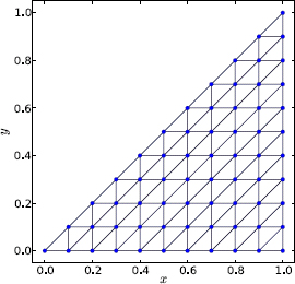
As a test, we apply Program 9.7 to the isosceles right triangular box (see Exercise E9.12). This system is exactly solvable so we can directly compare numerical and analytical results. A sample mesh is shown in Figure 9.15. The isosceles sides are divided into N = 10 intervals each. There are 100 elements. The mesh setup properly preserves the symmetry of the geometry, including reflection symmetry about the bisector of the right angle.
The actual mesh used below is for N = 20, or a total of 400 elements. Of 231 total nodes, 171 are internal, so the dimensions of A and B matrices are 171 × 171, and there are a total of 171 states. The mesh data is stored in a file and is read in by Program 9.7. Figures 9.16 and 9.17 display the eigenenergies and wave functions, respectively, of low-lying states. The latter is obtained from a separate code, Program 9.8, which plots the wave function over a triangle mesh.
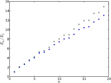
Figure 9.16: The first 20 eigenenergies of the right triangular box. The open circles (![]() ) are FEM results, and filled circles (•) analytic results.
) are FEM results, and filled circles (•) analytic results.
Comparing numerical and analytic eigenenergies, we observe good agreement for the lower states, within ~ 1% for the first 5 states. Analytically, the solutions can be obtained from the 2D box as
![]()
where a is the side length. In Eq. (9.50), m and n are nonzero integers, and m < n. The wave function is a combination of 1D wave functions in the x and y directions (S:8.39), satisfying the boundary condition that the wave function is zero on the three sides, umn(x, 0) = umn(a, y) = umn(x, y = x) = 0. The eigenenergies are given by
![]()
In contrast to the rectangular box which has degeneracies, the triangular box removes degeneracy all together, a result of boundary conditions requiring that the wave function vanish on the hypotenuse. This restricts the way the wave function can oscillate. As Figure 9.17 shows, the ground state has one peak in the center of the triangle. With increasing state number, more pockets are formed, which are generally correlated with the state number, but not always. Sometimes, the pockets are broadly-connected local maxima or minima (e.g., states 3 and 4). They develop into clear peaks at later stages (e.g., states 4 → 5).

The wave function (9.50) in the triangular box is not separable into a product of x and y variables. Therefore, the concept of nodes is not readily applicable. Instead, we must identify the wave function by nodal lines or the pattern of the extrema. A higher number of extrema corresponds to a higher state. If two states have the same number of extrema, the wave function with sharper and better developed peaks belongs to the higher state.
Going back to the eigenenergies shown in Figure 9.16, the discrepancy between the numerical and analytic results increases toward higher states, and numerical values are always above the analytic values for a given state. At the 20th state, the error is about ~ 15%. The difference comes from two sources, the accuracy of the FEM, and the related number of representable states. The difference can be reduced with a finer mesh, which in turn increases the number of states in the FEM representation. This will delay the onset of large errors, but they will happen eventually.
In other words, the fundamental problem remains, which is to represent a system having an infinite number of states with a finite number of representable states in a numerical method. We had seen the same phenomenon for standing waves on a string (Section 6.6). Essentially, we are trying to mimic an infinite Hilbert space with a finite number of states in our basis set. So it is really not the fault of the numerical method. What we must keep in mind is that higher states have larger errors. In the present case, we can trust the energies of states up to 8 at 1% accuracy, or about 5% of the total states (171). A general guide requires a statistical analysis of energy levels (Section S:9.1).
9.6.3 The hexagon quantum dot
The hexagon quantum dot is very interesting. Its shape is highly symmetric, and appears naturally in semiconductors such as GaAs or in a honeycomb as the basic cell.
Figure 9.18 shows a sample mesh of the hexagon quantum dot. The side length, assumed to be 1, is divided into N = 2 intervals for illustration. It is generated with Program 9.9. The elements are equilateral triangles, preserving all the rotation and reflection symmetries. Note that the node number starts from the bottom-left corner and increases consecutively from left to right and bottom to top, until the end of the center row, where it jumps to the top-left corner. This has to do with the way the mesh was made, in which the lower half was generated first and the upper half obtained by reflection (see explanation of Program 9.9).

The number of elements is equal to 6N2. We use more elements than shown in Figure 9.18 in actual computation. We have performed a series of calculations with N = 10 to 40. This is done in part to gauge accuracy and to understand the rate of convergence. In Table 9.3 and Figure 9.19, we show eigenenergies and wave functions calculated with N = 40 and 9600 elements. The hexagon quantum dot does not yield analytic solutions in general. Analytic solutions can be obtained only for a limited subset of highly symmetric states. Even then, they are not in closed form [57]. Judging from the convergence sequence, the relative error in the eigenenergies of Table 9.3 is about ~ 10−3.
The energy spectrum is very interesting. The ground state, which must be nondegenerate, has an energy 3.57866. With regard to geometry, we can compare this value to three wells of comparable size, two circular wells – an inner circular well of diameter ![]() that just fits inside the hexagon and an outer one of diameter 2 that just encloses the hexagon, and a rectangular well of dimensions
that just fits inside the hexagon and an outer one of diameter 2 that just encloses the hexagon, and a rectangular well of dimensions ![]() . The eigenenergies of the circular wells are related to the zeros of the Bessel function, and that of the rectangular well is well known. In order, their values are 3.85546, 2.89159, and 2.87863, respectively (Exercise S:E9.5). The inner circular well gives the best fit to the hexagon, and its energy is the closest. It is higher than the actual energy because its area is smaller than the area of the hexagon. This is due to the uncertainty principle which generally dictates a larger momentum for a smaller well, thus a higher energy. We see the same trend for the outer circular well with an area π and the rectangular well with an area
. The eigenenergies of the circular wells are related to the zeros of the Bessel function, and that of the rectangular well is well known. In order, their values are 3.85546, 2.89159, and 2.87863, respectively (Exercise S:E9.5). The inner circular well gives the best fit to the hexagon, and its energy is the closest. It is higher than the actual energy because its area is smaller than the area of the hexagon. This is due to the uncertainty principle which generally dictates a larger momentum for a smaller well, thus a higher energy. We see the same trend for the outer circular well with an area π and the rectangular well with an area ![]() .
.
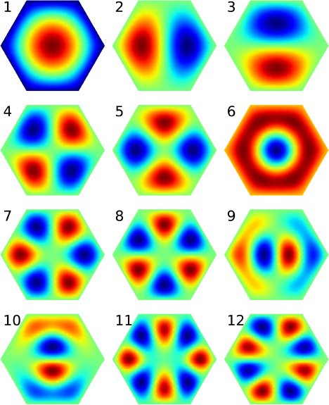
Immediately above the ground state, the first and second excited states are degenerate, as are the next pair, the third and fourth excited states. After states 6 to 8 which are nondegenerate, degeneracy resumes for the next two pair of states, (9, 10) and (11, 12). The pattern continues for later states.
The high frequency of degeneracy is a reflection of the high symmetry of the hexagon structure. It is symmetric under rotations of ![]() about the center, and under reflections about the “diagonals” and bisectors.11 In addition, we can imagine our hexagon is one unit in an infinite honeycomb. Then the system has translation symmetry in several directions. In contrast, the triangular quantum dot discussed earlier lacks these symmetries, and as a result, shows no degeneracy.
about the center, and under reflections about the “diagonals” and bisectors.11 In addition, we can imagine our hexagon is one unit in an infinite honeycomb. Then the system has translation symmetry in several directions. In contrast, the triangular quantum dot discussed earlier lacks these symmetries, and as a result, shows no degeneracy.
Even though the numerical results may have only limited accuracy, the degenerate energies are exactly equal. This is because our mesh preserves the exact symmetry of the system. We expect this symmetry to be carried over to the wave functions.
The corresponding wave functions are shown in Figure 9.19. The ground state has a single maximum as expected. States 2 and 3, which are degenerate, have a peak and a valley each, separated by nodal lines. In state 2, the nodal line runs along a vertical bisector and divides the hexagon into two irregular pentagons. In state 3, it is along the horizontal diagonal and divides the hexagon into two trapezoids. The next pair of degenerate states 4 and 5 have similar saddle-like patterns slightly rotated off each other, but no simple nodal lines. State 4 has two straight nodal lines running along a diagonal and a bisector (like × but in perpendicular directions), while state 5 has two curvy nodal lines running roughly along two bisectors (like χ).
With increasing state number, the patterns become more complex. State 6 has no side-touching nodal lines, but the central peak looks like the peak of the ground state stuck in a bowl. Figure 9.20 compares the two more clearly. The very similar patterns of states 7 and 8 suggest they might be degenerate, but are in fact not. A closer examination of state 8 shows that each of the six peaks or valleys is completely enclosed by an equilateral triangle, so they are the ground state of the equilateral triangle quantum dot. This hexagon state consists of 6 triangular states stitched together. The last two degenerate pairs of states, (9, 10) and (11, 12), show the rapid transition from underdeveloped extrema to sharp peaks and valleys (see Figure 9.20). Electron densities of quantum dots have been imaged experimentally [26], and the single-electron states form the basis for understanding many-electron quantum dots [77].

Figure 9.20: Surface plot of select wave functions from Figure 9.19.
Chapter summary
The focal area of this chapter is the simulation of time-independent quantum systems. We studied systems such as simple wells, linear potentials, central field potentials, and quantum dots. We discussed several methods for solving the Schrödinger equation to obtain the energy spectrum and the wave function. Solutions to any given potential including singular potentials can be found using at least one of the methods presented, making the study of any quantum system within our grasp. Furthermore, each of the methods can be used with minimum modification, at most requiring the user to supply a custom potential function.
With little preparation, we can use the standard shooting method, first introduced for projectile motion, with an ODE solver and a root finder (e.g., RK4 and bisection) to obtain solutions directly. A more efficient approach is to replace the ODE solver with Numerov's method for increased speed and accuracy, while maintaining robustness and versatility.
We also discussed the application of the familiar finite difference and finite element methods previously used for boundary value problems to eigenvalue problems. For 1D eigenvalue problems, the FDM is slightly simpler than the FEM, but has no performance advantage over the FEM. Except for pedagogical reasons, the FEM is preferred because it is able to deal with point potentials.
The basis expansion method can be used as a general meshfree method that depends on the basis functions rather than a space grid since space is not discretized. With an appropriate basis set to a given problem, this method can lead to very accurate solutions even for large systems.
We have devoted considerable effort to the study of quantum dots in this chapter, and developed a full FEM program to solve the Schrödinger equation in 2D for arbitrary boundaries. The program is robust and simple to use, including a small FEM library fem.py that can be used for other general purposes. One may start using the code first, and going through its development after you are familiar with its flow and operation.
Throughout, we have made use of several functions (Airy, Bessel, Hermite, etc.) from the SciPy special function library. We have also discussed file I/O for storing data and avoiding recalculation. Effective graphing techniques have been demonstrated using Matplotlib's triangle plotting capability, which proved to be an excellent fit for working with data over triangular meshes such as in FEM.
9.7 Exercises and Projects
Exercises
| E9.1 | Solve for the eigenenergies of the square well potential shown in Figure 9.1. The eigenequations for even and odd states are given by (in a.u.)
Assume a = 4 and V0 = 4. Also, convert your results to eV and J, respectively. Does it make sense to use the latter? You can find the roots one by one using the bisection or Newton's method, or SciPy's equation solver fsolve (see Exercise E3.8). You may also wish to try SymPy's solver which can find them all at once. Give it a try, see Exercise E3.10. |
| E9.2 | (a) Use the same method as in Exercise E9.1 to compute the eigenenergies of a single-well potential of width (a − b)/2, where a and b are the parameters for the double-well potential (9.6). Compare with the double-well energies in Figure 9.3 using the same parameters.
(b) Shrink the barrier width b by half, and calculate the wave functions with Program 9.2. What happens to the double hump? Predict what will happen to the energy and wave function if the barrier width is increased, but the well width (a − b)/2 is kept the same. Repeat the calculation by doubling b. Discuss your results, and check degeneracy. |
| E9.3 | (a) Verify the first derivative formula (9.60). Subtract the Taylor series y(x ± h) from Eqs. (2.9) and (2.10), keep terms up to h3, and approximate y′″ from Eq. (9.53).
(b) Carry out a von Neumann stability analysis (6.76) for Numerov's method (9.59), and show that it is stable regardless of the step size. Assume a simple function, e.g., f = c. (c) Experiment with instability in unidirectional integration. Pick a correct energy for the single well potential, e.g., the ground state energy from Table 9.1 or Exercise E9.1, integrate the Schrödinger equation from −R to R (or where the wave function diverges badly) with Program 9.1 or 9.2. Plot the wave function. Reverse direction of integration. Discuss your observations. |
| E9.4 | Fill in the steps leading from Eq. (9.12) to (9.13) in 1D FEM. |
| E9.5 | Show that the expectation values of kinetic and potential energies
are given by Eq. (9.19) in terms of the respective |
| E9.6 | (a) Derive the eigenequation (9.24) for the Dirac δ molecule. Divide the space into three regions separated by the δ potentials, apply the boundary condition at x = ±∞, and finally match the wave function at (b) Solve Eq. (9.24) for the symmetric potential (α = β) to express the solutions (9.25) in terms of the Lambert W function. Refer to Chapter 3 (Section 3.4) for an example on the general approach, e.g., after Eq. (3.29). You can also solve it more quickly with SymPy, see Exercise E3.10. |
| E9.7 | A delta-wall potential, shown in Figure 9.21, is composed of a delta potential Show that there exists a bound state only if αa > 1, the same condition for the existence of the excited state in the δ molecule (9.26), and that the energy is also the same (Eq. (9.25), k−). |
| E9.8 | Show that in the BEM, the Schrödinger equation (9.28) can be reduced to Eq. (9.17) with the matrix elements given by Eq. (9.29). Fill in the detail following similar projection methods from Eq. (S:8.24), or from Eq. (9.12) keeping the kinetic energy operator intact, i.e., no integration by parts. |
| E9.9 | Derive the potential matrix element Vmn (9.31) for the square well potential. Show that Vmn = 0 unless m + n is even, in which case
|
| E9.10 | Show that the matrix elements for x, x2, p, and p2 in the SHO basis are
where mj = m + j. The easiest way is to express the position and momentum operators in terms of the raising and lowering operators as
where a0 is the length scale given in Eq. (9.33). When acting on an eigenstate, the operators â and â+ respectively lowers or raises the state by 1 [44],
|
| E9.11 | (a) Given the potential V = β|x|, use variable substitution to arrange the Schrödinger equation (9.1) in the form of Eq. (9.62), the differential equation for Airy functions. Show that the solutions are given by Eq. (9.61).
(b) Match the wave functions at x = 0 and obtain the eigenenergy equations (9.63) for even and odd states, respectively. |
| E9.12 | Use the supplied mesh data file to calculate the eigenenergies and wave functions of the triangle quantum dot with Program 9.7. Compare the eigenenergies with the exact values (9.51) and plot the relative error for all states. Also plot the wave functions of the first 12 states like Figure 9.17 or Figure 9.20. |


Projects
| P9.1 | (a) Run Program 9.1 with E starting below the bottom of the well, say −2V0 < E < −V0. Describe the shape of the wave function and explain why no bound state exists.
(b) Modify Program 9.1 to find the odd bound states. Instead of the derivative being zero at x = 0, the wave function itself is zero. Modify the conditional statement in the main loop to detect the sign change in the wave function. Also add a negative sign to the wave function for x > 0. With the same parameters as in the program, how many odd states are there? Where do the energies fall in relation to the energies of even states? (c) Modify the program so it can find both even and odd states. Double the width of the well, find the number of all bound states (both even and odd). Do the same, but double the depth. Which way is more effective at increasing the number of bound states? Briefly explain. (d) Change the potential to the SHO potential |
| P9.2 | Consider the distorted harmonic potential V(x) = V0 (|x| − x0)2, graphed in Figure 9.22. If x0 = 0, it is the SHO potential. Otherwise, the potential has a double well at x = ±x0, and approaches the SHO potential for large |x| (a) Let (b) Now let x0 = 1.2. Repeat the above calculations. Discuss your results in relation to the SHO energies (x0 = 0). (c) Move the matching point M around, say just below or above x0. Calculate the energy levels for three different M values. Do the energies change? Should they? Why? |
| P9.3 | Modify Program 9.2 to use Numerov's method (9.59). Let the matching point be M. Integrate the Schrödinger equation upward or downward one step beyond M in both directions, so we can calculate the derivative using Eq. (9.60). See Program 9.5.
Profile your code to test the performance gain between Numerov's method and RK45 using the same step size for Project P9.2, for example. Optionally repeat the test for an SHO if the same accuracy is required. |
| P9.4 | (a) Write a program to calculate the eigenenergies in the square well potential using the FDM method. Prepare the (b) The square well is infinitely sharp, but numerically our grid is finite. This causes numerical error if the potential jumps from −V0 to 0 at the walls. Rather than a steep rise, the result can be improved if we linearly interpolate the potential across the edges (see Eq. (3.51), Project P3.2). Modify your potential matrix so that the two values at the grid points immediately outside the well on each side is |
| P9.5 | (a) Evaluate the analytical matrix elements (9.18) for the square well potential. Replace the potential matrix in Program 9.3 by your analytical results. Repeat the calculation to reproduce the results in Table 9.1.
(b) The sharp edges of the square well affects the accuracy of the results. To improve it, linearly interpolate the potential between the two elements bracketing the edges at ±a/2 as
where h is the element size. The interpolated potential is identical to the actual potential outside the zones between the two immediate elements sandwiching the edges. In the zones, it varies linearly from −V0 at |x| = a/2 − h to 0 at |x| = a/2 + h. For best result, set the grid so the edges (±a/2) are also the nodes. Use this potential in Program 9.3 and redo the calculation. Discuss your results. |
| P9.6 | (a) Calculate the energy and wave function of the bound state of the Dirac δ atom. Assume α = 1. Use the FEM code, Program 9.3, and modify the potential matrix so that the only nonzero matrix element is at the node where the δ potential is located. Plot the numerical and analytic wave functions in the same figure, normalize both at the center. Compare numerical and exact results for the energy and wave function.
(b) Check the quality of the wave function near the center. What are the numerical cusp values, u′(0±)/u(0)? How do they compare with the exact value? (c) Calculate the expectation values of kinetic and potential energies from Eq. (9.19). See description of Program 9.3 on how to proceed. (d) Compute the expectation values of 〈x〉, 〈x2〉, 〈p〉, and 〈p2〉. Use the matrix representations of the operators from Exercise S:E9.3 if available. If not, either derive them, or use numerical integration to find 〈x〉 and 〈x2〉. Find the uncertainty ΔxΔp, and verify that it satisfies the uncertainty principle. (e)* Predict and sketch the wave function in momentum space. Calculate and plot the wave function using FFT. Estimate the widths Δx′ and Δp′ from their respective wave functions. Compare Δx′Δp′ with the result above. (f)* Simulate the δ potential with the FDM. Represent the singularity as |
| P9.7 | (a) Using the results from Exercise E9.9, modify Program 9.4 to compute the bound state energies for the square well potential with the box basis set. Also plot the corresponding wave functions.
(b) Calculate the eigenenergy of the Dirac δ-atom using the BEM. Compare with results from Project P9.6 for the same α. Change the number of states N in your basis, and determine the minimum N to achieve a comparable accuracy as the FEM. |
| P9.8 | Study the energy structure of several model central potentials. Choose one potential, and use Program 9.5 as the base code.
(a) First, let us consider a potential that deviates slightly from the Coulomb potential in the power law,
Vary ∈ = 0.01 to 0.1. Compute the energy-level diagram as shown in Figure 9.11. Compare with the hydrogen atom (Z = 1), and summarize the similarities and differences. Note that all states are higher than hydrogen, except the 1s state. Explain why (a figure similar to Figure 9.12 should be helpful). (b) Next, consider the screened Coulomb potential (Yukawa),
The parameter a is the screening length. This potential behaves like the Coulomb potential for r → 0 but has a much shorter range. Let a = 20 and Z = 1. Calculate the energy-level diagram as above. Find the energy difference between 2s and 2p states. Is the number of bound states finite? Double Z = 2, repeat the calculation. Observe the difference with Z = 1. (c) Last, consider the Hulthén potential,
where Z is the nuclear charge, and a the screening length. What is the potential like in the limits r → 0 and ∞? Based on your observations from above, sketch the energy-level diagram. Choose Z = 1 and a = 10, and calculate the energy-level diagram. Find the largest l supported by the potential. Plot the wave function for the s states, and compare both with the hydrogen atom. Examine the number of nodes in the wave function so as not to miss any states. Repeat the calculation for Z = 2, keep the same a. (d)* Modify your program to compute the expectation values of kinetic and potential energies, respectively. Since the wave function is obtained on a regular grid, we can use Simpson's rule (Section 8.A.2) to carry out the numerical integral. For 〈T〉, do not compute the derivatives directly. Rather, use either the first derivative (9.60) in Eq. (8.18), or the second derivative from Eq. (9.8) with the integral in Exercise E9.5. In addition, properly scale your results by C = ∫ u*udx, because the wave function is not normalized. Test your program on hydrogen atom to make sure it gives the correct results according to the virial theorem (9.40). For potentials given above, compute 〈T〉 and 〈V〉 for the lowest state in each l-series. Do they still obey the virial theorem? Comment on your results. |
| P9.9 | (a) Calculate and plot the wave functions of the unit circle quantum dot (billiard, Section S:9.2.1) using the supplied mesh data file. Discuss the symmetry of the degenerate states.
(b) Generate a mesh for the circular billiard so it preserves rotational symmetry within the grid representation. One way to do this is start with the mesh grid of the hexagon or octagon, scale the points off the circle symmetrically about the radial they are on. Calculate the eigenenergies, and compare the degenerate states against Table S:9.1. |
| P9.10 | (a) Generate a mesh for the hexagon using Program 9.9. Plot the kinetic energy matrix (or equivalently the overlap matrix) similar to Figure 7.12. You should see bands running along the diagonal initially, but a little later some bands break, jump away from the diagonal, and continue from there. This is caused by the discontinuity in numbering the nodes due to reflection.
(b) Modify the program so the nodes are consecutively numbered, or post-process the mesh to achieve the same goal. Check the bandedness by plotting the matrix again. (c)* Represent the new matrix in banded matrix format, see Figure 8.6 and Program 8.3. Solve the eigenvalue problem using the SciPy eig_banded() function. Profile your programs and compare speeds between the standard and banded eigensolvers. |


9.A Numerov's method
The Numerov method is useful for a second order ODE of the following form that does not contain first derivatives
![]()
It turns out that we can apply a special technique to discretize it over a grid such that odd derivatives up to the fifth order can be canceled in the central difference scheme, giving us a method accurate to h5, h being the grid size as usual.
To show this, we apply an operator to Eq. (9.53),
![]()
Using the Taylor series for y(x ± h) from Eqs. (2.9) and (2.10) and adding them up, we have,
![]()
![]()
which is accurate to order h4 (compare with Eq. (6.31b)).
Substituting Eq. (9.56) into (9.54), we see that the terms y″″ cancel, leaving us with
![]()
To approximate (fy)″, we can use Eq. (9.56) but keep only the first term so the error is still of the order h4. Switching to the usual subscript notation, Eq. (9.57) becomes
![]()
Solving for yi+1, we obtain Numerov's method

Numerov's method is a three-term recursion relation. It is stable (Exercise E9.3) and has a local error of the order O(h6). This is the same order as the Runge-Kutta-Felhberg method (RK45, Section 2.3.2), which requires six function calls. Numerov's method is more efficient with apparent three calls to f(x), but effectively only one new call because the other two can be reused in subsequent iterations. However, it is not self starting, as two seed values are necessary to get started. Program 9.5 contains an implementation of the method. We will include it in our ODE library ode.py from now on.
We can also obtain the first derivative to a higher order taking advantage of the special form Eq. (9.53). It can be shown that the central difference method leads to (Exercise E9.3)
![]()
The error is two orders smaller than the standard central difference formula (6.31a), and is the same as the standard five point scheme. Equation (9.60) is useful for wave function matching in quantum problems.
We note that the standard Numerov method can be modified so it is applicable to ODEs containing first derivatives. The interested reader should check relevant literature if the need arises.
9.B The linear potential and Airy function
In the wedged linear potential V = β|x|, the wave function can be solved (see Exercise E9.11) in terms of a special function called the Airy function, Ai(x),

The Airy function is defined as a solution to the differential equation [10]
![]()
It has two solutions, the non-diverging regular solution Ai(x) and a diverging solution Bi(x). We are interested in the regular solution Ai(x) which is graphed in Figure 9.23.

Since the potential is even, the eigenfunctions (9.61) have definite even or odd parities. As we have seen (e.g., Figure 9.3), even eigenfunctions must have a local maximum at the origin, u′(0) = 0, and odd ones must have a node, u(0) = 0. Accordingly, the eigenenergies must satisfy
![]()
Let zn and ![]() be the n-th zero of Ai(x) and its derivative Ai′(x), respectively. The eigenenergies can be found from Eq. (9.63) as
be the n-th zero of Ai(x) and its derivative Ai′(x), respectively. The eigenenergies can be found from Eq. (9.63) as
![]()
To find the eigenenergies, we need to locate the zeros of the Airy function. The first several zeros are listed in Table 9.4.

If other zeros are needed, they may be generated from the code below using the SciPy special function library.
On return, zn and zpn contain the zeros of Ai(x) and Ai′(x), respectively. The zeros of Bi(x) and Bi′(x) are in zbn and zbpn, which are of no interest to us here.
9.C Program listings and descriptions
Program listing 9.1: Visual eigenstates in the square well (squarewell.py)
The program assumes a symmetric potential well centered at the origin, and calculates the energies of even states. The function sch() is explained in detail in Section 9.1.2. The range of integration is set to [−R, R] where R should be large compared to the width of the well. The range is divided into 2N intervals (2N + 1 grid points). To display the potential, the NumPy vectorize function is used (line 18), which vectorizes a scalar function so it operates on an input array and returns an output array.
The program scans energy E from −V0 to 0. At each E, we integrate the Schrödinger equation from x = −R to the origin, starting with ψ(−R) = 0 (psi[0]) and a small, arbitrary value for the derivative ψ′(−R) (psi[1]). The wave function for x > 0 is obtained by symmetry via slicing (line 27). We count backward from N −1 to 0 to get the reflected wave function from x = h to R.
For even states, the derivative will be zero at the origin if the energy is an eigenenergy. When the derivative changes sign, we assume a correct eigenenergy has been found. The program terminates when E becomes positive, and we have found all even eigenstates.
Program listing 9.2: Shooting method for double well (qmshoot.py)
The potential function V() returns the double square well potential. The functions sch(), intsch() and shoot() have been explained earlier in the text. The limits xL and xR are coupled to the width of the double well, which we take as the characteristic length of the system.
The main loop iterates through the trial energy in equal increment. When a root is bracketed, it is solved with the bisection method. Once a true eigenenergy is found, the wave function is obtained by integrating inward, and matching at grid M, which should be off-center to avoid the node point for symmetric potentials. The wave function is combined by np.concatenate into one array psix for plotting. Note that the order for the downward wave function is reversed via slicing wfdn[::-1] before the combination, which is scaled (matched) according to Eq. (9.3) afterward. The layout of the plots are assumed to be 2 × 2. For other potentials with more bound states, it should be modified accordingly.
Program listing 9.3: Eigenenergies by FEM (qmfem.py)
This is a general FEM program for 1D potentials. The routine TB_mat() prepares the kinetic energy and basis overlap matrices, both tridiagonal, according to Eqs. (9.16a) and (9.16c) using np.diag (see Program 6.3). The next couple of functions Vij() and V_mat() work together to compute the potential matrix (9.18) as explained in the text.
The main code initializes parameters such as the potential, space range, the number of finite elements, and nodes, etc. It then prepares the matrices for the kinetic energy Tm, overlap B, and the potential energy Vm. The eigenenergies and eigenvectors are obtained with the SciPy sparse matrix eigenvalue solver eigsh (line 40), which is more efficient than the standard eigh routine for large matrices. It works on symmetric real or complex Hermitian matrices. The eigenvalues are returned in E as a 1D array, and eigenvectors in u as a 2D array, in such a way that u[:,i], a 1D array over the space grid, is the eigenvector corresponding to E[i].
In many cases, we are interested in only a select group of eigenvalues, such as the low-lying bound states. It is also faster to solve only for a subset of the eigenvalues. We specify the number of eigenvalues (10 in this case) and the sorting option ’SA’ (lowest value first), so this combination of switches gives us the lowest 10 eigenstates. For larger dimensions, consider the banded eigenvalue solver eig_banded in SciPy for better convergence.
The eigenvector, i.e., the wave function, returned by eigsh is properly normalized with B as the weight (9.20), meaning that the statement
evaluates to 1 for any state i. Therefore, we can readily compute any average such as the kinetic or potential energies (9.19). For example, the kinetic energy of the first state (the ground state) is simply
The function np.dot calculates the scalar product if the arguments are 1D arrays. If one of arguments is a 2D array, it is the same as matrix multiplication. This is the case for dot(Tm, u[:,0]), which returns a 1D array as a result of a square matrix Tm multiplied by a column matrix u[:,0]. A second dot operation computes the scalar product, a single number, from the resultant and the wave function, both 1D arrays.
Program listing 9.4: Eigenenergies by BEM (bem.py)
For a given potential defined by the user, V(), the program calculates eigenenergies using the SHO basis set. It generates the kinetic energy matrix from Eq. (9.36). Since it is banded, we use np.diag to build the diagonal and off-diagonal (±2) bands. The potential matrix is computed using numerical integration. The integrand is defined in uVu() which returns the product ![]() in Eq. (9.29). The basis functions un are evaluated using the Hermite polynomials from SciPy special functions library. You can also switch to the recurrence formula (9.35) to generate your own Hermite polynomials efficiently.
in Eq. (9.29). The basis functions un are evaluated using the Hermite polynomials from SciPy special functions library. You can also switch to the recurrence formula (9.35) to generate your own Hermite polynomials efficiently.
Note that the numerical integral is performed for positive x only and multiplied by 2 to account for the negative x by symmetry. This needs to be modified if the potential is not symmetric. Another caution is in order. If higher basis states are used, the integrand will be highly oscillatory, and the integral may become inaccurate. Make sure to check convergence, e.g., by breaking the interval into two, or varying the upper limit, etc.
The eigenenergies obtained with eigsh are compared with exact values from Eq. (9.64) in terms of the zeros of the Airy function. The odd states are inserted after every even state (line 27).
Program listing 9.5: Hydrogen atom by Numerov's method (hydrogen.py)
The functions Veff() and f() calculate the effective potential and the Schrödinger equation (9.8), respectively. The routine numerov() is a standalone Numerov integrator. It receives f(x) to be integrated as input, together with initial values [u0, u1], number of steps n to advance, starting position x, and step size h. On return, the n new values plus the initial pair are contained in u = [u0, u1, ···, un+1]. The same module is included in the ODE library ode.py for convenience.
The module shoot() works the same way as the one in Program 9.2. It calls numerov() twice to integrate the Schrödinger equation inward from both ends, going one step past the matching point M in each direction (recall the number of steps counts from u1 upward or uN−1 downward). This is so that we can use the three-point formula (9.60) to compute the first derivative at M.
The main code sets parameters including the maximum angular momentum lmax. For each l, the main loop scans the energy range for eigenenergies. When one is found, the principal number n is increased. If no valid eigenenergies are skipped, n − l − 1 is equal to the number of nodes. The energy levels are plotted at the end, grouped by l. The plotting statements for the wave function are similar to those in Program 9.2 and thus omitted.
For large n, l, the code can be modified to use the more efficient logarithmic grid. See Exercise S:E9.2.
Program listing 9.6: FEM library (fem.py)
This FEM library includes the necessary functions for FEM solutions of 2D quantum systems. Two functions are meant to be internal: abg() returning α, β, γ and area of a basis function (7.11) at the three nodes of an element; and overlap() calculating the overlap integral (9.49) between two nodes.
The two external functions, A_mat() and B_mat(), compute the A and B matrices, respectively, as defined in Eqs. (9.48), (7.27), and (9.49). They iterate through the elements, calling the internal functions to compute the contributions from each element, and assigning them to the appropriate matrix entry (see Figure 7.10 and associated discussion). After processing all the elements in this element-oriented approach, all contributions will have been accounted for, and the matrices A and B will be completely built.
Program listing 9.7: Quantum dot (qmdot.py)
This is a universal FEM program for quantum dot calculations. It requires the mesh data file (see Figure 9.24 and its associated mesh file format).
After reading in the mesh data, it tries to check the existence of the eigenvalue data file. If it exists, presumably from a previous calculation, it simply loads the data using the pickle file handler (line 13). This handler is very handy for outputting data to a file. It works with the dump function that can pickle, or package, any data and write it to a file. For our use, it is most convenient to form a tuple of eigenenergies and eigenfunctions (line 23) and dump it in one operation.
If the eigenvalue data file does not exist, indicated by the exception IOError, the program starts a new calculation. Matrices ![]() and B are obtained from the FEM library, boundary nodes are deleted (same as in Program 7.3), and the generalized eigenvalue equation is solved using the sparse eigensolver from SciPy, eigsh. Since we usually do not want all states, we specify the number of states we do want, nt, which must be less than the rank of the matrix, or the number of internal nodes in our case. The results are dumped to the eigendata file, so it can be independently analyzed without repeating the calculation which could be long for large problems. It is possible that pickle can run out of memory storing the data set (E, u) for large matrices. If this is the case, either break up the set into smaller chunks, or storing all eigenenergies and only a subset of eigenfunctions.
and B are obtained from the FEM library, boundary nodes are deleted (same as in Program 7.3), and the generalized eigenvalue equation is solved using the sparse eigensolver from SciPy, eigsh. Since we usually do not want all states, we specify the number of states we do want, nt, which must be less than the rank of the matrix, or the number of internal nodes in our case. The results are dumped to the eigendata file, so it can be independently analyzed without repeating the calculation which could be long for large problems. It is possible that pickle can run out of memory storing the data set (E, u) for large matrices. If this is the case, either break up the set into smaller chunks, or storing all eigenenergies and only a subset of eigenfunctions.
At the end, the program prints the eigenenergies, and inserts the boundary values back into the wave function for graphing, assuming bp is already sorted. The wave function of a chosen state is graphed with the newer function plot_trisurf(x,y,z). It interprets the x, y, and z values as 1D arrays defining the points of triangular patches. It fits our purpose well, and we do not have to regenerate the grid.
If the mesh is such that the system matrices are banded, the program can be modified to use a banded eigensolver, eig_banded. The program could then handle very large matrices efficiently. See Figure 8.6 and corresponding discussion for band matrix representation.
Program listing 9.8: Triangle-mesh plotting of wave function (tripwf.py)
This program plots the wave function over a triangular mesh using the Matplotlib function tripcolor(), which fits our need perfectly with shading. The code requires the mesh data and eigenvectors from Program 9.7 stored in respective files. The boundary points stored in bp must be sorted if meshes generated from other sources are used. As it is, the first 12 states are graphed, but we can change the state list st to graph any states desired.
Program listing 9.9: Hexagon mesh generator (meshhex.py)
We can generate a mesh similar to Figure 9.18 with this program. It starts from the bottom row (yj = 0), going from left to right, and up to the center row (y = 0). The nodes above the center row are obtained by reflection.
Below y = 0, the nodes are enumerated sequentially. Assuming each side divided into N intervals, the node number at row yj and column xi (counting from left) is given by ![]() . This is calculated by ndn defined as a lambda function. Unless at the end of a row, two elements are formed at each node (i, j) in CCW order, the elements above and to the right (note that the row above is effectively left-shifted by one). This is similar to Program 7.3. The boundary and internal nodes are also recorded. The process stops after the center row. The number of nodes below the center row is
. This is calculated by ndn defined as a lambda function. Unless at the end of a row, two elements are formed at each node (i, j) in CCW order, the elements above and to the right (note that the row above is effectively left-shifted by one). This is similar to Program 7.3. The boundary and internal nodes are also recorded. The process stops after the center row. The number of nodes below the center row is ![]() .
.
For the other half above y > 0, we use reflection to copy the nodes below, reversing the sign of y coordinates. This is efficiently done using NumPy array slicing and column stacking (line 22), which puts the same x-column and the negative y-column side-by-side to make a 2D array. The flipped nodes are added (concatenated) to the nodes for y ≤ 0. The elements are also copied over, but nodes 0 and 1 are swapped so they are in CCW order (line 25). An offset is added to the copied nodes so their numbers start after the right-most node of the center row, K = M + 2N + 1. We used array mask, i.e., truth array (line 26, see Section 1.D), to exclude the nodes on the center row. When finished, the total number of elements is 6N2.
Finally, the mesh data is written to a file containing, in order, the nodes, elements, boundary and internal nodes. The elm array is converted to a list via tolist method for easy formating by the file writer. As an example, the format of the file for the mesh shown in Figure 9.24 is illustrated below, which can be read by readmesh().

1The study concluded: “Students … are weaned on continuous, well-behaved functions and variables. It is therefore often a shock to them when they study quantum mechanics and find, suddenly, discrete variables. The purpose of the computer-generated film described in this paper is to illustrate that these discrete variables are not so peculiar after all – that, in fact, they arise in a natural way from requiring the solution of the Schrödinger equation to be continuous, differentiable, and finite”.
2A mathematically equivalent form to Eq. (9.5) is ![]() , but this is not stable for numerical work, because the wave function or its derivative can become close to zero, and f(E) could fluctuate wildly.
, but this is not stable for numerical work, because the wave function or its derivative can become close to zero, and f(E) could fluctuate wildly.
3Owing to the boundary conditions, these positive energy states are bound states in the (numerically finite) box, mimicking the true continuum states of the actual, infinite system.
4This was discussed in Chapter 7 and illustrated in Figure 7.10 for FEM in 2D. The reason is still true in 1D.
5The Dirac δ molecule is a good model for understanding the qualitative features of diatomic molecules such as ![]() , where the terms “gerade” and “ungerade” are used to describe the symmetric ground and the antisymmetric excited states, respectively.
, where the terms “gerade” and “ungerade” are used to describe the symmetric ground and the antisymmetric excited states, respectively.
6The wave functions un are available from SymPy: sympy.physics.qho_1d.psi_n.
7Technically, a particle never becomes free in the Coulomb potential, even though it can escape to infinity if its energy is positive. In this case, the continuum wave function is distorted compared to the plane wave representing a truly free particle. See Section 12.B and Exercise S:E12.7.
8Because 〈r〉 scales like n2, numerical integration must extend to large distances for moderate to large n. To maintain efficiency, numerical integration is often done on a logarithmic grid. See Exercise S:E9.2.
9Quantum dots are literally shining a new light on quantum mechanics. Since the energy levels, hence light emission, can be manually controlled via shape and size, they are beginning to usher in new technologies such as the quantum dot display.
10For other nontrivial potentials, numerical integration is more conveniently carried out by mapping the triangles to a simpler shape such as isosceles right triangles through coordinate transformations.
11Here we ascribe the term “diagonals” to lines connecting the opposite vertices, and bisectors to lines connecting the centers of opposite edges.