
Chapter 11
Thermal systems
Up to the last chapter, we had built simulations from first principles, i.e., calculations were done from Newton's laws or the Schrödinger equation. Thermal systems, however, require a different, statistical approach since they are made up of large numbers of atoms and molecules. Macroscopic thermal properties are determined by the microscopic interactions between these particles. Given that the number of particles is at least on the order of the Avogadro number ∼ 1023, we cannot hope to simulate thermal systems using first-principle calculations by tracking all the individual particles.1 Nor would we want to. Even if their individual properties such as the energies or velocities were available, we would not be able to make sense out of that many particles without statistics. It turns out that we can model much smaller thermal systems and still simulate the statistical properties of large systems, provided we sample them correctly and be mindful of the limitations.
We begin with thermodynamics of equilibrium, exploring the role of energy sharing, entropy, and temperature as the driving forces toward equilibrium: the Boltzmann distribution. We then introduce the Metropolis algorithm and apply it to study 1D and 2D Ising models, carefully comparing numerical and analytic solutions where possible, including phase transitions. After fully assessing the Metropolis method, we extend it to the study of non-thermal systems such as the hanging tablecloth via simulated annealing. Finally, we investigate the thermalization of N-body atomic systems and kinetic gas theory by molecular dynamics, connecting first-principle calculations to thermal properties.
11.1 Thermodynamics of equilibrium
The central idea in statistical thermodynamics is the Boltzmann distribution. It describes the energy distribution of a thermal system, and is the most powerful tool we have in statistical mechanics. In this section we explore the equilibrium process and show, through numerical (Monte Carlo) experiments, that Boltzmann statistics arises naturally in thermal equilibrium as a matter of overwhelming probability.
11.1.1 Toward thermal equilibrium
To understand probabilities of states, we begin with counting of states at the microscopic level. Imagine a thermal system made up of microscopic particles that can store energy internally in translational motion, rotation, or vibration. The specific mechanism is unimportant. For example, consider the Einstein solid model, one of the few analytically solvable problems. The system consists of N independent quantum simple harmonic oscillators (SHO). Each SHO has an infinite number of equidistant states (see Eq. (9.32)), and can store an unlimited quanta of energy. Suppose the system has a total energy of qε with ε as the basic unit of energy. The energy can be shared in many ways among the N oscillators. A microstate refers to a particular distribution of energy.
At the macroscopic level, we are interested in the net, externally distinguishable effects, called macrostates. Consider two microstates in the Einstein solid example: one in which a single oscillator has all q units of energy and the rest N − 1 oscillators have none, and another in which the first q oscillators have one unit of energy each and none for the rest. These two different microstates correspond to the same macrostate, a state of total energy q. In fact, all different microstates of an Einstein solid with a given energy is just one macrostate, irrespective of how it is distributed internally.
As there can be multiple microstates for a given macrostate, the correspondence between microstates and macrostates is not unique. The number of microstates in a given macrostate is called the multiplicity, denoted by Ω. The multiplicity, Ω(N, q), of the Einstein solid for a given N and q, can be found analytically [41, 82] (see Exercise E11.1).
To study equilibrium, let us consider an isolated system composed of two interacting solids, A and B, with NA and NB oscillators respectively, sharing a total of q units of energy, qA + qB = q. We denote a macrostate n as a particular pair of numbers, n ≡ (qA, qB), where qB = q − qA would be fixed for a given qA. The multiplicity of a macrostate n is equal to the product of multiplicities of the two solids,
![]()
It tells us the number of possible ways (microstates) of arranging energies qA and qB within solids A and B, respectively.
To associate the multiplicity with a probability, we invoke the statistical postulate which states that all accessible microstates are equally probable in an isolated system. This is a fundamental assumption in thermal physics.2 With this postulate, we can assert that the probability of finding the system in macrostate n is
![]()
where ΩT = ∑n Ω(n) is the total multiplicity.
We could calculate the probability distribution from Eq. (11.2) (“theory”, Project P11.2), or we could simulate how this happens naturally (“experiment”). We choose the latter. To do so, we consider an asymmetric pair, NA ![]() NB, a small solid A interacting with a large solid B. This simulates the common situation in which a system of interest is in thermal equilibrium with a large environment (the reservoir).
NB, a small solid A interacting with a large solid B. This simulates the common situation in which a system of interest is in thermal equilibrium with a large environment (the reservoir).
It is more convenient to define an Einstein-solid object via object-oriented programming rather than through a function as usual. This object will be used in more than one program. Furthermore, it can be expanded to two interacting solids. This object is defined as follows.
Program listing 11.1: Einstein solid class (einsteinsolid.py)
  1import random as rnd

  3class EinsteinSolid:                                      # Einstein solid object
      def  _init_ (self, N=400, q=10):
  5              self .N = N
              self. cell = [q]*N                            # q units energy per cell
  7
      def _add_ (self, other):                          # combine two solids
  9             self .N += other.N
             self. cell += other.cell
11             return self

13       def exchange(self, L=20):                    # iterate L times
             for i in range(L):
15                   take = rnd.randint(0, self .N−1) # random pair
                   give = rnd.randint(0, self .N−1)
17                   while self. cell [take] == 0:       # find a nonzero−energy cell
                         take = rnd.randint(0, self .N−1)
19                  self. cell [take] −= 1                   # exchange energy
                  self. cell [give] += 1
The function _init_() is called when an object is instantiated to initialize N oscillators and to store their energies in the attribute cell as a list.3 The next function _add_() defines the addition operator so two solids can be combined such that if C = A+B, then NC = NA + NB and the cells (lists) are concatenated (Project P11.2). This is also called operator overloading. The double underscore marks a method as private to a class.
Because all allowed microstates are equally probable by the statistical postulate, we will let the oscillators exchange energy freely and randomly. This is carried out in exchange() which makes a specified number of iterations through the oscillator list. In each iteration, it randomly picks a pair of oscillators for energy exchange using randint(n1,n2), which returns a random integer between n1 and n2, inclusive. After finding an oscillator with a nonzero energy, it takes one unit of energy from that oscillator and gives it to the other. As discussed below, this is equivalent to the interaction between a single oscillator and the rest.
Given an initial state, we allow many interactions to occur to reach equilibrium. We can count the number of cells with a given amount of energy to obtain the energy distribution. What is the distribution after equilibrium is established?

Figure 11.1: The energy distribution of an Einstein solid (256 oscillators) at given iterations (time). The darker the cell, the higher the energy.
We first present results from Program 11.4 for a small Einstein-solid object (256 oscillators) in Figure 11.1, which shows the energy distribution in a 16 × 16 intensity image as a function of iterations elapsed between samplings. Darker cells correspond to higher energies. Not to play favoritism, we give every oscillator the same amount of energy in the initial microstate, indicated by the uniform intensity at the start (first frame). The visual effect clearly shows that, with increasing iterations, the number of white cells increases quickly, followed by ever smaller numbers of lighter to darker gray levels. We get the picture that the most probable states are at low energies.

Figure 11.2: The energy distribution of an Einstein solid (1024 oscillators) at given iterations (time). The smooth curve is an exponential e−αn.
To be more quantitative, we show the results from Program 11.5 in Figure 11.2 for a larger solid with N = 1024. It displays as histograms the relative fraction of oscillators having n units of energy between samplings. Because every oscillator is initialized to one unit of energy, we see a single peak at n = 1 in the first frame. As the number of iterations increases, the distribution widens, and the number of oscillators having zero energy grows rapidly, as observed in the intensity plot Figure 11.1. After 1500 cumulative iterations from the start (the fifth frame), the zero-energy state is the most probable (to check if this might be due to the low initial energy, increase it and run Program 11.5). By the last three frames, the distribution has only small changes. It signals that the system has reached equilibrium, with what looks like an exponential distribution
![]()
Drawing smooth curves through the distribution, we find α ∼ ln 2 gives the best visual fit. We will see why later (Section 11.1.4).

Figure 11.3: The energy distribution in equilibrium (last frame of Figure 11.2) on a semilog scale. The solid line is N(0)e−αn, α = ln 2.
To confirm this, we plot the distribution in Figure 11.3 where N(n) is the number of oscillators having n units of energy, this time on a semilog y scale. The data is from the last frame of Figure 11.2. We can see a clear trend of the data points following closely the exponential function (11.3) which is a straight line on the semilog scale. In addition, we can also see the exponential tail at larger n which is too small to see on a linear scale (Figure 11.2). The error bars are equal to the statistical fluctuation, ![]() . They are produced from Program 11.5 with
. They are produced from Program 11.5 with
plt.errorbar(range(len(bin)), bin, np.sqrt(bin), fmt=None)
In the simulation, we only know the total number of oscillators (N = NA + NB = 1024), but what are the implicit values of NA and NB? From the way we modeled the system, we can interpret the results as caused by the interaction between two solids, NA = 1 and NB = 1023. When we iterated the system, we picked two individual oscillators randomly to exchange energy. Because all oscillators are equivalent, each action is in effect an interaction between a single oscillator (A) and the rest (B). When we plot the histogram, we are effectively plotting the results of N iterations of a single oscillator.
This is the subtlety of the Monte Carlo experiment. We could have focused on a particular oscillator (say the first one), and exchanged energy between it and the rest of the system. Over the long run, we would still have the same cumulative distribution. However, it would be extremely inefficient and would take much longer to obtain results as accurate as these in Figure 11.3.
As we will see shortly (Section 11.1.4), the remarkable “experimental” results, obtained with a system so tiny as to be utterly insignificant compared to a normal thermal system, in fact do agree with Boltzmann statistics in actual systems. Although we used the Einstein solid model, the results are rather general, since the exchange of energy is generic and does not assume any particular mechanism. It illustrates that we can efficiently simulate the behavior of much larger systems using a small but finite model system with correct sampling techniques and proper interpretation. Now we have seen what equilibrium looks like, we try to understand why next.
11.1.2 Entropy
We have seen from above that the thermal system marches from an ordered initial configuration toward somewhat disordered equilibrium configuration. The energy distribution follows a probabilistic course of action given by the exponential factor. The probability is extremely low that the system would spontaneously go back to the ordered initial state, even for our very tiny system of a few thousand oscillators. This all seems purely mathematical.
However, in thermal physics we deal with measurable physical quantities such as energy, heat, etc., not just probability theory. How do we characterize the trend of thermal systems toward disorder? The answer is a physical quantity called entropy.
Entropy measures the degree of disorder, or more precisely, the number of ways a thermal system can be rearranged, namely the multiplicity Ω. Boltzmann defined entropy S as
![]()
where k is the Boltzmann constant. Because the multiplicity Ω is a very large number, the logarithm ln Ω will be a large number. After multiplied by the small k, entropy S will be merely an ordinary number. More importantly, entropy thus defined is additive: the total entropy of a composite system is equal to the sum of individual entropies of its subsystems, because the total multiplicity is equal to the product of multiplicities (11.1).
We can calculate the change of entropy in the above simulation of the Einstein solid. Because we know the probability distributions of an oscillator from Figure 11.2, it is more convenient to calculate entropy using an equivalent expression as [9] (see Section 11.A, Eq. (11.55))
![]()
where Pn is the probability of finding the system in state n.
The function below computes the entropy of one oscillator in the system.
Program listing 11.2: Entropy of an Einstein solid (entropy.py)
  1def entropy(cell):                                 # entropy of Einstein solid
      N, n, nt, s = len(cell), 0, 0, 0.
  3      while nt < N:                                 # until all cells are counted
          cn = cell.count(n)                       # num. of cells with En
  5           n, nt = n + 1, nt + cn                 # increase energy, cumul. cells
           p = cn/float(N)                         # probability
  7           if (cn != 0): s −= p*np.log(p)    # entropy/k, Eq. (11.5)
      return s
It accepts the configuration (microstate) in cell, counts the number of oscillators with energy n (line 4), converts it to a probability, and adds it to the entropy, until all oscillators are accounted for.
We can put the above function in Program 11.5 (or make it a method of the Einstein-solid object in Program 11.1) to obtain the results in Figure 11.4, showing the entropy S of a single oscillator in a system of N = 1024 oscillators, in units of k to make its numerical value tidy. The total entropy of the system is N times larger because it is additive. Initially the entropy is zero because the initial state, where P(1) = 1 and P(n ≠ 1) = 0, is perfectly ordered. As time increases, S grows rapidly, noting the semilog x scale. Near equilibrium at the end, S is maximum and stabilizes to a plateau. Numerical experiments lead us to this observation:

Entropy tends to increase.
This is the second law of thermodynamics [82]. Because entropy measures multiplicity, we can state the second law a little differently: a system in equilibrium will be found in a macrostate of greatest multiplicity (apart from fluctuations).
We can now understand why the most probable state is the ground state (lowest energy state) in terms of entropy. For a given amount of energy, the multiplicity of a macrostate as measured by the entropy is increased by a much greater factor if the energy is deposited in the large system B (reservoir) than in the small system A (microsystem). The energy makes many more microstates accessible in the reservoir than in the microsystem. Using our example NA = 1, NB = 1023 and q = 1, for instance, increasing the energy of system A by one unit has no effect on the number of microstates, it is always 1. But, there are 1023 possibilities, i.e., additional microstates, of distributing one unit of energy in system B. Evidently, of all possibilities, an exponential distribution (i.e., Boltzmann distribution, Section 11.1.4) gives the maximum possible entropy for a system in equilibrium.
11.1.3 Temperature
We intuitively know that when two systems are in equilibrium, they have the same temperature. This leads us to expect that there is a connection between temperature and entropy reaching maximum in the above example.

Figure 11.5: The changes of entropy per oscillator vs. iterations (left) and vs. energy exchange (right) between two equal-sized Einstein solids.
Our small microsystem has very little effect on the temperature of the reservoir because the amount of energy exchanged is limited. We can gain more insight into the equilibrium process by changing the relative sizes of the interacting systems.
Figure 11.5 shows the changes of entropy for two Einstein solids of equal size, NA = NB = 512. We set up the systems so that initially solid A has 3 units of energy per oscillator and solid B has 1. Both are in equilibrium before they are allowed to interact. Once interactions begin, the hotter solid A loses energy more readily than solid B. The change of entropy of A, ΔSA, is negative and decreasing relative to the initial entropy. Conversely, the change of entropy of B, ΔSB, is positive and increasing due to the absorbed energy ΔqB > 0 (Figure 11.5, right). But, the positive gain ΔSB is more than the negative loss ΔSA so the net change ΔST = ΔSA + ΔSB is positive.
Energy will continue to flow from solid A to solid B as long as the net change in entropy is positive. But as the energy transfer continues, the rate of entropy gain decreases. At the point of equilibrium (ΔqB = 512, dashed line in Figure 11.5, right), the net entropy stabilizes and fluctuates. We see the systems reach equilibrium, and their energies are equal qA = qB, apart from fluctuations.

Figure 11.6: The multiplicity (top) and entropy (bottom) of two interacting solids NA = NB = 512, sharing a total energy q = qA + qB = 2048.
The rate of entropy change is an important parameter. From Figure 11.5 (right) we can see that as solid B gains energy, the rate of ΔSB decreases, whereas the rate of ΔSA increases in magnitude, though the clarity of the trends is affected by fluctuations. A clearer picture is given in Figure 11.6 where the total multiplicity and changes of entropy are calculated from Eqs. (11.1) and (11.4) for the same parameters as in Figure 11.5 (Project P11.2). The scaled multiplicity shows a sharp peak near the equilibrium, which would become increasingly narrower for larger systems.
The values of entropy (Figure 11.6, bottom) are relative to a single solid at the beginning qB ∼ 500. The arrows indicate the rates of changes at the beginning and also at the equilibrium (dashed line). When the rates are equal in magnitude, the solids are in equilibrium. Because the total entropy is maximum at that point, we have the equilibrium condition
![]()
We have used qB = q−qA in the last term. Equation (11.6) is a statement on temperature which is the “thing” that is the same for the solids or any systems in equilibrium. Considering that the temperature of a solid rises with increasing energy, we can therefore define the temperature as the inverse of the rate,
![]()
We can see from the slope change in Figure 11.6 that the difference in temperature measures the tendency to give off energy. A body at a higher temperature tends to lose heat, and a body at a lower temperature tends to gain heat. Restated in temperature, the equilibrium condition (11.6) is TA = TB.

Figure 11.7: The temperatures of two interacting solids. The parameters are the same as in Figure 11.6.
Figure 11.7 shows the temperatures from our simulation. We calculate the temperature via the average energy from Eq. (11.13) rather than from the derivative relation (11.7).4 The temperature of solid A steadily decreases while that of solid B increases. The solids reach an equilibrium temperature kT ∼ 2.5ε. The many data points around qB ∼ 1024 indicate the amount of fluctuation. We see the overall trends to be linear to a very good approximation. This is because the average energy 〈E〉 is high. For smaller 〈E〉, the lines would curve (Exercise E11.3).
The entropy in Einstein solids increases with energy (Figure 11.6), accompanied with increasing temperature. This is the normal behavior. However, it is not always the case. For systems such as a paramagnet that can store only a limited amount of energy, the entropy can decrease with increasing energy. The slope ∂S/∂E then is negative. According to Eq. (11.7), we have a negative temperature. What does it mean, though? We leave further exploration of such systems to Project P11.3.
11.1.4 Boltzmann distribution
Through numerical simulations, we have established that the energy distribution in equilibrium is an exponential factor (11.3), and temperature is related to entropy by Eq. (11.7).
We only have to relate α in Eq. (11.3) to temperature (see Section 11.A.1). Comparing Eq. (11.3) with the thermodynamic result (11.51) and noting that En = nε, we find α = ε/kT. So Eq. (11.3) becomes
![]()
This is the Boltzmann distribution. It describes the relative probabilities of states of a system in thermal equilibrium [82].
The 1/Z factor may be determined through normalization of probabilities ∑n P(En) = 1, which yields the so-called partition function
![]()
If we know the partition function Z, we can determine all properties of a thermal system in principle. For example, we can calculate the average energy as a weighted average from Eq. (11.8),
![]()
Heat capacity is another important thermodynamic property. It is defined as
![]()
The heat capacity measures the amount of energy required (or released) to raise (or lower) the temperature of a system by one degree. For numerical work, it is more convenient to use an alternative expression [41]
![]()
where Δ2E is the energy fluctuation (Exercise E11.2).
Many other quantities can be obtained this way. The exponential Boltzmann distribution (11.8) is central to thermodynamics.
As an illustration, we can finally determine why α = ln 2 in Figures 11.2 and 11.3. We expect α is related to temperature, which in turn should be related to the average energy of the system. For an SHO, the average energy is analytically available, and the temperature can be expressed as (see Exercise E11.3, ignoring zero point energy)
![]()
where ε (= ħω) is the unit of energy.
For the Einstein solid in our example above (Figure 11.2), the average energy is 1, 〈E〉 = ε, so α = ln 2. Equivalently, the temperature is kT = ε/ ln 2. We have used this value for the exact Boltzmann distribution in Figures 11.2 and 11.3 that show very good agreement between numerical (“experimental”) and analytical results.
11.2 The Ising model
The Einstein model considered above consists of independent oscillators exchanging energy with each other. Now we discuss a model in which the particles are interdependent, i.e., coupled to each other. The simplest, yet nontrivial, model is the Ising model that can exhibit a range of thermodynamic properties. It is useful for understanding critical behaviors including self-organization in magnetism such as ferromagnetism where magnetic dipole moments align themselves spontaneously in the same direction, giving rise to macroscopic domains of net magnetization. In terms of modeling, the simplicity of the Ising model is ideal for us to clearly highlight the important Metropolis algorithm whose basis rests on the Boltzmann distribution.
11.2.1 The 1D Ising model
We consider the 1D Ising model consisting of N identical spins (dipole moments), {si}, arranged in a chain as shown in Figure 11.8.

Each spin has two possible values: either up si = 1, or down si = −1. The interaction energy between any two spins is represented as
![]()
The parameter ε is the pair-wise energy (coupling). If ε > 0, the interaction favors parallel spins, leading to ferromagnetism. For antiferromagnetism, ε < 0, anti-parallel spins are preferred. The specific value ε depends on the properties of the interaction between atoms, not the direct dipole-dipole interaction. The latter is too weak in comparison to the exchange energies arising from symmetries of the wave functions [76] (e.g., see Eq. (9.7) and Figure 9.3). For our purpose, we assume ε > 0, treating it as the basic energy unit of a ferromagnetic system.
In principle, all pairs interact with each other. To keep with simplicity, the Ising model takes into account only nearest neighbor interactions, neglecting all long-range interactions that are presumably weak. We can express the total energy of the 1D Ising model as the sum of neighboring pairs

Here, the last term involves sN+1, which is undefined. We could just neglect that term, which is justified if N is large. However, a better way to deal with the situation without unnecessary complication is to use periodic boundary conditions,
![]()
In effect, we assume that there were virtual identical copies of the chain to the left and to the right of the actual chain. This also helps to minimize finite size effects in Monte Carlo simulations. Another way to visualize Eq. (11.16) is the Ising chain arranged in a ring. The 1D Ising model is analytically solvable.
11.2.2 Metropolis simulation
To simulate the dynamics of the Ising model, we need to put it in contact with a reservoir at temperature T which we just introduced in Eq. (11.7). The reservoir acts as a large heat bath whose temperature remains unchanged while exchanging energy with the Ising system.
Qualitatively, for a given initial configuration and a specified T, the Ising chain will start exchanging energy by flipping the spins in order to reach equilibrium. If the energy of a microstate as given by Eq. (11.15) is too low, the system will absorb energy from the heat bath. Spins will tend to align anti-parallel to each other so the energy of the system is increased. Conversely, if the energy of the microstate is too high, the system will give off energy to the heat bath. This causes the spins to flip toward parallel alignment.
These parallel and anti-parallel spin flips will continue until, after sufficient time passes, the system reaches equilibrium. Then sporadic flips will still occur, but on average, the two types of flips balance each other out. The system will just fluctuate around equilibrium (see Project P11.4 and Figure 11.26 for an animated Ising model).
The question now is how to simulate this equilibrium process. A direct way is to use importance sampling (Section 10.4) to build up a set of microstates that obey the Boltzmann distribution. We would sample randomly a microstate {si}, record its energy E from Eq. (11.15), and accept it with a probability exp(−E/kT). The problem with the direct method is that the number of microstates is large even for a tiny system. For instance, if N = 1000, the number is already 2N ∼ 10300. Out of the uniformly-sampled microstates, only a very small fraction will be near the equilibrium.5 The direct approach would be highly inadequate, unless the process could be biased toward the equilibrium.
The Metropolis algorithm applies a proper bias to efficiently guide the system into equilibrium and keep it there [62]. It works as follows for the Ising model [41]. Starting from a given microstate, we pick a spin randomly and propose to flip it. Let ΔE be the energy difference caused by the flip. If the flip produces a lower energy, i.e., ΔE < 0, the flip is accepted and microstate changed. The reason is because lower energy configurations are always preferred according to the Boltzmann distribution. If the proposed flip produces a higher energy, ΔE > 0, we do not discard the flip entirely. Instead, we accept it with a probability exp(−ΔE/kT) according to Eq. (11.8). This is to account for thermal fluctuations, for otherwise the system would descend to the lowest possible state monotonically with no fluctuation whatsoever, a behavior contradictory to real systems.
This process is repeated many times. If we started with a configuration having an energy above its equilibrium value, the flips will lower the energy on average, and the Metropolis method will accept the flips. This drives the system toward lower energy configurations closer to equilibrium. The opposite happens if the initial configuration is below the equilibrium. Either way, once equilibrium is reached, the flips tend to raise or lower the energy equally, producing only fluctuations. In this pick-and-go manner, the Metropolis method samples microstates obeying the Boltzmann distribution.
Let us first see how the method works in a simulation and analyze it afterward. As stated earlier, we assume the Ising model is ferromagnetic, and without loss of generality, we can set ε = 1. The temperature is measured in terms of the ratio kT/ε. The Metropolis sampling works as follows:
- Set the initial microstate {si}. In principle, any random configuration will do. But at low temperatures kT < 1, the system takes longer to equilibrate. It is better in practice to start with a cold configuration, i.e., more spins parallel to each other than anti-parallel.
- Pick a spin at random (say the i-th), and calculate the energy difference if the spin is to flip (a trial flip). Rather than calculating the energy anew, it is easier and more efficient to just find the energy difference due to the interaction with the nearest neighbors by

Note, the value of si in Eq. (11.17) is the pre-flip value.
- If ΔE < 0, the trial flip is accepted, set si → −si. Otherwise, draw a random number x. If x < exp(−ΔE/kT), accept the flip and set si → −si; if not, reject the trial flip and keep the microstate unchanged. This is the Metropolis algorithm.
- Repeat steps 2 and 3 until equilibrium is established. As a rule of thumb, each spin should be given a sufficient number of chances to flip, say 10 to 100 (or more, depending on temperature).
Program 11.6 simulates the 1D Ising model with the Metropolis algorithm. The core module, update(), is listed below.
def update(N, spin, kT, E, M):     # Metropolis sampling
  2       i, flip = rnd.randint(0, N−1), 0
      dE = 2*spin[i]*(spin[i−1] + spin[(i+1)%N]) # Eq. (11.17) , periodic bc
  4       if (dE < 0.0): flip=1              # flip if dE<0, else flip
       else:                                    # according to exp(−dE/kT)
  6             p = np.exp(−dE/kT)
             if (rnd.random() < p): flip=1
  8       if (flip == 1):                        # accept
            E = E + dE
10            M = M − 2*spin[i]
            spin[i] = −spin[i]
12        return E, M
The Ising chain (N spins) is stored in the array spin[]. The parameters kT, E, and M are respectively the temperature, energy and magnetization (11.18) of the current state. The module picks a random spin index between 0 and N − 1 (inclusive), and calculates the change of energy ΔE from Eq. (11.17) if it is to be flipped. Note that the periodic boundary condition (i = 0 or N − 1) is automatically enforced via modulo operations. If the change ΔE is negative, the flip is accepted and the flag set accordingly. If not, it is accepted with a probability exp(−ΔE/kT). At the end, the energy, magnetization, and the spin itself are updated if the trial flip is accepted, flip=1.
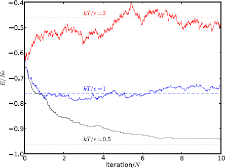
Figure 11.9: The energy of an Ising chain (N = 1000) equilibrating at three temperatures. The dashed lines are the analytic values in equilibrium.
Figure 11.9 shows the energies toward the equilibrium values of an Ising chain with N = 1000 spins as a function of iterations (time). Three temperatures are used: low, kT/ε = 0.5 (ε = 1); intermediate, kT = 1; and high kT = 2. We initialize the system to a configuration whose energy is below the high temperature but above the low and intermediate temperatures. In the beginning, the system rapidly exchanges energy with the heat bath, and quickly approaches their respective equilibrium values from below or above. This is evidenced by the steep slope near the beginning.
In this specific run, the intermediate temperature case (kT = 1) reaches equilibrium first, taking a bit less than one pass (one pass = N iterations, each spin having one chance to flip on average). The quick equilibrium is helped by the initial energy closest to the analytic value for kT = 1.

Figure 11.10: The equilibrium energy (left) and magnetization (right) per spin as a function of temperature. The solid line is the analytic result (11.19).
The high temperature case (kT = 2) rises to its equilibrium level around five passes. In both cases, the energy fluctuates around equilibrium as expected. After a relatively quick initial dive, the rate of energy loss in the low temperature case (kT = 0.5) decreases substantially as the system becomes cooler. The hotter initial state tends to give off energy at a faster rate. But as it cools down, the temperature difference becomes smaller, resulting a slower rate. The system still has not reached equilibrium after ten passes. There is virtually no movement in the last two passes shown. The spins are more tightly aligned, and the chance of flipping to a lower energy is greatly reduced. In this case, only after more than 50 passes did the system reach equilibrium.
After equilibrium is achieved, we can start taking averages. Figure 11.10 displays the results for the average energy and magnetization as a function of temperature. The averages in Monte Carlo Metropolis simulations are calculated as simple algebraic averages. For instance, the average energy and magnetization are
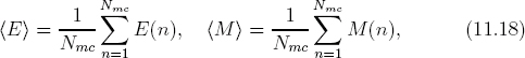
where E(n) is the energy of microstate n (configuration {sn}), computed from Eq. (11.15), and M(n) = ∑i si is the magnetization (net spin). The value Nmc is the total number of Monte Carlo samplings. Because we sample the microstates with the Metropolis algorithm, the importance-sampled microstates obey the Boltzmann distribution. As a result, Eq. (11.18) uses algebraic averages without the explicit weighting factor exp(−E/kT) as would be the case from Eq. (11.10) if the microstates were uniformly sampled. This is a another example of importance sampling (see Section 10.4.2).
The average energy per spin (Figure 11.10) is flat and very close to −1 at T → 0, corresponding to all spins parallel to each other. As seen from Figure 11.9, we must take considerable care to make sure the Ising chain reaches equilibrium at low temperatures before taking averages. The energy grows with increasing temperature, and should approach zero as T → ∞, a state of totally random spin alignment.
The exact energy is given by [82] (Exercise E11.7)
![]()
Overall, we see good agreement with analytic results for the average energy.
For magnetization, the agreement depends on temperature. Theoretically, magnetization is identically zero in the 1D Ising model, even at low temperature when all spins are aligned. The reason is two-fold. First, absent any external magnetic field, there is no preferred direction for the spins. Second, in practically every microstate, a spin can spontaneously flip without changing the total energy. Sometimes this can lead to a domino effect where the spins flip one after another, so the net spin is reversed. The average magnetization is therefore zero.
We see good agreement between numerical and analytic results for magnetization from intermediate to high temperatures (Figure 11.10). But for low temperature kT < 1, numerical data has considerable scatter and the disagreement is large. Increasing the time for equilibrium and for sampling did not seem to noticeably improve the disagreement. On the one hand, most spins are aligned at low T, and there is a low probability of finding a spin with anti-parallel neighbors where a flip requires no extra energy, effectively blocking the most favorable path. On the other hand, a positive amount of energy (11.17) is needed to flip a spin with parallel neighbors, and the probability of accepting the flip is prohibitively low due to the small exponential factor. For example, in such a flip, ΔE = 4. If kT = 0.5, the probability is exp(−ΔE/kT) = exp(−8) ∼ 3 × 10⁻⁴. Basically, the spins are frozen in their alignment at low temperatures, and the time scale for the whole Ising chain to flip is very large. This also happens in actual thermal systems, which can get stuck in a state of finite entropy at low temperatures.

Figure 11.11: The heat capacity per spin as a function of temperature. The solid line is the analytic result.
We show the heat capacity per spin, C(T)/Nk, in Figure 11.11. Numerically, it is calculated from energy fluctuation (11.12) (Project P11.4). The analytic result (solid line) is given by
![]()
Qualitatively, numerical and analytic results behave similarly. The heat capacity is small at low temperature. This is consistent with the average energy (Figure 11.10) which shows only small changes in energy when temperature is varied. At T = 0, C(T) = 0 analytically, a result often attributed to the third law of thermodynamics. At high temperature, the heat capacity again approaches zero as C(T) → 1/T2, since rising temperature is accompanied with little change in energy. In between we observe a maximum at kT ∼ 0.8, corresponding to the change of curvature (bend) in the energy diagram (Figure 11.10).
Quantitatively, the agreement between numerical and analytic results is satisfactory from intermediate to high temperatures (kT ≥ 1). At low temperature, the difference is significant, in line with similar observations for magnetization. For the same reasons as explained earlier, it is tricky to reduce the considerable scatter in the numerical results because of long relaxation times.

Figure 11.12: The entropy per spin as a function of temperature. The solid line is the analytic result.
Finally, we show in Figure 11.12 the entropy of as a function of temperature. To compute the entropy S in the simulation, we use the thermodynamic relationship (11.7)
![]()
We interpret δS as the change of entropy caused by the absorbed energy δE. The results in Figure 11.12 are the cumulative change of entropy, assuming S = 0 at T = 0. Equation (11.21) directly relates entropy to heat and temperature, all experimentally measurable.
The entropy starts from zero, increases quickly between kT = 0.3 and 1, and approaches the asymptotic limit ln 2, i.e., random dipole orientations. The agreement is good between the numerical and analytic results. The latter is given by (Exercise E11.6)
![]()
Comparing entropy (Figure 11.12) with energy (Figure 11.10), the trends are very similar. Upon closer examination of Eq. (11.22), we see the first term dominates at higher temperatures, but has a weaker temperature dependence because of the logarithm. The second term, which is proportional to 〈E〉/T per Eq. (11.19), dominates at intermediate temperatures. As a result, the entropy curve takes on the trend of the average energy at kT ∼ 1, but it levels off faster at higher temperatures due to the 1/T factor.
Summarizing, all thermodynamic quantities presented are continuous and smooth, including energy, magnetization, heat capacity, and entropy. Therefore, the 1D Ising model does not exhibit phase transitions. Per our discussion on magnetization, a spin has only two neighbors in 1D, and the Ising chain can flip-flop freely without energy constraint. It makes critical phenomena impossible in 1D. However, it is possible in 2D Ising model discussed shortly.
The Metropolis algorithm analyzed
We see from above discussions that the 1D Ising model is well described by simulations with the Metropolis algorithm in comparison with analytic results both qualitatively and quantitatively. We wish to analyze more closely the underlying mechanism.
Let E1 and E2 be the energies of two states in a trial transition (flip), and assume E1 < E2. Further, let R(i → f) denote the transition rate from state i to state f. According to the Metropolis algorithm, transitions from states 2 → 1 occur with unit probability, or R(2 → 1) = 1, since it is going from a state of higher energy (E2) to a lower one (E1). Conversely, transitions 1 → 2 has a rate R(1 → 2) = exp(−ΔE/kT) with ΔE = E2−E1. In equilibrium, we expect the number of transitions to be equal in both directions 1 ⇔ 2. Since that number is proportional to the product of the transition rate and the probability of finding the system in the initial state, we have
![]()
where P(E1) and P(E2) are the probabilities of finding the system in states 1 and 2, respectively. Substituting the Metropolis transition rates into Eq. (11.23) we obtain
![]()
This is precisely the Boltzmann distribution (11.8).
Therefore, the Metropolis algorithm leads the system, sometimes slowly but surely, to its correct thermodynamic equilibrium. This algorithm is essential to thermodynamic simulations, and can be adapted to problems that are non-thermodynamic in nature (see Section 11.3).
11.2.3 The 2D Ising model
The 1D Ising model offers many useful insights, but does not exhibit phase transitions. The 2D Ising model addresses this problem. It consists of spins arranged in rows and columns on a lattice, say an N × N square grid for a total of N2 spins (Figure 11.13).

As in the 1D case, we still assume nearest neighbor interactions. Each spin now interacts with four nearest neighbors: up, down, left, and right, doubling the number of nearest neighbors relative to its 1D sibling. The energy for a given microstate is
![]()
where the sum is over all (unique) nearest neighboring pairs, (i, j).
The Monte Carlo simulation of the 2D Ising model runs parallel to that of the 1D Ising model. Let si,j be the spin picked for a trial flip. The change of energy if the spin were to flip is
![]()
This is similar to Eq. (11.17) but with two more neighbors. If the picked spin is on the edge, we use the periodic boundary conditions (11.16) horizontally (column-wise) and vertically (row-wise).
The Metropolis algorithm can be applied in nearly the same manner as before, allowing for minor differences. The equivalent module for the 2D Ising model is given below.
Program listing 11.3: Ising model in 2D (metropolis2.py)
def update2d(N, spin, kT, E, M):     # 2D Ising model, N x N lattice
  2       i, j, flip = rnd.randint(0, N−1), rnd.randint(0, N−1), 0
      dE = 2*spin[i][j]*(spin[i−1][j] + spin[(i+1)%N][j]
  4                                  + spin[i][j−1] + spin[i][(j+1)%N])
       if (dE < 0.0): flip=1                    # flip if dE<0, else flip
  6       else:                                            # according to exp(−dE/kT)
             p = np.exp(−dE/kT)
  8             if (rnd.random() < p): flip=1
       if (flip == 1):
10             E = E + dE
             M = M − 2*spin[i][j]
12             spin[i][j] = −spin[i][j]
       return E, M
Compared to the 1D case (Program 11.6), the only difference is that the spins are stored in a 2D N × N list. To select a spin, we draw a pair of random integers (i, j) representing the column and row indices, respectively. The change of energy is calculated as discussed above from Eq. (11.26). The rest is identical to the 1D case.
Below we discuss simulation results and leave the details of modeling to Project P11.5. We consider a system made up of 1024 spins arranged on a 32 × 32 square lattice. First, we show the spin alignment in Figure 11.14 at several temperatures. Starting from random initial states, the system is sampled after waiting sufficiently long so it has reached equilibrium. The domains may shift depending on when the sampling takes place, but the ratio of “up” to “down” spins should be constant within thermal fluctuations.

Figure 11.14: The Ising square lattice (32 × 32) in equilibrium. Filled squares (![]() ) are “up” spins, and open squares (
) are “up” spins, and open squares (![]() ) are “down” spins.
) are “down” spins.
At the lowest temperature shown (kT = 1), all spins are aligned spontaneously (up). With increasing temperature, more down spins gradually appear. At the higher temperatures kT ≥ 2.8, the numbers of up and down spins are roughly equal, a totally random distribution. However, something dramatic seems to occur between kT = 2.2 and 2.4, which upsets the gradual change in the up/down ratio. The abrupt change is a telltale sign of phase transitions [82].
Phase transitions

Figure 11.15: The energy and magnetization per spin as a function of temperature in the 2D Ising model. The solid lines are the analytic results. The phase transition occurs at Tc = 2.2692 ε/k.
To investigate further, we show the equilibrium energy and magnetization as a function of temperature in Figure 11.15. The energy is continuous and looks qualitatively similar to the 1D case. At low temperature, the energy per spin approaches −2ε, doubling the amount in the 1D Ising model. In 2D, a spin has four nearest neighbors. Since they are all aligned, the total energy is −4ε. Because this energy is mutual between each of the four pairs, the energy per spin is half the total. Another property, difficult to visually spot, is a discontinuity of the slope between kT = 2.2 and 2.4, the same interval observed above (Figure 11.14). Clearly, this is no coincidence.
The magnetization shows that the critical behavior is a phase transition occurring at the critical temperature kTc/ε ![]() 2.2692. Above Tc, the magnetization is identically zero. Below Tc, it rapidly rises to full, spontaneous alignment within a small temperature window.
2.2692. Above Tc, the magnetization is identically zero. Below Tc, it rapidly rises to full, spontaneous alignment within a small temperature window.
The analytic results in Figure 11.15 are given in Section 11.B. The energy and magnetization per spin are [41]
![]()


Figure 11.16: The parameter m (11.57) as a function of temperature. The value of m is 1 at Tc = 2.2692.
The function K(m) in Eq. (11.27) is the complete elliptic integral of the first kind (11.61), and m is a temperature-dependent dimensionless parameter (11.57). The temperature dependence of m is shown in Figure 11.16.
The value of m approaches 1 from both sides of Tc, the critical temperature. However, the function K(1) is infinite because of a logarithmic singularity at m = 1 (Figure 11.27). Because energy must remain finite, we require the factor in front of the second term in Eq. (11.27) to vanish at Tc,
![]()
yielding the critical temperature
![]()
The energy at the critical temperature is ![]() .
.
From the magnetization in Figure 11.15, we see the system undergoing a phase transition at the critical temperature Tc, known as the Curie temperature. Spin orientations are completely random just above Tc, whilst they spontaneously order themselves just below. Note, however, spins of the same orientation tend “stick” together due to the ferromagnetic nature, forming pockets of various sizes like pieces on a go board (Figure 11.14). With increasing temperature, the sizes of the pockets become smaller.
Expanding Eq. (11.28) around Tc, we obtain

The power law scaling like Eq. (11.31) is a common feature in phase transitions. The critical exponent in this case is 1/8. Because the magnetization changes continuously from zero across Tc (even though its derivative is discontinuous), the phase transition may be classified as a continuous one.

Figure 11.17: The heat capacity per spin as a function of temperature in the 2D Ising model. The solid line is the analytic result.
Figure 11.17 displays the heat capacity as a function of temperature. The most prominent feature is the sharp spike at the critical temperature, another sign of possible phase transitions. Unlike energy, there is no requirement that the heat capacity be finite. The critical behavior around Tc can be derived from the analytic expression (11.60),
![]()
This is a logarithmic discontinuity of the derivative of energy. The agreement between simulation and analytic results are good in regions away from the singularity around Tc. Near the singularity, the fluctuations in energy is large, resulting in larger scatter in the heat capacity.
We can now compare the 1D and 2D Ising models and understand why the 1D model does not show phase transitions. In 1D, we can reverse the whole spin chain without energy cost. The initial spin flip may require some extra energy, but it is given back at the end. This is always possible at finite temperatures. The exception is T = 0, when the spins are fully aligned. The Ising chain cannot reverse direction spontaneously without additional energy.
In the 2D model, a spontaneous full reversal of the lattice is not possible once the temperature is below some critical value when net magnetization becomes none zero. On average, additional energies are required to get the process going due to the constraints of the domain walls and neighbors. For instance, consider one row of the spin lattice, the equivalent of a 1D spin chain. This row cannot flip spontaneously because of the interactions with the rows just above and below.
Finally, we discuss finite-size (or edge) effects. All of our results have been obtained with a square lattice of 32 × 32, tiny compared to realistic systems. In most cases, our results are in good agreement with analytic results for N → ∞. We conclude that finite-size effects are small except near phase transitions. Certainly, periodic boundary conditions help to minimize these effects. Nonetheless, we expect the accuracy to improve with larger systems in the region surrounding the phase transition.
In Figure 11.18, we show a larger Ising model containing 1048576 spins on a 1024 × 1024 square lattice at the critical temperature Tc = 2.2692. The initial microstate was hot with random spin directions. The snapshot was taken when equilibrium was well established after each spin had on average 3000 chances to flip, roughly 3 × 10⁹ iterations. The energy of the sampled state is −1.399, within ∼ 1% of the analytic value ![]() . The error remains stable. Analytically, the magnetization should be zero, compared to the sampled value −9.7 × 10⁻⁴. It means that only about 500 spins need to flip to achieve a perfect zero magnetization. Generally, the sampled magnetization has a higher fluctuation than energy, typically in the range ±0.02.
. The error remains stable. Analytically, the magnetization should be zero, compared to the sampled value −9.7 × 10⁻⁴. It means that only about 500 spins need to flip to achieve a perfect zero magnetization. Generally, the sampled magnetization has a higher fluctuation than energy, typically in the range ±0.02.
We again see the tendency of parallel spins sticking together as the lattice is covered by large connected domains (continents), some spanning the full extent of the lattice. In the limit N → ∞, the continents grow to infinity. But there are also smaller islands of varying sizes down to single sites, coexisting with the continents.

Figure 11.18: Snapshot of a 2D Ising model on a square lattice (1024 × 1024, 1048576 spins) in equilibrium at the critical temperature Tc = 2.2692.
11.3 Thermal relaxation by simulated annealing
As the previous examples illustrate, a thermal system at high temperatures will typically be energetic and well mixed. As temperature decreases, it will become more ordered (homogeneous) and equilibrate toward a lower energy state. In the limit T → 0, the system should approach the ground state, provided the temperature decreases gradually. This can take a long time.
This thermal relaxation occurs naturally in many processes such as annealing in materials. For example, heating a metal to higher temperatures and cooling it slowly can improve its structure and properties. Heating helps atoms to mix up with their neighbors, and gradual cooling ensures that they have enough time to find the lowest possible energy states and the most stable structure.
We can simulate the annealing process with the Metropolis method. There are many applications in which simulated annealing is useful and where the problems may not be thermodynamic in nature, including minimization problems in particular where finding the global minimum is essential. In these problems, we first find the equivalent parameters that play the role of energy and state (configuration), then apply the Metropolis method, starting from high to low temperature. At each temperature, sufficient time (Monte Carlo samplings) is allowed for equilibration. The temperature is then lowered, and the process is repeated. Hopefully, the system will be gradually brought to the lowest possible state at the lowest temperature. Below we discuss an example (more examples can be found in Section S:11.1).
The falling tablecloth revisited
Let us revisit the relaxation of a free hanging tablecloth discussed in Section 6.8, where it was modeled as a square array of particles (Figure 6.20) connected by springs.
The relaxation problem was solved by integrating equations of motion in Section 6.8. If we treat it as a thermal process, it is essentially a minimization problem. Given a system of N × N particles of mass m on a square lattice of side L, suspended from the corners, and connected via springs of relaxed length l and spring constant k, what is the minimum energy of the system?

Figure 11.19: Snapshots of a hanging tablecloth in thermal relaxation. Starting from a flat surface (upper left), the temperature decreases in clock-wise order, ending at kT/ε = 10−7 and a minimum energy −2.718ε.
To solve this problem by simulated annealing, we randomly select a particle at grid (i, j). We then jiggle it slightly, causing a displacement of ![]() , and a new position vector of
, and a new position vector of ![]() . We assume the (x, y) coordinates in the horizontal plane, and z in the vertical plane. The change of potential energy (see also Eq. (S:11.1)) for this proposed move is
. We assume the (x, y) coordinates in the horizontal plane, and z in the vertical plane. The change of potential energy (see also Eq. (S:11.1)) for this proposed move is
![]()
where n denotes the nearest neighbors at (i±1, j) and (i, j±1), ![]() is the new distance to the neighbor n, and dn the original distance.
is the new distance to the neighbor n, and dn the original distance.
Having found ΔE, it is straightforward to implement the Metropolis method (Project P11.6). We show the results in Figure 11.19 for a 13 × 13 = 169 particle system. The parameters k, l, and m are the same as in Program 6.8.
We start from the flat configuration (Figure 11.19, upper left, E = 0) at T = 10−3 (set ε = 1 as usual). The next state (upper right) was taken after a few passes so the system is not in equilibrium yet. Its energy is becoming negative, but the surface is rather rough. Temperature is decreased in clockwise order, and the next two states (lower right and left) are snapshots in equilibrium at T = 5 × 10⁻⁴ and 10−7 respectively. The energy changes very little after the last state. The final energy is −2.718ε. Though the exact solution is unknown, it should be very close to the global minimum energy.
Compared to the direct integration method (Figure 6.21, Section 6.8), simulated annealing is simpler to implement, but is slower to converge to the global minimum. In direct integration, if the damping coefficient is chosen properly (at critical value), the system can relax to the global minimum quickly. There is no single parameter in simulated annealing to control this rate. It is the nature of thermal systems that changes occur very slowly at low temperatures. But simulated annealing is more efficient at exploring a larger parameter space and can be applied to solving very difficult problems such as the traveling salesman problem (Section S:11.1).
11.4 Molecular dynamics
We began this chapter by choosing statistical methods over first-principle calculations. Now we return to the latter for molecular dynamics which simulates the motion of N-body systems (atoms or molecules) classically. Because the masses of atoms are much larger than the electron mass (∼ 2000 times), the motion of an atom can be adequately described classically by Newton's laws at all but very low temperatures.
The reason for first-principle molecular dynamics simulations is not to replace statistical mechanics but to complement it. For instance, if we wish to study kinetic and thermal properties of gases such as Maxwell speed distributions (Section 11.4.4), we can use molecular dynamics to follow the motion of each atom classically and obtain thermal properties statistically.6 Furthermore, many systems such as molecular protein or motor simulations involve thousands to millions of atoms in non-equilibrium motion, and molecular dynamics is a very useful tool. It can be used to study atomic and chemical structures or reactions because the internuclear degrees of freedom are effectively separated from the electronic degrees of freedom.
11.4.1 Interaction potentials and units
In a sense, molecular dynamics, an N-body problem, is an extension of the few-body problems discussed in Chapter 4. For instance, we can generalize the three-body equations of motion (4.42) to an N-body system as
![]()

where ![]() is the force between atoms i and j. We typically consider systems of identical particles, so the mass mi = m will be the same for all N atoms.
is the force between atoms i and j. We typically consider systems of identical particles, so the mass mi = m will be the same for all N atoms.
Unlike gravity, the forces ![]() are Coulombic in nature, and there are no exact expressions for them due to many-body interactions (electrons and nuclei). For practical reasons, we use phenomenological forces that approximate the interactions between atoms, including the Morse potential (9.37) (Figure 9.10) and the Lennard-Jones potential (Project S:P9.3). The latter is a two-parameter empirical potential popular among chemists and commonly used in molecular dynamics simulations
are Coulombic in nature, and there are no exact expressions for them due to many-body interactions (electrons and nuclei). For practical reasons, we use phenomenological forces that approximate the interactions between atoms, including the Morse potential (9.37) (Figure 9.10) and the Lennard-Jones potential (Project S:P9.3). The latter is a two-parameter empirical potential popular among chemists and commonly used in molecular dynamics simulations
![]()
where V0 is a positive constant and r0 the equilibrium internuclear distance (Figure 11.20). The first term, 1/r12, describes the strong repulsive wall for r ![]() r0 where the electrons repel each other (Coulomb and Pauli exclusion), but the 12th power law is chosen more for convenience than for fundamental significance. The second term, 1/r6, describes the long-range attraction between neutral atoms due to dipole-dipole interactions (van der Waals force).7 The switch-over between repulsive and attractive forces occurs at r0, where the potential is minimum at −V0.
r0 where the electrons repel each other (Coulomb and Pauli exclusion), but the 12th power law is chosen more for convenience than for fundamental significance. The second term, 1/r6, describes the long-range attraction between neutral atoms due to dipole-dipole interactions (van der Waals force).7 The switch-over between repulsive and attractive forces occurs at r0, where the potential is minimum at −V0.
The force on atom i by atom j is equal to the gradient −∇V,

where ![]() is the relative position vector between atoms i and j, and
is the relative position vector between atoms i and j, and ![]() is the magnitude. As Figure 11.20 shows, the force behaves qualitatively similar to the potential, a sharply rising (1/r13) repulsive force for small r and a rapidly decreasing (1/r7) attractive force for large r. In between, the force is most negative at r = (13/7)1/6r0 ∼ 1.11r0, slightly larger than the equilibrium distance, with the value f ∼ −2.69V0/r0. This force is effective within a small radius r/r0
is the magnitude. As Figure 11.20 shows, the force behaves qualitatively similar to the potential, a sharply rising (1/r13) repulsive force for small r and a rapidly decreasing (1/r7) attractive force for large r. In between, the force is most negative at r = (13/7)1/6r0 ∼ 1.11r0, slightly larger than the equilibrium distance, with the value f ∼ −2.69V0/r0. This force is effective within a small radius r/r0 ![]() 2, and is negligible for larger values r/r0
2, and is negligible for larger values r/r0 ![]() 3. It is a short-ranged force. We will use Eq. (11.37) in the equations of motion (11.35).
3. It is a short-ranged force. We will use Eq. (11.37) in the equations of motion (11.35).

Like before, we need to choose a convenient unit system for the problem at hand. We could use atomic units (Table 8.1), but it is unwieldy as the mass would be unnaturally large, and velocities and energies very small. Since we will be using the Lennard-Jones potential, we shall define energy in units of V0, length in units of r0 as listed in Table 11.1.
Like the unit system for restricted three-body problems (Table 4.3), Table 11.1 is also a floating unit system whose absolute scale is determined by the Lennard-Jones parameters and the mass of atoms. In this sense, simulation results with this unit system are universal. It is particular tidy now for numerical work, for we can just drop V0, r0 and m from Eqs. (11.37) and (11.35). For example, the parameters for argon are V0 = 0.01 eV, r0 = 3.9 Å, and m = 40 amu (6.7 × 10⁻²⁶ kg). The other derived units are: velocity, v0 = 150 m/s; time, t0 = 2.5 × 10⁻¹² s; temperature T0 = 120 K; and pressure P0 = 2.7 × 10⁷ Pa = 270 atm.
11.4.2 Periodic boundary conditions
There is just one more problem before we start writing the program, and it is this: what boundary conditions to use? In actual thermal systems, there are around 1023 particles. Collisions among the particles determine the thermal properties of the systems. Boundary effect are negligible, for we know that air in a ball, a bottle, or a box behaves the same way. We cannot possibly keep track of that many particles. However, we have seen that it is possible to simulate behaviors of real thermal systems with much smaller model systems if we are careful with boundary conditions.
Suppose we set up the system in a cube, for instance, and let the atoms interact and move about. Some atoms will eventually collide with the walls. To prevent them from escaping, we could calculate the point of collision and reflect the atom off the wall elastically, as was done in the stadium billiard problem (Section S:5.1). For a few hundred or thousand particles, collisions with the boundaries will be much more frequent than collisions between the particles themselves. So the boundaries will artificially affect the behaviors, contrary to how real systems behave.
It turns out that, again, we can call on periodic boundary conditions to come to the rescue. We imagine that identical cubes containing identical but virtual systems surround our central cube [42]. For every atom moving in our system, there is an atom with exactly the same position (relative) and velocity in every other virtual cube (Figure 11.21). If an atom escapes our cube, say from the right side (Figure 11.21, atom ![]() ), another one (
), another one (![]() ) enters from the left side to replace it. This way, we do not have to worry about collisions with the walls, because there are no collisions, and we never lose atoms. When a particle exits the cube on one side, it is “teleported” to the opposite side (
) enters from the left side to replace it. This way, we do not have to worry about collisions with the walls, because there are no collisions, and we never lose atoms. When a particle exits the cube on one side, it is “teleported” to the opposite side (![]() , Figure 11.21) without altering its velocity.
, Figure 11.21) without altering its velocity.
But teleporting atoms this way creates another problem. As Figure 11.21 illustrates, the distance between atoms ![]() and
and ![]() changes abruptly when the former is teleported, from r to r′. This causes a discontinuous and unphysical jump in the potential energy and the force. Worse, the teleported atom can exert such a strong, and sudden, force on the atoms already in the close vicinity of its new position that some can be ejected from the system in just a few steps due to numerical error, causing the system to disintegrate.
changes abruptly when the former is teleported, from r to r′. This causes a discontinuous and unphysical jump in the potential energy and the force. Worse, the teleported atom can exert such a strong, and sudden, force on the atoms already in the close vicinity of its new position that some can be ejected from the system in just a few steps due to numerical error, causing the system to disintegrate.

Figure 11.21: Periodic boundary conditions in molecular dynamics simulations. The central real box is surrounded by virtual copies all around.
A careful look of Figure 11.21 between the real atom ![]() and the virtual atom
and the virtual atom ![]() (in the right box) reveals that if we use the distance r′ instead of r, we can avoid the discontinuity in the force. It suggests that we should use the smaller of the two horizontal separations,
(in the right box) reveals that if we use the distance r′ instead of r, we can avoid the discontinuity in the force. It suggests that we should use the smaller of the two horizontal separations, ![]() and
and ![]() , between the atoms. Physically, this means that an atom always finds another atom, be it a real atom or a virtual clone, that is closer along a given axis to interact with. Let us call this close-neighbor interaction.
, between the atoms. Physically, this means that an atom always finds another atom, be it a real atom or a virtual clone, that is closer along a given axis to interact with. Let us call this close-neighbor interaction.
Examination of Figure 11.21 shows that, within close-neighbor interaction, the largest horizontal or vertical separation between two atoms (real or virtual) is equal to half the width of the box. For example, if we shift ![]() horizontally between
horizontally between ![]() and
and ![]() , the largest separation occurs when
, the largest separation occurs when ![]() is exactly in the middle of the two atoms.
is exactly in the middle of the two atoms.
Let L be the width of the box, and Δx = x1 − x2. If ![]() , we accept it as is. But if
, we accept it as is. But if ![]() , we require the following correction
, we require the following correction
![]()
Similar relationships hold for y and z directions.
With the simple and elegant periodic boundary conditions (11.38) as described above, we solve both the boundary-wall collision problems and the abrupt jumps in interaction energies and forces. There is one drawback, however. At exactly ![]() , the force is ambiguous. Using atom
, the force is ambiguous. Using atom ![]() as the example (Figure 11.21), the force would change sign depending whether it interacts with
as the example (Figure 11.21), the force would change sign depending whether it interacts with ![]() to the left or with the virtual clone,
to the left or with the virtual clone, ![]() , to the right. We justify this situation by arguing that, for a box size L
, to the right. We justify this situation by arguing that, for a box size L ![]() r0, the forces between atoms separated at
r0, the forces between atoms separated at ![]() are small as to be negligible. For the Lennard-Jones potential (Figure 11.20), this is true to a very good degree of approximation since the force is short-ranged and is negligible for r
are small as to be negligible. For the Lennard-Jones potential (Figure 11.20), this is true to a very good degree of approximation since the force is short-ranged and is negligible for r ![]() 3 as stated earlier (Figure 11.20). Take L = 10, for instance, the magnitude of the force at
3 as stated earlier (Figure 11.20). Take L = 10, for instance, the magnitude of the force at ![]() is ∼ 10−4. In this case, we expect that the periodic boundary conditions should work well.
is ∼ 10−4. In this case, we expect that the periodic boundary conditions should work well.
Of course, if there were significant spurious effects arising from the use of Eq. (11.38), we would need to amend our approach. Fortunately, Eq. (11.38) works well for molecular dynamics simulations using potentials that decrease rapidly for large r as does the Lennard-Jones potential.
11.4.3 Simulation and visualization
We can now write a molecular dynamics program employing periodic boundary conditions. Taken from the complete Program 11.7, the heart of the simulation computing the core N-body dynamics is given below.
  1def nbody(id, r, v, t):                                 # N−body MD
      if (id == 0):                                        # velocity
  3            return v
      a = np.zeros((N,3))                             # acceleration
  5      for i in range(N):
            rij = r[i]−r[i+1:]                             # rij for all j>i
  7            rij [rij > HL] −= L                         # periodic bc
            rij [rij < −HL] += L
  9            r2 = np.sum(rij*rij, axis=1)           # |rij|ˆ2
            r6 = r2*r2*r2
11            for k in [0,1,2]:                             # L−J force in x,y,z
                   fij = 12.*(1. − r6)*rij [:, k]/(r6*r6*r2)
13                   a[i,k] += np.sum(fij)
                   a[i+1:,k] −= fij                       # 3rd law
15       return a
The module nbody() returns the equations of motion (11.34) and (11.35) in the required format for leapfrog integration. The variables r and v are arrays of vectors, effected by 3-element NumPy arrays, containing the positions and velocities of the atoms. If id=0, velocities are returned. Otherwise, acceleration is calculated in an optimized manner with NumPy arrays.
For a given atom i, we obtain the forces, ![]() , between it and all higher-numbered atoms j = i + 1 to N (of course j ≠ i, an atom does not exert forces on itself). The forces
, between it and all higher-numbered atoms j = i + 1 to N (of course j ≠ i, an atom does not exert forces on itself). The forces ![]() are found by Newton's third law, reducing computation by half. The cumulative effect is that for atom i we only need to find
are found by Newton's third law, reducing computation by half. The cumulative effect is that for atom i we only need to find ![]() for j > i since the other forces (j < i) had been found already in prior iterations. For instance, when i = 1, forces
for j > i since the other forces (j < i) had been found already in prior iterations. For instance, when i = 1, forces ![]() ,
, ![]() , etc., will be calculated. When i = 2, forces
, etc., will be calculated. When i = 2, forces ![]() ,
, ![]() , etc., are needed, but
, etc., are needed, but ![]() was already available and recorded and need not be recalculated.
was already available and recorded and need not be recalculated.
Normally, one would need an explicit inner loop over j, but we avoid it for the sake of speed. We first find the relative position vectors (line 6) ![]() between i and all j > i, simultaneously. Here,
between i and all j > i, simultaneously. Here, ![]() is broadcast into a (N − i − 1) × 3 array (shape of r[i+1:]), equivalent to itself duplicated N − i − 1 times, and then
is broadcast into a (N − i − 1) × 3 array (shape of r[i+1:]), equivalent to itself duplicated N − i − 1 times, and then ![]() for j > i is subtracted from it via element-wise operations. Next, the components of
for j > i is subtracted from it via element-wise operations. Next, the components of ![]() are checked for periodic boundary conditions (11.38) to ensure close-neighbor interactions. This is accomplished with truth array indexing (see Section 1.D, Section 4.4.2), so that separations greater than L/2 in any direction (e.g., |xij | > L/2) are mapped according to Eq. (11.38), again all at once. The distances squared between the atoms are obtained by summing |rij|2 over the three directions via np.sum along the second axis, i.e., across columns (line 9). It is slightly faster to compute r6 and r14 from r2 using multiplications rather than powers (r**n) which is slower for low n.
are checked for periodic boundary conditions (11.38) to ensure close-neighbor interactions. This is accomplished with truth array indexing (see Section 1.D, Section 4.4.2), so that separations greater than L/2 in any direction (e.g., |xij | > L/2) are mapped according to Eq. (11.38), again all at once. The distances squared between the atoms are obtained by summing |rij|2 over the three directions via np.sum along the second axis, i.e., across columns (line 9). It is slightly faster to compute r6 and r14 from r2 using multiplications rather than powers (r**n) which is slower for low n.
Finally, each component of the net force on atom i due to atoms j > i is summed up, and the same component on atom j due to i is obtained via Newton's third law. On exit, accelerations are returned as an N × 3 array of vectors.
Figure 11.22 shows two snapshots of an animated molecular dynamics simulation. We used N = 16 atoms, initially randomly distributed in a cube of side length L = 10. The initial velocities were set randomly between [−1, 1]. We can see from the trails that close-by atoms interact strongly (sharp turns), and distant ones interact weakly (nearly straight line trajectories). In particular, the dark-colored (red) atom (Figure 11.22, left) suffers a strong force near the beginning, being close to several atoms to the right. It makes a sharp turn toward the left wall. After a short time, it exits the cube, and re-enters from the right side by the periodic boundary conditions. For the duration shown between the two frames, this is the only atom escaping the cube. But several atoms near the top and back in the second frame are just about to exit the cube. When they do, the same periodic boundary conditions will be applied, and they will continue to interact with other atoms without collisions with boundary walls.

Figure 11.22: Animated molecular dynamics simulation. The left-most particle (red/dark color) in the left frame exited the cube and is wrapped around by periodic boundary conditions (right frame).
11.4.4 Maxwell distributions and kinetic properties
We can obtain a slew of properties by analyzing relevant data. We show only results and leave the work to Project P11.7. All results are in the floating-scale units (Table 11.1). Figure 11.23 displays the velocity P(vx) (similar for vy and vz) and speed P(v) distributions. We divide the velocity and speed ranges into certain number of bins. Data is sampled periodically (say every 20 time steps). Each time, the atoms are added to the appropriate bins according to their velocities and speeds. The cumulative results are plotted as histograms in Figure 11.23, normalized to one at the maximum.
The results are broken down into three time intervals to show the distribution at different stages of evolution. Toward the beginning (t = 0 to 10), the initial conditions are heavily weighted with large scatters. By the second interval 10 to 50, the distributions look more and more like the equilibrium Maxwell velocity distribution [82]

Figure 11.23: Velocity (left) and speed (right) distributions for N = 40 atoms. Data are taken in different time intervals: •, t = 0 to 10; ![]() , 10 to 50;
, 10 to 50; ![]() , 50 to 400. The solid curves are the Maxwell distributions.
, 50 to 400. The solid curves are the Maxwell distributions.
![]()
and the speed distribution
![]()
Roughly speaking, Eqs. (11.39) and (11.40) are a result of the Boltzmann distribution (11.8), with ![]() and
and ![]() , respectively. The prefactor 4πv2 in Eq. (11.40) comes from the volume element d3v = 4πv2dv.
, respectively. The prefactor 4πv2 in Eq. (11.40) comes from the volume element d3v = 4πv2dv.
In the last interval (50 to 400), the results are in very good agreement with the respective Maxwell distributions, including the symmetry about zero in the velocity distribution, and the forward-backward asymmetry about the maximum in the speed distribution. This indicates that the system has reached equilibrium for t ![]() 50. Considering that we have only N = 40 atoms in the simulation, the convergence is quite fast, a big factor due to the use of periodic boundary conditions.
50. Considering that we have only N = 40 atoms in the simulation, the convergence is quite fast, a big factor due to the use of periodic boundary conditions.

Figure 11.24: The average of speed squared as a function of time. The system is the same as in Figure 11.23.
The equilibrium temperature is determined by the energy of the initial condition. The average kinetic energy is related to temperature by the equipartition theorem: a quadratic degree of freedom carries ![]() of energy [82]. An atom has three translational degrees of freedom in 3D, so its average kinetic energy is
of energy [82]. An atom has three translational degrees of freedom in 3D, so its average kinetic energy is
![]()
We can obtain the equilibrium temperature from Eq. (11.41). Figure 11.24 shows the speed squared as a function of time. It is calculated periodically by averaging the speed squared v2 of all atoms at once. The average value of v2 rises steadily in the beginning, indicating an oversupply of potential energy in the initial condition. It quickly reaches a plateau around 〈v2〉 ∼ 1.85 at t ∼ 40, consistent with the equilibration time observed from Figure 11.23. Using this value, the temperature from Eq. (11.41) is kT = 〈v2〉/3 = 0.62. We have used this temperature in the Maxwell velocity and speed distributions in Figure 11.23.
There is considerable fluctuation in v2. The main cause is due to the small number of atoms. During motion, some atoms can “bunch” up, creating local concentrations that have higher or lower than normal potential energies. As a result, kinetic energies rise or fall accordingly, leading to the observed fluctuations.

Figure 11.25: The number of collisions (left) and the average pressure (right) as a function of time. The system is the same as in Figure 11.23. The solid curve shows the expected pressure for an ideal gas at kT = 0.62.
We can also obtain pressure from our simulation (Figure 11.25), even though using periodic boundary conditions we have managed to avoid any atom-wall collisions, which generates pressure in real systems. Pressure is calculated as follows. When an atom escapes the cube, say from the side, we record its velocity vx before teleporting it. We assume that, as in a real system without periodic boundary conditions, the atom would be spectrally reflected from the wall, reversing the x velocity to −vx. The change of momentum (impulse) would be Δpi = −2mvx. We keep cumulating the impulse within a given time interval Δt (e.g., 20 time steps). The force exerted on the wall would be F = ∑iΔpi/Δt, which yields the pressure, P = F/L2.
Figure 11.25 shows the number of collisions per Δt = 0.2 (left) and the pressure (right) obtained in the manner described. For this simulation, there are on average about 30 atoms escaping one side of the cube in each interval (about 1.5 atoms per step), a relatively low number. The fluctuations are again mainly due to the atoms bunching up as discussed earlier. The pressure generally follows the trend in the number of collisions as expected, but it is modified by the momentum carried by the atom. We also show the pressure for an ideal gas, PV = NkT, assuming the equilibrium temperature found earlier. There is good agreement between numerical results and the ideal gas law. We conclude that, although our gas is not ideal because of short-range interactions instead of point-like hard spheres, the system is sufficiently dilute that the ideal gas law is approximately valid.
However, the actual equation of state for an interacting gas deviates from the ideal gas law. According to the theory of weakly interacting gases, the pressure can be expanded as
![]()
where n = N/V is the particle density. The constants B2 and B3, etc., are called the virial coefficients [76], which are zero for non-interacting, ideal gases. For low density gases, the leading correction is the second term, B2(T)n2. The second virial coefficient B2 is given by
![]()
If we take V to be the Lennard-Jones potential (11.36), the average potential energy should be negative at low temperatures, and we expect the integrand in Eq. (11.43) to be positive, yielding a negative B2. At high temperatures, higher (positive) values of the potential energy near the hard wall becomes important. The value B2 should be positive because the integrand will be negative (e−V/kT < 1 if V > 0). With regard to the results in Figure 11.25, the particle density is n = 4 × 10⁻². With n this small and only one temperature, we cannot clearly extract the effect of the correction term. Further investigation of the second virial coefficient is left to Project P11.7.
Chapter summary
In the preceding sections we discussed equilibrium thermodynamics and Monte Carlo simulations of thermal systems. With the Einstein solid model, we presented simulations that showed the Boltzmann distributions as a natural outcome of energy exchange maximizing the multiplicity, i.e., probability. This enabled us to develop the concept of entropy and temperature, and to construct algorithms to calculate them. We showed that the total entropy of interacting solids increases and drives the systems toward equilibrium.
We introduced the Metropolis algorithm in the discussion of 1D and 2D Ising models. It showed that we can simulate statistical properties of large systems using much smaller thermal systems. We did a careful examination of numerical and analytic results, including phase transitions absent in 1D but present in 2D Ising models. Simulated annealing, i.e., Monte Carlo sampling with the Metropolis algorithm, was introduced to study non-thermal problems such as the hanging tablecloth by treating it as a thermal relaxation process.
Thermalization of N-body systems was studied with molecular dynamics simulations, showing the importance of periodic boundary conditions to avoid the artifacts of particle-wall collisions. At the same time, we used the method of virtual particle-wall collisions to extract pressure and to study the kinetic properties of weakly interacting gases.
We have used extensively the capabilities of Matplotlib and NumPy libraries for visualizing data including computation and presentation of various distributions. We also find that the combination of the leapfrog method and vector operations simulated by NumPy arrays is adequate for medium scale N-body simulations.
11.5 Exercises and Projects
Exercises


Projects
| P11.1 | Explore the Einstein solid model.
(a) Make a table listing all possible microstates of an Einstein solid for N = 3 and q = 4. Verify that the total number agrees with the multiplicity from Eq. (11.45). (b) Assuming N = 400, graph the entropy S/k as a function of energy q = 0 to 500 from Eq. (11.4). To avoid overflow, either use the techniques of Exercise E11.5, Stirling's approximation (Exercise E11.4), or the combination function comb from scipy.misc. (c) Modify Program 11.5 to calculate the entropy of an Einstein solid in equilibrium. Use the same N as part (b) above. Vary q in the range 0 to 500 at equal increments (say 20). Initialize the solid for each q, equilibrate the system, and record the stabilized value of the entropy (the plateau part of Figure 11.4). To reduce fluctuation, sample entropy multiple times after equilibrium and take the average. Graph the results and compare with the analytic results above. (d)* Choose a q (say 200), plot the progress toward equilibrium as intensity images similar to Figure 11.1. Produce the energy distribution histograms, determine the temperature and compare with the Boltzmann distribution. |
| P11.2 | Consider an isolated system consisting of two interacting Einstein solids with NA and NB oscillators, respectively, and sharing q = qA + qB units of energy. You can use SciPy's combination function (Project P11.1) for the first two parts.
(a) Let NA = 6, NB = 4, and q = 10. Calculate the multiplicity as a function of qA from Eqs. (11.1) and (11.45), and plot the results. What is the probability of finding the most probable macrostate? (b) Let NA = 600, NB = 400, and q = 300. What is the most probable macrostate? Plot the multiplicity distribution as a function of qA, normalized to 1 at the maximum. Also plot the entropy analogous to Figure 11.6. (c) Simulate the interaction process of the solids. Create a program similar to Program 11.5. Initialize the solids with qA = 100 and qB = 200, equilibrate each well before interactions can begin. Monitor the entropy or the Boltzmann distribution to ensure equilibrium is reached. Calculate the initial temperatures, and the final equilibrium temperature. Allow the systems to interact by combining them into one solid as C = A + B # combine solids
C.exchange(L) # energy exchangeThis enables both inter- and intra-solid interactions. At any instant, solid A is in the first NA elements (C.cell[:Na]) and solid B in the next NB elements (C.cell[Na:]). From the start of the interaction, calculate the changes of entropy and temperature in each solid. Sample the systems at intervals In+1 = f In (geometric distribution) between iterations, starting with I1 = 2. First set f = 2, and once In is larger than some value, say 100, reduce f ∼ 1.2 or so. This speeds up the simulation in later rounds without sacrificing details in the early stages. Append the results in arrays, including the energies qA and qB. Stop sampling once equilibrium has been well established. Plot ΔSA, ΔSB, and ΔST vs. qA on the linear scale and vs. the (cumulative) iteration number on the semilog x scale. (d) Calculate the heat capacity of solid A (or B) from Eq. (11.12). Plot the numerical results as a function of temperature. Compare with analytic results (Exercise E11.3). |
| P11.3 | Study the two-state paramagnetic system outlined in Exercise E11.6, which also contains the analytic results needed in this project.
(a) First consider a single system with N = 10000 dipoles. Graph the entropy and temperature as a function of q = [−N, N] using the analytic expression. Explain the general shapes of the plots. Next, divide the system into two interacting subsystems A and B with NA = NB = N/2 sharing a total of q = 0 units of energy. Plot the multiplicity and entropy of the system as a function of qA from analytic formulas. (b) Write a program to simulate the interaction between A and B. Initialize the subsystems with qA = −2000, qB = 1000. This determines the number of “up” (N↑) and “down” (N↓) dipoles within each subsystem. Let the dipoles interact with each other. In each iteration, pick a pair of dipoles randomly, and swap their orientations. If they are from the same subsystem, do nothing. If they are from different subsystems, adjust the dipoles and energies appropriately. For instance, if an up dipole in A is swapped with a down dipole from B, reduce NA↑ by one and raise NA↓ by one, and do the opposite for NB↑ and NB↓. At the same time, increase qA by two and decrease qB by two. Sample the subsystems at regular iteration intervals to calculate entropies from Eq. (11.5), where Pn is now the probability of a dipole pointing up or down. Also calculate temperatures and heat capacities of the subsystems. Record the data points until equilibrium has been well established. Plot the results as a function of the change of energy, ΔqA. What are the trends of the changes of entropy? Are the temperatures of either subsystem negative? If so, what does negative temperature mean? Discuss what happened to the temperature of subsystem B when its energy qB crossed zero and became negative. Is there a singularity in entropy, heat capacity, or temperature? |
| P11.4 | Explore the standard and modified 1D Ising model including varying the number and strength of interacting neighbors.
(a) For the standard Ising model, calculate the heat capacity and entropy as a function of temperature. Modify Program 11.6 to compute the fluctuation of energy and heat capacity from Eq. (11.12). For the entropy, use Eq. (11.21). Let S1 be the entropy at T1, and δE be the difference of energy between T1 and T2. Compute the entropy at T2 as Plot both the heat capacity and entropy along with analytical results. Compare your results with Figures 11.11 and 11.12. (b) An improved method for calculating entropy is to integrate the energy-temperature curve (Figure 11.10). We already have the energy at each temperature. Use the trapezoid rule (Section 8.A, Eq. (8.69)) to obtain S(T). Compare with results above. Try a different way using Eq. (11.5). Assume Pn is the probability of a spin pointing up or down, same as in the paramagnetic system (Exercise E11.6). Plot this result together with the above results. Does this method work? Why? (c) Test a modified 4-neighbor 1D Ising model. Increase the number of interacting neighbors to include the nearest and the next nearest neighbors. The change of energy of a spin flip is
The constant r is a reduction factor simulating weaker interactions between next nearest neighbors. If r = 0, we recover the standard Ising model. First set r = 1. Modify the program used in part (a) to calculate the energy, magnetization, heat capacity, and entropy as a function of temperature between [0.1, 5] in steps of 0.1 or less. Discuss your results and note any differences with the standard Ising model. Based on your observations above, predict how the results will change if r is decreased. Run the simulation with r = 0.5. Discuss your findings. (d)* Use VPython to animate the 1D Ising chain. Represent the spins as arrows (see Program 7.9), and choose N ∼ 50 to 100. Start with an initial microstate, animate spin flips toward equilibrium at a given temperature. Integrate keyboard detection in the program to change the temperature, e.g., “up” or “down” key for increasing or decreasing the temperature by a certain amount. A sample scene is shown in Figure 11.26. Note like spins tend to be clustered. |
| P11.5 | Investigate the properties of the 2D Ising model.
(a) Write a program to simulate the Ising model on an N × N lattice. Use Program 11.6 or the code developed from Project P11.4 as a template, implement the Metropolis algorithm in Section 11.2.3 into your program. Test it and reproduce the results shown in Figures 11.15 and 11.17. (b) Set N = 32. Calculate the entropy of the system from your simulation as a function of temperature. Use the method discussed in Project P11.4 (the integral method). Compare with analytic results (see Exercise E11.8). What is the reason for the high numerical values near Tc? (c) Study hysteresis of the 2D Ising model in an external magnetic field. Let the magnetic interaction energy be −ηsi, so the energy of the system is modified from Eq. (11.25)
The parameter η = μB is the strength of the magnetic interaction. Accordingly, we add an extra term, 2ηsi,j, to ΔE in Eq. (11.26). Assume ε = 1. Calculate the magnetization as a function of temperature at η = ±1, Calculate and plot the magnetization as a function of η at several temperatures, from T = 1.5 to 2.5 in steps 0.2. For a given temperature, plot the magnetization for increasing η = −1 → +1 in small steps (≤ 0.02); then do the same but reverse the field η = +1 → −1. At each η value, make 10 passes to obtain the magnetization. Discuss the hysteresis loops. What are the differences below and above the critical temperature? Why does hysteresis occur? Does it change if you vary the number of passes between changes of η? (d)* Explore the ferromagnetic domain on a larger system, N = 1024 or larger. Plot the equilibrium results (after 1000 passes) similar to Figure 11.18 at T = 2, 2.2692, and 2.5 (use imshow, see Program 7.4). This will be computation intensive, so consider using speed boost such as Program S:11.4. Or, write your program such that you can dump the data to a file with pickle after a number of passes, and reload it to continue. Observe the qualitative changes of the domain across the critical temperature. Present a few unique plots and discuss what you think is interesting. |
| P11.6 | Simulate the hanging tablecloth problem and find the minimum energy by thermal relaxation.
(a) Write a program based on Program 6.8. Design a Metropolis updater using Eq. (11.33) as the change of energy. Convergence may be faster by sampling Δx, Δy, and Δz individually rather than all simultaneously in each iteration. Furthermore, because the relaxation is driven mostly by gravity, the vertical z direction should be sampled more frequently. Pick a particle to move, excluding the four corner particles. Sample x and y with probabilities dx, dy, dz = 0., 0., 0.
t = rnd.random()
if (t < .25):
dx = rnd.gauss(0., sd)
elif (t < .5):
dy = rnd.gauss(0., sd)
else:
dz = rnd.gauss(0., sd*2)In the above code, we also double the standard deviation in the z direction to reflect larger movements in that direction. Use the same parameters for k, l, and m as in Program 6.8. Set the standard deviation Run the simulation. Start at T = 10−3 and a flat configuration, let the system reach equilibrium, then decrease T by a factor of 2, and repeat. Check the final results against those in Section 11.3 or Section 6.8. Increase the animation rate vp.rate to gain execution speed. How do you check whether the system has reached equilibrium at a given T? (b) Disable animation, and automate the process of finding the minimum energy for a given N × N system. Calculate the minimum for N = 3 to 20 (9 to 400 particles). Plot the minimum energy per particle, excluding the particles held fixed at the corners, as a function of temperature. Explain the results. |
| P11.7 | Use molecular dynamics simulations to investigate the behavior of an interacting gas.
(a) Run Program 11.7 with different parameters to get a feel on the program execution and speed. For example, vary N = 40 to 100, step size h = 0.001 to 0.01, etc. Fine tune the code for optimal performance, observing the points raised below. Add a function that calculates the total energy of the system. Plot the relative error (see Project P4.1). How well is the energy conserved? If you run the program multiple times, it is likely that you will observe the system collapse for some initial conditions where the atoms too close to one another can fly off. You can either re-run the program, or avoid it by following the prescription given in Program 11.7. Another issue is speed. Consider using compiled code in Programs S:11.3 and S:11.4. Push the upper limits of N and h while preserving accuracy, by monitoring the total energy for instance. Since the force is negligible for r (b) Calculate the velocity and speed distributions. Write a module that evolves the system and samples periodically the distributions to build cumulative histograms. For instance, the following code can be used for this purpose. vxbin = np.zeros(nvbin, dtype=int)
speedbin = np.zeros(nsbin, dtype=int)
……
v2 = np.sum(v*v, axis=1)
speed = np.sqrt(v2)
speedbin += np.histogram(speed, nsbin, (0., smax))[0]
vxbin += np.histogram(v[:,0], nvbin, (−vmax, vmax))[0]The variables vxbin and speedbin are integer ndarrays for storing the cumulative histograms of x velocity and speed, respectively. The NumPy function histogram accepts an input array, the number of bins and the range (a pair of numbers), and returns two arrays: the counts and the bin edges. We only need the first. For the speed distribution, we calculate the square of speed first using the np.sum function along axis 1 (i.e., Compute the histogram periodically (e.g., every 20 steps), and cumulate the counts separately in time windows t = 0 to 10, 10 to 50, and 50 to 200. In the last time window, compute the average kinetic energy and the corresponding temperature. Plot the results similar to Figure 11.23, and compare with the Maxwell velocity and speed distributions. Optionally change the initial condition to a higher equilibrium temperature, e.g., set the range of the initial velocities to [−2, 2]. Repeat the simulation. Beware that you may need to adjust the step size or find a new initial condition to maintain stable integration. (c) Calculate pressure on one side of the cube. Track the atoms exiting the side, find the impulse over regular time intervals to compute the pressure as described following Figure 11.25. Plot the pressure as a function of time, and compare the equilibrium pressure with the ideal gas value. (d)* Extract numerically the second virial coefficient B2 of Eq. (11.42). To do so, vary the number of atoms N = 100 to 10000 (adjust the upper limit according to your computing power, and consider speed boost mentioned earlier). Note that as the particle density increases, it is crucial to start the atoms somewhat uniformly in space to avoid large forces destroying the system, and to use small step sizes to keep numerical error low. Lowering the initial speeds also helps. At each N, calculate the pressure as described above. Obtain at least five data points. Plot P/nkT vs. n. The linear slope is equal to B2. Compare B2 with theoretical results in Exercise S:E11.2. The effect is more pronounced at low temperatures. Change the initial condition corresponding to half the temperature and repeat the simulation. |

11.A Boltzmann factor and entropy
11.A.1 Boltzmann factor
Consider an isolated system consisting of a microsystem (e.g., an oscillator) in contact with a reservoir. To keep it simple, we assume the microsystem is nondegenerate, i.e., there is only one microstate for a given energy. In other words, the multiplicity of the microsystem is 1. Suppose the microsystem is found in state En. The multiplicity for any macrostate is 1 × Ωn = Ωn, where Ωn is the multiplicity of the reservoir with energy ER = E − En, E being the total energy.
We can write Ωn according to Eq. (11.4) as
![]()
where SR(n) ≡ SR(E − En) is the entropy of the reservoir.
The probabilities of finding the microsystem in states En and Em are proportional to the multiplicities of the macrostates, so their ratio is
![]()
Because ΔE = En − Em is small compared to the total energy E, we can approximate the exponent in Eq. (11.47) by a Taylor series,
![]()
Relating the second term to temperature from Eq. (11.7) and ignoring the second-order correction, we simplify Eq. (11.48) to
![]()
Substitution of this SR(m) into Eq. (11.47) gives
![]()
Equation (11.50) shows that the probability of a microsystem with energy En is given by the Boltzmann factor,
![]()
where C is a normalization constant. It is the same as the numerical result (11.3), of course.
If the microsystem is degenerate, we can generalize Eq. (11.51) to include degeneracy as Pn = Cdn exp(−En/kT), where dn is the number of states with En.
11.A.2 Entropy and probabilities
We are now interested in the entropy of the microsystem. Let S, SR, and ST be the entropies of the microsystem, the reservoir, and the total (isolated) system, respectively. Since entropy is additive, we have
![]()
Let Pn be the probability that the microsystem will be found in the state n. It is the same as the probability that the total system will be found in the macrostate associated with n because the microsystem is assumed to be nondegenerate.
Statistically, the entropy of the reservoir is given by the weighted average
![]()
where we have substituted SR(n) = k ln Ωn according to Eq. (11.4). The multiplicity of the reservoir Ωn is related to the total multiplicity of the isolated system ΩT as Ωn = PnΩT by Eq. (11.2). Substituting it into Eq. (11.53), we obtain
![]()
where we have used the normalization ∑n Pn = 1 to obtain the second term. We recognize that ST = k ln ΩT is the total entropy of the isolated system.
Substituting Eq. (11.54) into (11.52) and eliminating ST on both sides, we obtain the entropy S of the microsystem of interest as
![]()
This expression gives the entropy in terms of probabilities. It can be extended to non-thermal systems such as information analysis. In that case, the Boltzmann constant k is often set to 1. Equation (11.55) shows directly that entropy is related to disorder. The more possibilities, the higher the entropy. For instance, suppose there are N possible events. If only one event occurs with unit probability, the entropy is S = 0. But, if all events can occur with equal probability 1/N, the entropy is S = k ln N.
Another useful expression for entropy can be obtained if the partition function Z (11.9) for a thermal system is known. Putting Pn = exp(−En/kT)/Z into ln Pn in Eq. (11.55) and using Eq. (11.10), the entropy can be rewritten as
![]()
where E is the average energy, and F is called the Helmholtz free energy.
11.B Exact solutions of the 2D Ising model
The derivation of the exact solution of the 2D Ising model, first worked out by Onsager, is very involved. Here, we only quote the results [41].
Let m be a dimensionless parameter
![]()
It varies between 0 and 1 and is graphed in Figure 11.16.
The partition function can be written as

From Eq. (11.10), it can be shown that the energy per spin is (Exercise E11.8)
![]()
and the heat capacity per spin is, from Eq. (11.11),

In Eqs. (11.59) and (11.60), the functions K(m) and E(m) are the complete elliptic integrals of the first and second kind (Sec. 11.12 of Ref. [10]), respectively,

![]()
These integrals first appeared in Chapter 4, Eq. (4.30). They are graphed in Figure 11.27. The function K(m) has a logarithmic singularity at m = 1.

Figure 11.27: The complete elliptic integrals of the first and second kind. The first kind K(m) diverges logarithmically as m → 1.
We can find the elliptic integrals as defined in Eqs. (11.61) and (11.62) in the SciPy special function library called ellipk and ellipe. If other sources are used, beware about the argument m to the elliptic integrals. Some sources use m2 in the definitions of Eqs. (11.61) and (11.62) . In such cases, give ![]() as the argument.
as the argument.
The magnetization per spin can be obtained separately as

The above results are valid for both ferromagnetic (ε > 0) and antiferro-magnetic (ε < 0) systems. For the latter, the magnetization (11.63) should be interpreted as the staggered magnetization (see Project S:P11.1).
11.C Program listings and descriptions
Program listing 11.4: Equilibrium energy sharing (equishare.py)
  1from einsteinsolid import EinsteinSolid
import matplotlib.pyplot as plt, numpy as np
  3import matplotlib.animation as am

  5def updateimg(*args):                              # args[0] = frame
      L = 20 if args[0]<400 else 200        # slower init rate
  7      solid.exchange(L)
      plot. set_data(np.reshape(solid. cell, (K,K))) # update image
  9      return [plot]                                     # return line object in a list

11K = 20                                                   # grid dimension
solid = EinsteinSolid(N = K*K, q=10)    # 10 units of energy/cell
13fig = plt. figure ()
img = np.reshape(solid. cell, (K,K))        # shape to KxK image
15plot = plt.imshow(img, interpolation=’none’, vmin=0, vmax=50)
plt. colorbar(plot)
17
anim = am.FuncAnimation(fig, updateimg, interval=1, blit=True) # animate
19plt.show()
The process of thermal equilibrium energy sharing is visualized on a square lattice composed of K × K interacting oscillators.
The main program creates an Einstein-solid object with 10 units of energy per oscillator. The energy distribution is represented by imshow() from Matplotlib. Like in Program 10.2, we use the Matplotlib animation function to update the figure with the supplied function updateimg(). It calls the exchange() method for a number of iterations, which randomly exchanges energy between the oscillators as explained in Program 11.1, then updates image data.
Program listing 11.5: Boltzmann distribution (boltzmann.py)
  1from einsteinsolid import EinsteinSolid
import matplotlib.pyplot as plt, numpy as np
  3
solid = EinsteinSolid(N=1024, q=1)       # initialize solid
  5L, M, kT = 100, 6, 1./np.log(2.)             # L = base iteration num.
E, bin = np.linspace (0., M, 100), np.zeros(M+1)
  7fig = plt. figure ()
for i in range(9):                                    # 3x3 subplots
  9      ax = fig.add subplot(3, 3, i+1)
      for n in range(M+1):
11            bin[n] = solid. cell.count(n)         # count n
      plt.step(range(len(bin)), bin/max(bin), where=’mid’)
13      plt. plot(E, np.exp(−E/kT))
      if (i == 3): plt.ylabel(’P(n)’, fontsize=14)
15      if (i == 7): plt.xlabel(’n’, fontsize=14)
      if (i <= 5):
17           plt. xticks (range(M+1), [’’ for j in range(M+1)])
      if (i > 0): plt. text(M−2, 0.8, repr(L*2**(i−1)))
19     solid.exchange(L*2**i)                    # double L each time
plt.show()
This program simulates the equilibrium distribution of an N-oscillator Einstein solid. It uses the same exchange() method as in Program 11.4. The average energy per oscillator is 1. This determines the temperature according to Eq. (11.13). The main loop plots the energy distribution as histograms between iterations. The number of oscillators with a given amount of energy, n, is conveniently tallied by the list count method cell.count(n), which returns the number of times n appears in cell. The histograms are made with the step plotter plt.step() (see Figure S:9.1), normalized to 1 at the maximum and centered at the midpoints. To reduce crowdedness, the x tick labels for the first two rows are omitted.
Program listing 11.6: Ising model in 1D (ising1d.py)
Program 11.6 simulates the 1D Ising model using the Metropolis algorithm (Section 11.2.2). The module initialize() initializes the spin chain stored in a list. Plain lists are faster to manipulate in explicit (serial) iterations than NumPy arrays. The p-value is an order parameter that specifies the probability of down spins. The net spin is given by 1 − 2p. A p-value different from ![]() may be preferred in some situations such as at low temperatures to reduce equilibration time.
may be preferred in some situations such as at low temperatures to reduce equilibration time.
The Metropolis algorithm is programmed in update(), explained in the text. The main code steps through temperature T. At a given T, it initializes the spin chain, waits for it to equilibrate, and samples the system Nmc times to obtain the average energy and magnetization. Note that the cumulative energy and magnetization, E1 and M1, are defined to be floats to avoid potential inaccuracies by integer division (Python 2.xx). Though this is not an issue in Python 3.xx which defaults to floating point divisions, it is still good practice to be precise (Section 1.3.1). At low temperatures, the number of passes to reach equilibrium will need to be increased for accurate sampling afterwards (Figure 11.9). The averages are plotted at the end.
Program listing 11.7: N-body molecular dynamics (md.py)
  1import ode, vpm, random as rnd
import numpy as np, visual as vp
  3
def nbody(id, r, v, t):                                 # N−body MD
  5      if (id == 0):                                         # velocity
          return v
  7     a = np.zeros((N,3))                              # acceleration
     for i in range(N):
  9          rij = r[i]−r[i+1:]                              # rij for all j>i
          rij [rij > HL] −= L                          # periodic bc
11          rij [rij < −HL] += L
          r2 = np.sum(rij*rij, axis=1)            # |rij|ˆ2
13          r6 = r2*r2*r2
          for k in [0,1,2]:                              # L−J force in x,y,z
15                fij = 12.*(1. − r6)*rij [:, k]/(r6*r6*r2)
                a[i,k] += np.sum(fij)
17                a[i+1:,k] −= fij                         # 3rd law
     return a

19
L, N = 10.0, 32                                        # cube size, num. atoms
21atoms, HL, t, h = [], L/2., 0., 0.002
r, v = np.zeros((N,3)), np.zeros((N,3))
23
scene = vp.display(background=(.2,.5,1), center=(L/2, L/3, L/2))
25vp.box(pos=(HL,HL,HL), length=L, height=L, width=L, opacity=0.3)
for i in range(N):                                     # initial pos, vel
27     for k in range(3):
          r[i,k] = L*rnd.random()
29          v[i,k] = 1−2*rnd.random()
     atoms.append(vp.sphere(pos=r[i], radius=0.04*L, color=(1,0,1)))
31v −= np.sum(v, axis=0)/N                       # center of mass frame

33while (1):
     vpm.wait(scene), vp.rate(1000)
35     r, v = ode.leapfrog(nbody, r, v, t, h)
     r [r > L] −= L                                     # periodic bc
37     r [r < 0.] += L
    for i in range(N): atoms[i]. pos = r[i]  # move atoms
We can simulate full 3D molecular dynamics with Program 11.7. The N-body dynamics is modeled in nbody(), which is written in the required format for leapfrog integration and is explained in Section 11.4. The main code initializes the parameters such as the cube size and number of atoms, etc. The position and velocity vectors are stored in the variables r and v which are created as N × 3 arrays. After randomly initializing positions within the cube and velocity components between [−1, 1], the center of mass velocity ![]() is computed by summing over the three components of all atoms separately, via np.sum along the first axis, i.e., the particle index. To eliminate the net drift caused by the center of mass motion, we subtract the average
is computed by summing over the three components of all atoms separately, via np.sum along the first axis, i.e., the particle index. To eliminate the net drift caused by the center of mass motion, we subtract the average ![]() from the velocities. Here (line 31),
from the velocities. Here (line 31), ![]() is broadcast into an N × 3 array before element-wise operations are carried out.
is broadcast into an N × 3 array before element-wise operations are carried out.
Animation elements include a transparent cube and a list of atoms, atoms. In the infinite loop, the leapfrog integrator is called to evolve the N-body system. After each step, the atoms are checked whether they have escaped the cube. We do so with the same truth array indexing as in nbody(), so the position in any direction outside the cube (e.g., x < 0 or x > L) is mapped inside by periodic conditions. Finally, the atoms list is updated to move the atoms.
Because the initial positions are randomly selected, there are situations when atoms are placed too close to each other. This can cause a very large force due to strong repulsion 1/r13 of the Lennard-Jones potential. Unless the time step h is very small, numerical error can destroy the system, often ejecting the atoms into a distant oblivion. If this happens, just re-run the simulation. Note that this rarely happens once the simulation starts normally. To guard against this situation, we can require a minimum initial distance between the atoms, seed the random number generator for a stable initial condition (Section 10.1, Program S:11.4), or use the N-body leapfrog method with time transformation (see Program S:12.1).
Our code is fairly optimized and efficient. It is adequate for N-body simulations up to perhaps N ![]() 1000. For larger simulations, it would be too slow, with most time spent computing the forces. In this case, we can use compiled codes for nbody() in Fortran via F2Py, or in C/C++ via Cython or Weave (see Section 1.3.2). We describe an F2Py modification in Programs S:11.3 and S:11.4, which show a dramatic increase in speed by a factor of about 100.
1000. For larger simulations, it would be too slow, with most time spent computing the forces. In this case, we can use compiled codes for nbody() in Fortran via F2Py, or in C/C++ via Cython or Weave (see Section 1.3.2). We describe an F2Py modification in Programs S:11.3 and S:11.4, which show a dramatic increase in speed by a factor of about 100.
1The amount of memory in all the computers in the world would not be nearly enough, short by a few orders of magnitude, to just store the positions of the particles in a can of air.
2We cannot prove it, but there are no other more plausible alternatives.
3A Python list is faster than an ndarray for explicit looping (see Section 2.3.2).
4Numerically calculating derivatives of a fluctuating function is worse than undesirable and should be attempted only for educational purposes.
5A more serious technical barrier is the period of the pseudo-random number generator, which is 219937 as currently implemented in Python. It means that we could simulate a system of no more than 104 spins by brute force.
6It is as if Richard Feynman was referring to molecular dynamics when he wrote [29] “what statement would contain the most information in the fewest words? I believe it is the atomic hypothesis that all things are made of atoms − little particles that move around in perpetual motion, attracting each other when they are a little distance apart, but repelling upon being squeezed into one another”. feynmanlectures.caltech.edu/I_01.html
7Naturally, the Lennard-Jones potential is also given the moniker of “6−12” potential.