DSP Algorithmic Development—Rules and Guidelines
Digital signal processors are often programmed like “traditional” embedded microprocessors. They are programmed in a mix of C and assembly language, they directly access hardware peripherals, and, for performance reasons, almost always have little or no standard operating system support. Thus, like traditional microprocessors, there is very little use of commercial off-the-shelf (COTS) software components for DSPs. However, unlike general-purpose embedded microprocessors, DSPs are designed to run sophisticated signal processing algorithms and heuristics. For example, they may be used to detect important data in the presence of noise, to or for speech recognition in a noisy automobile traveling at 65 miles per hour. Such algorithms are often the result of many years of research and development. However, because of the lack of consistent standards, it is not possible to use an algorithm in more than one system without significant reengineering. This can cause significant time to market issues for DSP developers.
This appendix defines a set of requirements for DSP algorithms that, if followed, allow system integrators to quickly assemble production-quality systems from one or more such algorithms. Thus, this standard is intended to be used for DSP algorithm developers to more rapidly develop and deploy systems with these algorithms, to enable in house reuse programs for DSP algorithms, to enable a rich COTS marketplace for DSP algorithm technology and to significantly reduce the time-to-market for new DSP-based products.
Requirements of a DSP Algorithm Development Standard
This section lists the required elements of a DSP Algorithm Standard. These requirements are used throughout the remainder of the document to motivate design choices. They also help clarify the intent of many of the stated rules and guidelines.
• Algorithms from multiple vendors can be integrated into a single system.
• Algorithms are framework-agnostic. That is, the same algorithm can be efficiently used in virtually any application or framework.
• Algorithms can be deployed in purely static as well as dynamic run-time environments.
• Algorithms can be distributed in binary form.
• Integration of algorithms does not require recompilation of the client application, although reconfiguration and re-linking may be required.
A huge number of DSP algorithms are needed in today’s marketplace, including modems, vocoders, speech recognizers, echo cancellation, and text-to-speech. It is not possible for a product developer, who wants to leverage this rich set of algorithms, to obtain all the necessary algorithms from a single source. On the other hand, integrating algorithms from multiple vendors is often impossible due to incompatibilities between the various implementations. This is why an algorithm standard is needed.
DSP algorithms and standards can be broken down into general and specific components as shown in Figure F.1.

Dozens of distinct DSP frameworks exist. Each framework optimizes performance for an intended class of systems. For example, client systems are designed as singlechannel systems with limited memory, limited power, and lower-cost DSPs. As a result, they are quite sensitive to performance degradation. Server systems, on the other hand, use a single DSP to handle multiple channels, thus reducing the cost per channel. As a result, they must support a dynamic environment. Yet, both client-side and server-side systems may require exactly the same
vocoders. It is important that algorithms be deliverable in binary form. This not only protects the algorithm intellectual property; it also improves the reusability of the algorithm. If source code were required, all clients would require recompilation. In addition to being destabilizing for the clients, version control for the algorithms would be close to impossible.
DSP system architecture
Many modern DSP system architectures can be partitioned along the lines depicted in Figure F.2 below.

Algorithms are “pure” data transducers; i.e., they simply take input data buffers and produce some number of output data buffers. The core run-time support includes functions that copy memory, and functions to enable and disable interrupts. The framework is the “glue” that integrates the algorithms with the real-time data sources and links using the core run time support, to create a complete DSP sub-system. Frameworks for the DSP often interact with the real-time peripherals (including other processors in the system) and often define the I/O interfaces for the algorithm components.
Unfortunately, for performance reasons, many DSP systems do not enforce a clear line between algorithm code and the system-level code (i.e., the framework). Thus, it is not possible to easily reuse an algorithm in more than one system. A DSP algorithm standard should clearly define this line in such a way that performance is not sacrificed and algorithm reusability is significantly enhanced.
DSP frameworks
Frameworks often define a device independent I/O sub-system and specify how essential algorithms interact with this sub-system. For example, does the algorithm call functions to request data or does the framework call the algorithm with data buffers to process? Frameworks also define the degree of modularity within the application; i.e., which components can be replaced, added, removed, and when can components be replaced (compile time, link time, or real-time). Even within the telephony application space, there are a number of different frameworks available and each is optimized for a particular application segment (e.g., large volume client-side products and low volume high-density server-side products).
DSP algorithms
Careful inspection of the various frameworks in use reveals that, at some level, they all have algorithm components. While there are differences in each of the frameworks, the algorithm components share many common attributes.
• Algorithms are independent of any particular I/O peripheral
• Algorithms are characterized by their memory and MIPS requirements
In many frameworks, algorithms are required to simply process data passed to the algorithm. The others assume that the algorithm will actively acquire data by calling framework-specific, hardware-independent, I/O functions. In all cases, algorithms should be designed to be independent of the I/O peripherals in the system. In an effort to minimize framework dependencies, the standard should require that algorithms process data that is passed to them via parameters. It seems likely that conversion of an “active” algorithm to one that simply accepts data in the form of parameters is straightforward and little or no loss of performance will be incurred.
It is important to realize that each particular implementation of, say a video codec, represents a complex set of engineering trade-offs between code size, data size, MIPS, and quality. Moreover, depending on the system designed, the system integrator may prefer an algorithm with lower quality and smaller footprint to one with higher quality and larger footprint (e.g., a digital camera vs. a cell phone). Thus, multiple implementations of exactly the same algorithm sometimes make sense; there is no single best implementation of many algorithms. Unfortunately, the system integrator is often faced with choosing all algorithms from a single vendor to ensure compatibility between the algorithms and to minimize the overhead of managing disparate APIs.
By enabling system integrators to plug or replace one algorithm for another, we reduce the time to market because the system integrator can chose algorithms from multiple projects, if the standard is used in house, or vendors if the standard is applied more broadly. The DSP program can effectively create a huge catalog of interoperable parts from which any system can be built.
Core run-time support
In order to enable algorithms to satisfy the minimum requirements of reentrancy, I/O peripheral independence, and debuggability, algorithms must rely on a core set of services that are always present. Since many algorithms are still produced using assembly language, many of the services provided by the core must be accessible and appropriate for assembly language. The core run-time support should include a subset of interrupt functions of the DSP operating system to support atomic modification of control/status registers (to set the overflow mode, for example). It also includes a subset of the standard C language run-time support libraries; e.g., memcpy, strcpy, etc.
General Programming Guidelines for DSP Algorithms
We can apply a set of general guidelines to DSP algorithm development. In this section, we develop programming guidelines that apply to all algorithms on all DSP architectures, regardless of application area.
Use of C language
All algorithms will follow the run-time conventions imposed by the C programming language. This ensures that the system integrator is free to use C to “bind” various algorithms together, control the flow of data between algorithms, and interact with other processors in the system easily.
Rule 1
All algorithms must follow the run-time conventions imposed by an implementation of the C programming language. This does not mean that algorithms must be written in the C language. Algorithms may be implemented entirely in assembly language. They must, however, be callable from the C language and respect the C language run-time conventions. Most significant algorithms are not implemented as a single function; like any sophisticated software, they are composed of many interrelated internal functions. Again, it is important to note that these internal functions do not need to follow the C language conventions; only the top-most interfaces must obey the C language conventions. On the other hand, these internal functions must be careful not to cause the top-most function to violate the C run-time conventions; e.g., no called function may use a word on the stack with interrupts enabled without first updating the stack pointer.
Threads and reentrancy
Because of the variety of frameworks available for DSP systems, there are many differing types of threads, and therefore, reentrancy requirements. The goal of this section is to precisely define the types of threads supported by a standard and the reentrancy requirements of algorithms.
Threads
A thread is an encapsulation of the flow of control in a program. Most people are accustomed to writing single-threaded programs; i.e., programs that only execute one path through their code “at a time.” Multithreaded programs may have several threads running through different code paths “simultaneously.” In a typical multithreaded program, zero or more threads may actually be running at any one time. This depends on the number of CPUs in the system in which the process is running, and on how the thread system is implemented. A system with n CPUs can, intuitively run no more than n threads in parallel, but it may give the appearance of running many more than n “simultaneously,” by sharing the CPUs among threads. The most common case is that of n equal to one; that is, a single CPU running all the threads of an application.
Why are threads interesting? An OS or framework can schedule them, relieving the developer of an individual thread from having to know about all the other threads in the system. In a multi-CPU system, communicating threads can be moved among the CPUs to maximize system performance without having to modify the application code. In the more common case of a single CPU, the ability to create multithreaded applications allows the CPU to be used more effectively; while one thread is waiting for data, another can be processing data.
Virtually all DSP systems are multithreaded; even the simplest systems consist of a main program and one or more hardware interrupt service routines. Additionally, many DSP systems are designed to manage multiple “channels” or “ports,” i.e., they perform the same processing for two or more independent data streams.
Preemptive vs. nonpreemptive multitasking
Nonpreemptive multitasking relies on each thread to voluntarily relinquish control to the operating system before letting another thread execute. This is usually done by requiring threads to periodically call an operating system function, say yield(), to allow another thread to take control of the CPU or by simply requiring all threads to complete within a specified short period. In a nonpreemptive multithreading environment, the amount of time a thread is allowed to run is determined by the thread, whereas in a preemptive environment, the time is determined by the operating system and the entire set of tasks that are ready to run.
Note that the difference between those two flavors of multithreading can be a very big one; for example, under a nonpreemptive system, you can safely assume that no other thread executes while a particular algorithm processes data using on-chip data memory. Under preemptive execution, this is not true; a thread may be preempted while it is in the middle of processing. Thus, if your application relies on the assumption that things do not change in the middle of processing some data, it might break under a preemptive execution scheme.
Since preemptive systems are designed to preserve the state of a preempted thread and restore it when its execution continues, threads can safely assume that most registers and all of the thread’s data memory remain unchanged. What would cause an application to fail? Any assumptions related to the maximum amount of time that can elapse between any two instructions, the state of any global system resource such as a data cache, or the state of a global variable accessed by multiple threads, can cause an application to fail in a preemptive environment.
Nonpreemptive environments incur less overhead and often result in higher performance systems; for example, data caches are much more effective in nonpreemptive systems since each thread can control when preemption (and therefore, cache flushing) will occur.
On the other hand, nonpreemptive environments require that either each thread complete within a specified maximum amount of time, or explicitly relinquish control of the CPU to the framework (or operating system) at some minimum periodic rate. By itself, this is not a problem since most DSP threads are periodic with real-time deadlines. However, this minimum rate is a function of the other threads in the system and, consequently, nonpreemptive threads are not completely independent of one another; they must be sensitive to the scheduling requirements of the other threads in the system. Thus, systems that are by their nature multirate and multichannel often require preemption; otherwise, all of the algorithms used would have to be rewritten whenever a new algorithm is added to the system.
If we want all algorithms to be framework-independent, we must either define a framework-neutral way for algorithms to relinquish control, or assume that algorithms used in a nonpreemptive environment always complete in less than the required maximum scheduling latency time. Since we require documentation of worst-case execution times, it is possible for system integrators to quickly determine if an algorithm will cause a nonpreemptive system to violate its scheduling latency requirements.
Since algorithms can be used in both preemptive and nonpreemptive environments, it is important that all algorithms be designed to support both. This means that algorithms should minimize the maximum time that they can delay other algorithms in a nonpreemptive system.
Reentrancy
Reentrancy is the attribute of a program or routine that allows the same copy of the program or routine to be used concurrently by two or more threads. Reentrancy is an extremely valuable property for functions. In multichannel systems, for example, any function that can be invoked as part of one channel’s processing must be reentrant; otherwise, that function would not be usable for other channels. In single channel multirate systems, any function that must be used at two different rates must be reentrant; for example, a general digital filter function used for both echo cancellation and pre-emphasis for a vocoder. Unfortunately, it is not always easy to determine if a function is reentrant.
The definition of reentrant code often implies that the code does not retain “state” information. That is, if you invoke the code with the same data at different times, by the same or other thread, it will yield the same results. This is not always true, however. How can a function maintain state and still be reentrant? Consider the rand() function. Perhaps a better example is a function with state that protects that state by disabling scheduling around its critical sections. These examples illustrate some of the subtleties of reentrant programming.
The property of being reentrant is a function of the threading model; after all, before you can determine whether multiple threads can use a particular function, you must know what types of threads are possible in a system. For example, if threads are not preemptive, a function may freely use global variables if it uses them for scratch storage only; i.e., it does not assume these variables have any values upon entry to the function. In a preemptive environment, however, use of these global variables must be protected by a critical section or they must be part of the context of every thread that uses them.
Although there are exceptions, reentrancy usually requires that algorithms:
• only modify data on the stack or in an instance “object”
These rules can sometimes be relaxed by disabling all interrupts (and therefore, disabling all thread scheduling) around the critical sections that violate the rules above. Since algorithms are not permitted to directly manipulate the interrupt state of the processor, the allowed DSP operating system functions (or equivalent implementations) must be called to create these critical sections.
Rule 2
All algorithms must be reentrant within a preemptive environment (including time-sliced preemption).
Example
In the remainder of this section we consider several implementations of a simple algorithm, digital filtering of an input speech data stream, and show how the algorithm can be made reentrant and maintain acceptable levels of performance. It is important to note that, although these examples are written in C, the principles and techniques apply equally well to assembly language implementations.
Speech signals are often passed through a pre-emphasis filter to flatten their spectrum prior to additional processing. Pre-emphasis of a signal can be accomplished by applying the following difference equation to the input data:
yn = xn – xn-1 + 13/32 c xn-12
The following implementation is not reentrant because it references and updates the global variables z0 and z1. Even in a nonpreemptive environment, this function is not reentrant; it is not possible to use this function to operate on more than one data stream since it retains state for a particular data stream in two fixed variables (z0 and z1).
int z0 = 0, z1 = 0; /* previous input values */
void PRE_filter(int input[], int length)
for (i = 0; i < length; i++) {
tmp = input[i] – z0 + (13 * z1 + 16) / 32;
We can make this function reentrant by requiring the caller to supply previous values as arguments to the function. This way, PRE_filter1 no longer references any global data and can be used, therefore, on any number of distinct input data streams.
void PRE_filter1(int input[], int length, int *z)
for (i = 0; i < length; i++) {
tmp = input[i] – z[0] + (13 * z[1] + 16) / 32;
This technique of replacing references to global data with references to parameters illustrates a general technique that can be used to make virtually any code reentrant. One simply defines a “state object” as one that contains all of the state necessary for the algorithm; a pointer to this state is passed to the algorithm (along with the input and output data).
typedef struct PRE_Obj { /* state obj for pre-emphasis alg */
void PRE_filter2(PRE_Obj *pre, int input[], int length)
for (i = 0; i < length; i++) {
tmp = input[i] – pre–>z0 + (13 * prez1 + 16) / 32;
Although the C code looks more complicated than our original implementation, its performance is comparable, it is fully reentrant, and its performance can be configured on a “per data object” basis. Since each state object can be placed in any data memory, it is possible to place some objects in on-chip memory and others in external memory. The pointer to the state object is, in effect, the function’s private “data page pointer.” All of the function’s data can be efficiently accessed by a constant offset from this pointer.
Notice that while performance is comparable to our original implementation, it is slightly larger and slower because of the state object redirection. Directly referencing global data is often more efficient than referencing data via an address register. On the other hand, the decrease in efficiency can usually be factored out of the time-critical loop and into the loop-setup code. Thus, the incremental performance cost is minimal and the benefit is that this same code can be used in virtually any system—independent of whether the system must support a single channel or multiple channels, or whether it is preemptive or nonpreemptive.
“We should forget about small efficiencies, say about 97% of the time: premature optimization is the root of all evil.” —Donald Knuth “Structured Programming with go to Statements,” Computing Surveys, Vol. 6, No. 4, December, 1974, page 268.
Data memory
The large performance difference between on-chip data memory and off-chip memory (even 0 wait-state SRAM) is so large that every algorithm designer designs their code to operate as much as possible within the on-chip memory. Since the performance gap is expected to continue to increase in the coming years, this trend will continue for the foreseeable future. The TMS320C6000 series DSP, for example, incurs a 25 wait state penalty for external SDRAM data memory access. While the amount of on-chip data memory may be adequate for each algorithm in isolation, the increased number of MIPS available on modern DSPs encourages systems to perform multiple algorithms concurrently with a single chip. Thus, some mechanism must be provided to efficiently share this precious resource among algorithm components from one or more third parties.
Memory spaces
In an ideal DSP, there would be an unlimited amount of on-chip memory and algorithms would simply always use this memory. In practice, however, the amount of on-chip memory is very limited and there are even two common types of on-chip memory with very different performance characteristics: dual-access memory which allows simultaneous read and write operations in a single instruction cycle, and single access memory that only allows a single access per instruction cycle.
Because of these practical considerations, most DSP algorithms are designed to operate with a combination of on-chip and external memory. This works well when there is sufficient on-chip memory for all the algorithms that need to operate concurrently; the system developer simply dedicates portions of on-chip memory to each algorithm. It is important, however, that no algorithm assume specific region of on-chip memory or contain any “hard coded” addresses; otherwise the system developer will not be able to optimally allocate the on-chip memory among all algorithms.
Rule 3
Algorithm data references must be fully relocatable (subject to alignment requirements). That is, there must be no “hard-coded” data memory locations. Note that algorithms can directly access data contained in a static data structure located by the linker. This rule only requires that all such references be done symbolically; i.e., via a relocatable label rather than a fixed numerical address.
In systems where the set of algorithms is not known in advance or when there is insufficient on-chip memory for the worst-case working set of algorithms, more sophisticated management of this precious resource is required. In particular, we need to describe how the on-chip memory can be shared at run-time among an arbitrary number of algorithms.
Scratch vs. persistent
In this section, we develop a general model for sharing regions of memory among algorithms. This model is used to share the on-chip memory of a DSP, for example. This model is essentially a generalization of the technique commonly used by compilers to share CPU registers among functions.
Compilers often partition the CPU registers into two groups: “scratch” and “preserve.” Scratch registers can be freely used by a function without having to preserve their value upon return from the function. Preserve registers, on the other hand, must be saved prior to being modified and restored prior to returning from the function. By partitioning the register set in this way, significant optimizations are possible; functions do not need to save and restore scratch registers, and callers do not need to save preserve registers prior to calling a function and restore them after the return. Consider the program execution trace of an application that calls two distinct functions, say a() and b().
… /* use scratch registers r1 and r2 */
… /* use scratch registers r0, r1, and r2 */
… /* use scratch registers r0 and r1*/
Notice that both a() and b() freely use some of the same scratch registers and no saving and restoring of these registers is necessary. This is possible because both functions, a() and b(), agree on the set of scratch registers and that values in these registers are indeterminate at the beginning of each function.
By analogy, we partition all memory into two groups: scratch and persistent.
• Scratch memory is memory that is freely used by an algorithm without regard to its prior contents, i.e., no assumptions about the content can be made by the algorithm and the algorithm is free to leave it in any state.
• Persistent memory is used to store state information while an algorithm instance is not executing.
Persistent memory is any area of memory that an algorithm can write to assume that the contents are unchanged between successive invocations of the algorithm within an application. All physical memory has this behavior, but applications that share memory among multiple algorithms may opt to overwrite some regions of memory (e.g., on-chip DARAM).
A special variant of persistent memory is the write-once persistent memory. An algorithm’s initialization function ensures that its write-once buffers are initialized during instance creation and that all subsequent accesses by the algorithm’s processing to write-once buffers are strictly read-only. Additionally, the algorithm can link its own statically allocated write-once buffers and provide the buffer addresses to the client. The client is free to use provided buffers or allocate its own. Frameworks can optimize memory allocation by arranging multiple instances of the same algorithm, created with identical creation parameters, to share write-once buffers.
Note that a simpler alternative to declaring write-once buffers for sharing statically initialized read-only data is to use global statically linked constant tables and publish their alignment and memory space requirements in the required standard algorithm documentation. If data has to be computed or relocated at run-time, the write-once buffers approach can be employed.
The importance of making a distinction between scratch memory and persistent memory is illustrated in Figure F.3
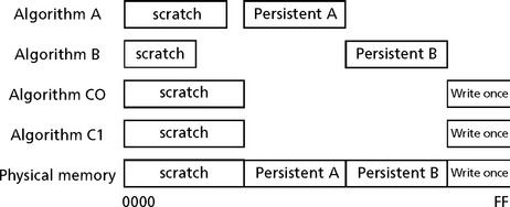
All algorithm scratch memory can be “overlaid” on the same physical memory.
Without the distinction between scratch and persistent memory, it would be necessary to strictly partition memory among algorithms, making the total memory requirement the sum of all algorithms’ memory requirements. On the other hand, by making the distinction, the total memory requirement for a collection of algorithms is the sum of each algorithm’s distinct persistent memory, plus any shared write-once persistent memory, plus the maximum scratch memory requirement of any of these algorithms.
Guideline 1
Algorithms should minimize their persistent data memory requirements in favor of scratch memory. In addition to the types of memory described above, there are often several memory spaces provided by a DSP to algorithms.
• Dual-access memory (DARAM) is on-chip memory that allows two simultaneous accesses in a single instruction cycle.
• Single-access memory (SARAM) is on-chip memory that allows only a single access per instruction cycle.
• External memory is memory that is external to the DSP and may require more than zero wait states per access.
These memory spaces are often treated very differently by algorithm implementations; in order to optimize performance, frequently accessed data is placed in on-chip memory, for example. The scratch vs. persistent attribute of a block of memory is independent of the memory space. Thus, there are six distinct memory classes; scratch and persistent for each of the three memory spaces described above.
Algorithm vs. application
Other than a memory block’s size, alignment, and memory space, three independent questions must be answered before a client can properly manage a block of an algorithm’s data memory.
• Is the block of memory treated as scratch or persistent by the algorithm?
• Is the block of memory shared by more than one algorithm?
• Do the algorithms that share the block preempt one another?
The first question is determined by the implementation of the algorithm; the algorithm must be written with assumptions about the contents of certain memory buffers. There is significant benefit to distinguish between scratch memory and persistent memory, but it is up to the algorithm implementation to trade the benefits of increasing scratch, and decreasing persistent memory against the potential performance overhead incurred by re-computing intermediate results.
The second two questions regarding sharing and preemption, can only be answered by the client of a DSP algorithm. The client decides whether preemption is required for the system and the client allocates all memory. Thus, only the client knows whether memory is shared among algorithms. Some frameworks, for example, never share any allocated memory among algorithms whereas others always share scratch memory.
There is a special type of persistent memory managed by clients of algorithms that is worth distinguishing: shadow memory is unshared persistent memory that is used to shadow or save the contents of shared registers and memory in a system. Shadow memory is not used by algorithms; it is used by their clients to save the memory regions shared by various algorithms.
Figure F.4 illustrates the relationship between the various types of memory.

Program memory
Like the data memory requirements described in the previous section, it is important that all DSP algorithms are fully relocatable; i.e., there should never be any assumption about the specific placement of an algorithm at a particular address. Alignment on a specified page size should be permitted, however.
Rule 4
All algorithm code must be fully relocatable. That is, there can be no hard coded program memory locations. As with the data memory requirements, this rule only requires that code be relocated via a linker. For example, it is not necessary to always use PC-relative branches. This requirement allows the system developer to optimally allocate program space to the various algorithms in the system. Algorithm modules sometimes require initialization code that must be executed prior to any other algorithm method being used by a client. Often this code is only run once during the lifetime of an application. This code is effectively “dead” once it has been run at startup. The space allocated for this code can be reused in many systems by placing the “run-once” code in data memory and using the data memory during algorithm operation. A similar situation occurs in “finalization” code. Debug versions of algorithms, for example, sometimes implement functions that, when called when a system exits, can provide valuable debug information; e.g., the existence of objects or objects that have not been properly deleted. Since many systems are designed to never exit (i.e., exit by poweroff), finalization code should be placed in a separate object module. This allows the system integrator to avoid including code that can never be executed.
Guideline 2
Each initialization and finalization function should be defined in a separate object module; these modules must not contain any other code. In some cases, it is awkward to place each function in a separate file. Doing so may require making some identifiers globally visible or require significant changes to an existing code base. Some DSP C compilers support a pragma directive that allows you to place specified functions in distinct COFF output sections. This pragma directive may be used in lieu of placing functions in separate files. The table below summarizes recommended section names and their purpose.
| Section | Name | Purpose |
| Text:init | Run once | Initialization code |
| Text:exit | Run once | Finalization code |
| Text:create | Run time | Object creation |
| Text:delete | Run time | Object deletion |
ROM-ability
There are several addressing modes used by algorithms to access data memory. Sometimes the data is referenced by a pointer to a buffer passed to the algorithm, and sometimes an algorithm simply references global variables directly. When an algorithm references global data directly, the instruction that operates on the data often contains the address of the data (rather than an offset from a data page register, for example). Thus, this code cannot be placed in ROM without also requiring that the referenced data be placed in a fixed location in a system. If a module has configuration parameters that result in variable length data structures and these structures are directly referenced, such code is not considered ROM-able; the offsets in the code are fixed and the relative positions of the data references may change. Alternatively, algorithm code can be structured to always use offsets from a data page for all fixed length references and place a pointer in this page to any variable length structures. In this case, it is possible to configure and locate the data anywhere in the system, provided the data page is appropriately set.
Rule 5
Algorithms must characterize their ROM-ability; i.e., state whether or not they are ROM-able. Obviously, self-modifying code is not ROM-able. We do not require that no algorithm employ self-modifying code; we only require documentation of the ROM-ability of an algorithm. It is also worth pointing out that if self-modifying code is used, it must be done “atomically,” i.e., with all interrupts disabled; otherwise this code would fail to be reentrant.
Use of peripherals
To ensure the interoperability of DSP algorithms, it is important that algorithms never directly access any peripheral device.
Rule 6
Algorithms must never directly access any peripheral device. This includes but is not limited to on-chip DMAs, timers, I/O devices, and cache control registers. In order for an algorithm to be framework-independent, it is important that no algorithm directly calls any device interface to read or write data. All data produced or consumed by an algorithm must be explicitly passed to the algorithm by the client. For example, no algorithm should call a device-independent I/O library function to get data; this is the responsibility of the client or framework.
DSP Algorithm Component Model
This section should describe in detail, the rules and guidelines that apply to all algorithms on all DSP architectures regardless of application area.
These rules and guidelines enable many of the benefits normally associated with object-oriented and component-based programming but with little or no overhead. More importantly, these guidelines are necessary to enable two different algorithms to be integrated into a single application without modifying the source code of the algorithms. The rules include naming conventions to prevent duplicate external name conflicts, a uniform method for initializing algorithms, and specification of a uniform data memory management mechanism.
There is a lot that can be written concerning this level of the standard, and it makes sense at this point to reference the details of a particular Algorithm Component Model. Please reference the following URL for the details of one DSP Algorithm Component Model
http://focus.ti.com/lit/ug/spru352e/spru352e.pdf
A summary of the rules from this standard is listed at the end of this appendix.
DSP Algorithm Performance Characterization
In this section, we need to define the performance information that should be provided by algorithm components to enable system integrators to assemble combinations of algorithms into reliable products.
The only resources consumed by most DSP algorithms are MIPS and memory. All I/O, peripheral control, device management, and scheduling should be managed by the application—not the algorithm. Thus, we need to characterize code and data memory requirements and worst-case execution time. There is one important addition, however. It is possible for an algorithm to inadvertently disrupt the scheduling of threads in a system by disabling interrupts for extended periods. Since it is not possible for a scheduler to get control of the CPU while interrupts are disabled, it is important that algorithms minimize the duration of these periods and document the worst-case duration. It is important to realize that, due to the pipeline of modern DSPs, there are many situations where interrupts are implicitly disabled; e.g., in some zero-overhead loops. Thus, even if an algorithm does not explicitly disable interrupts, it may cause interrupts to be disabled for extended periods. The main areas to define and document are:
Data memory
All data memory for an algorithm falls into one of three categories:
• Heap memory – data memory that is potentially (re)allocated at run-time;
Heap memory is bulk memory that is used by a function to perform its computations. From the function’s point of view, the location and contents of this memory may persist across functions calls, may be (re)allocated at run-time, and different buffers may be in physically distinct memories. Stack memory, on the other hand, is scratch memory whose location may vary between consecutive function calls, is allocated and freed at run-time, and is managed using a LIFO (Last In First Out) allocation policy. Finally, static data is any data that is allocated at design-time (i.e., program-build time) and whose location is fixed during run-time. In this section, we should define performance metrics that describe an algorithm’s data memory requirements.
Program memory
Algorithm code can often be partitioned into two distinct types: frequently accessed code and infrequently accessed code. Obviously, inner loops of algorithms are frequently accessed. However, like most application code, it is often the case that a few functions account for most of the MIPS required by an application.
Interrupt latency
In most DSP systems, algorithms are started by the arrival of data and the arrival of data is signaled by an interrupt. It is very important, therefore, that interrupts occur in as timely a fashion as possible. In particular, algorithms should minimize the time that interrupts are disabled. Ideally, algorithms would never disable interrupts. In some DSP architectures, however, zero overhead loops implicitly disable interrupts and, consequently, optimal algorithm efficiency often requires some interrupt latency.
Execution time
It is also important to define the execution time information that should be provided by algorithm components to enable system integrators to assemble combinations of algorithms into reliable products.
MIPS is not enough
It is important to realize that a simple MIPS calculation is far from sufficient when combining multiple algorithms. It is possible, for example, for two algorithms to be “unschedulable” even though only 84% of the available MIPS are required. In the worst case, it is possible for a set of algorithms to be unschedulable although only 70% of the available MIPS are required!
Suppose, for example, that a system consists of two tasks A and B with periods of 2 ms and 3 ms respectively (Figure F.5). Suppose that task A requires 1 ms of the CPU to complete its processing and task B also requires 1 ms of the CPU. The total percentage of the CPU required by these two tasks is approximately 83.3%; 50% for task A plus 33.3% for task B.

In this case, both task A and B meet their deadlines and we have more than 18% (1 ms every 6 ms) of the CPU idle. Suppose we now increase the amount of processing that task B must perform very slightly, say to 1.0000001 ms every 3 ms. Notice that task B will miss its first deadline because task A consumes 2 ms of the available 3 ms of task B’s period. This leaves only 1 ms for B but B needs just a bit more than 1 ms to complete its work. If we make task B higher priority than task A, task A will miss its deadline line because task B will consume more than 1 ms of task A’s 2 ms period. In this example, we have a system that has over 18% of the CPU MIPS unused but we cannot complete both task A and B within their real-time deadlines.
Moreover, the situation gets worse if you add more tasks to the system.
Liu and Layland proved that in the worst case you may have a system that is idle slightly more than 30% of the time that still can’t meet its real-time deadlines! The good news is that this worst-case situation does not occur very often in practice. The bad news is that we can’t rely on this not happening in the general situation. It is relatively easy to determine if a particular task set will meet its real-time deadlines if the period of each task is known and its CPU requirements during this period are also known. It is important to realize, however, that this determination is based on a mathematical model of the software and, as with any model, it may not correspond 100% with reality.
Moreover, the model is dependent on each component accurately characterizing its performance; if a component underestimates its CPU requirements by even 1 clock cycle, it is possible for the system to fail. Finally, designing with worst-case CPU requirements often prevents one from creating viable combinations of components. If the average case CPU requirement for a component differs significantly from its worst case, considerable CPU bandwidth may be wasted.
DSP-Specific Guidelines
DSP algorithms are often written in assembly language and, as a result, they will take full advantage of the instruction set. Unfortunately for the system integrator, this often means that multiple algorithms cannot be integrated into a single system because of incompatible assumptions about the use of specific features of the DSP (e.g., use of overflow mode, use of dedicated registers, etc.). This section should cover those guidelines that are specific to a particular DSP instruction set. These guidelines are designed to maximize the flexibility of the algorithm implementers, while at the same time ensure that multiple algorithms can be integrated into a single system. The standard should include things like;
CPU register types
The standard should include several categories of register types.
• Scratch register – These registers can be freely used by an algorithm, cannot be assumed to contain any particular value upon entry to an algorithm function, and can be left in any state after exiting a function.
• Preserve registers – These registers may be used by an algorithm, cannot be assumed to contain any particular value upon entry to an algorithm function, but must be restored upon exit from an algorithm to the value it had at entry.
• Initialized register – These registers may be used by an algorithm, contain a specified initial value upon entry to an algorithm function (as stated next to the register), and must be restored upon exit from the algorithm.
• Read-only register – These registers may be read but must not be modified by an algorithm.
In addition to the categories defined above, all registers should be further classified as being either local or global. Local registers are thread specific; i.e., every thread maintains its own copy of this register and it is active whenever this thread is running. Global registers, on the other hand, are shared by all threads in the system; if one thread changes a global register then all threads will see the change.
Use of floating-point
Referencing the float data type in an algorithm on a fixed-point DSP causes a large floating-point support library to be included in any application that uses the algorithm.
Endian byte ordering
DSP families support both big and little endian data formats. This support takes the form of “boot time” configuration. The DSP may be configured at boot time to access memory either as big endian or little endian and this setting remains fixed for the lifetime of the application.
The choice of which data format to use is often decided based on the presence of other processors in the system; the data format of the other processors (which may not be configurable) determines the setting of the DSP data format. Thus, it is not possible to simply choose a single data format for DSP algorithms.
Data models
DSP C compilers support a variety of data models; one small model and multiple large model modes. Fortunately, it is relatively easy to mix the various data memory models in a single application. Programs will achieve optimal performance using small model compilation. This model limits, however, the total size of the directly accessed data in an application to 32K bytes (in the worst case). Since algorithms are intended for use in very large applications, all data references should be far references.
Program model
DSP algorithms must never assume placement in on-chip program memory; i.e., they must properly operate with program memory operated in cache mode. In addition, no algorithm may ever directly manipulate the cache control registers. It is important to realize that compliant algorithms may be placed in on-chip program memory by the system developer. The rule above simply states that algorithms must not require placement in on-chip memory.
Register conventions
There must also be rules and guidelines that apply to the use of DSP on-chip registers. There are several different register types. Only those registers that are specifically defined with a programming model are allowed to be accessed. The list below is an example of a register set that must be defined with a programming model (register use rules):
• Address mode register Init (local)
• General-purpose Scratch (local)
• General-purpose Preserve (local)
• Frame Pointer Preserve (local)
• Data Page pointer Preserve (local)
• Stack Pointer Preserve (local)
• Control and Status Register Preserve
• Interrupt clear register Not accessible (global)
• Interrupt enable register Read-only (global)
• Interrupt flag register Read-only (global)
• Interrupt return pointer Scratch (global)
• Interrupt set register Not accessible (global)
• Interrupt service table pointer Read-only (global)
Status register
DSPs, like other embedded processors, contain status registers. This status register is further divided into several distinct fields. Although each field is often thought of as a separate register, it is not possible to access these fields individually. For example, in order to set one field it may be necessary to set all fields in the same status register. Therefore, it is necessary to treat the status registers with special care; if any field of a status register is of type Preserve or Read-only, the entire register must be treated as a Preserve register, for example.
Interrupt latency
Although there are no additional rules for DSP algorithms that deal with interrupt latency, it may be necessary to understand some important architectural impacts that DSPs have with respect to algorithmic execution. For example, on some DSPs, all instructions in the delay slots of branches are noninterruptible; i.e., once fetched, interrupts are blocked until the branch completes. Since these delay slots may contain other branch instructions, care must be taken to avoid long chains of noninterruptible instructions. In particular, tightly coded loops often result in unacceptably long noninterruptible sequences. Note that the C compiler has options to limit the duration of loops. Even if this option is used, you must be careful to limit the length of loops whose length is not a simple constant.
Use of the DMA Resource for Algorithm Development
The direct memory access (DMA) controller performs asynchronously scheduled data transfers in the background while the CPU continues to execute instructions. A good DSP algorithm standard should include rules and guidelines for creating compliant DSP algorithms that utilize the DMA resources.
The fact is that some algorithms require some means of moving data in the background of CPU operations. This is particularly important for algorithms that process and move large blocks of data; for example, imaging and video algorithms. The DMA is designed for this exact purpose and algorithms need to gain access to this resource for performance reasons.
A DSP algorithm standard should outline a model to facilitate the use of the DMA resources for these DSP algorithms.
A DSP algorithm standard should look upon algorithms as pure “data transducers.” They are, among other things, not allowed to perform any operations that can affect scheduling or memory management. All these operations must be controlled by the framework to ensure easy integration of algorithms, possibly from different vendors. In general, the framework must be in command of managing the system resources, including the DMA resource.
Algorithms cannot access the DMA registers directly, nor can they be written to work with a particular physical DMA channel only. The framework must have the freedom to assign any available channel, and possibly share DMA channels, when granting an algorithm a DMA resource.
Requirements for the use of the DMA resource
Below is a list of requirements for DMA usage in DSP algorithms. These requirements will help to clarify the intent of the stated rules and guidelines in this chapter.
1. All physical DMA resources must be owned and managed by the framework.
2. Algorithms must access the DMA resource through a handle representing a logical DMA channel abstraction. These handles are granted to the algorithm by the framework using a standard interface.
3. A mechanism must be provided so that algorithms can ensure completion of data transfer(s).
4. The DMA scheme must work within a preemptive environment.
5. It must be possible for an algorithm to request multiframe data transfers (two-dimensional data transfers).
6. The framework must be able to obtain the worst-case DMA resource requirements at algorithm initialization time.
7. The DMA scheme must be flexible enough to fit within static and dynamic systems, and systems with a mix of static and dynamic features.
8. All DMA operations must complete prior to return to caller. The algorithm must synchronize all DMA operations before return to the caller from a framework-callable operation.
9. It must be possible for several algorithms to share a physical DMA channel.
For details of an existing algorithm standard that details the use of the DMA in algorithm develop, see the previously mentioned URL.
Rules and Guidelines for DSP Algorithm Development
This section will summarize the general rules, DSP specific rules, performance characterization rules, and DMA use rules for an existing DSP algorithm standard as well as some guidelines. This can be tailored accordingly.
General Rules
Rule 1 All algorithms must follow the run-time conventions imposed by the implementation of the C programming language.
Rule 2 All algorithms must be reentrant within a preemptive environment (including time-sliced preemption).
Rule 3 All algorithm data references must be fully relocatable (subject to alignment requirements). That is, there must be no “hard coded” data memory locations.
Rule 4 All algorithm code must be fully relocatable. That is, there can be no hard coded program memory locations
Rule 5 Algorithms must characterize their ROM-ability; i.e., state whether they are ROM-able or not.
Rule 6 Algorithms must never directly access any peripheral device. This includes but is not limited to on-chip DMAs, timers, I/O devices, and cache control registers.
Note, however, algorithms can utilize the DMA resource by implementing the appropriate interface.
Rule 7 All header files must support multiple inclusions within a single source file.
Rule 8 All external definitions must be either API identifiers or API and vendor prefixed.
Rule 9 All undefined references must refer either to the operations specified in the appropriate C runtime support library functions or the appropriate library functions.
Rule 10 All modules must follow compliant naming conventions for those external declarations disclosed to clients of those algorithms.
Rule 11 All modules must supply an initialization and finalization method.
Rule 12 All algorithms must implement the appropriately defined interfaces.
Rule 13 Each of the methods implemented by an algorithm must be independently relocatable.
Rule 14 All abstract algorithm interfaces must derive from a standard interface definition.
Rule 15 Each DSP algorithm must be packaged in an archive which has a name that follows a uniform naming convention.
Rule 16 Each DSP algorithm header must follow a uniform naming convention.
Rule 17 Different versions of a DSP algorithm from the same vendor must follow a uniform naming convention.
Rule 18 If a module’s header includes definitions specific to a “debug” variant, it must use a common symbol to select the appropriate definitions; the symbol is defined for debug compilations and only for debug compilations.
Examples of DSP Specific Rules
Rule 25 All DSP algorithms must be supplied in little-endian format.
Rule 26 All DSP algorithms must access all static and global data as far data.
Rule 27 DSP algorithms must never assume placement in on-chip program memory; i.e., they must properly operate with program memory operated in cache mode.
Rule 28 On processors that support large program model compilation, all function accesses to independently relocatable object modules must be far references. For example, intersection function references within algorithm and external function references to other DSP modules must be far on the specific DSP type; i.e., the calling function must push both the XPC and the current PC.
Rule 29 On processors that support large program model compilation, all independently relocatable object module functions must be declared as far functions; for example, on the specific DSP, callers must push both the XPC and the current PC and the algorithm functions must perform a far return.
Rule 30 On processors that support an extended program address space (paged memory), the code size of any independently relocatable object module should never exceed the code space available on a page when overlays are enabled.
Rule 31 All DSP algorithms must document the content of the stack configuration register that they follow.
Rule 32 All DSP algorithms must access all static and global data as far data; also the algorithms should be instantiable in a large memory model.
Rule 33 DSP algorithms must never assume placement in on-chip program memory; i.e., they must properly operate with program memory operated in instruction cache mode.
Rule 34 All DSP algorithms that access data by B-bus must document: the instance number of the IALG_MemRec structure that is accessed by the B-bus (heapdata), and the data-section name that is accessed by the B-bus (static-data).
Rule 35 All DSP algorithms must access all static and global data as far data; also, the algorithm should be instantiable in a large memory model.
Performance Characterization Rule
Rule 19 All algorithms must characterize their worst-case heap data memory requirements (including alignment).
Rule 20 All algorithms must characterize their worst-case stack space memory requirements (including alignment).
Rule 21 Algorithms must characterize their static data memory requirements.
Rule 22 All algorithms must characterize their program memory requirements.
Rule 23 All algorithms must characterize their worst-case interrupt latency for every operation.
Rule 24 All algorithms must characterize the typical period and worst-case execution time for each operation.
DMA Rules
DMA Rule 1 All data transfer must be completed before return to caller.
DMA Rule 2 All algorithms using the DMA resource must implement a standard interface.
DMA Rule 3 Each of the DMA methods implemented by an algorithm must be independently relocateable.
DMA Rule 4 All algorithms must state the maximum number of concurrent DMA transfers for each logical channel.
DMA Rule 5 All algorithms must characterize the average and maximum size of the data transfers per logical channel for each operation. Also, all algorithms must characterize the average and maximum frequency of data transfers per logical channel for each operation.
DMA Rule 6 For certain DSP (like the C6x) algorithms must not issue any CPU read/writes to buffers in external memory that are involved in DMA transfers. This also applies to the input buffers passed to the algorithm through its algorithm interface.
DMA Rule 7 If a DSP algorithm has implemented the DMA interface, all input and output buffers residing in external memory and passed to this algorithm through its function calls, should be allocated on a cache line boundary and be a multiple of the cache line length in size. The application must also clean the cache entries for these buffers before passing them to the algorithm.
DMA Rule 8 When appropriate, all buffers residing in external memory involved in a DMA transfer should be allocated on a cache line boundary and be a multiple of the cache line length in size.
DMA Rule 9 When appropriate, algorithms should not use stack allocated buffers as the source or destination of any DMA transfer.
DMA Rule 10 When appropriate, algorithms must request all data buffers in external memory with 32-bit alignment and sizes in multiples of 4 (bytes).
DMA Rule 11 When appropriate, algorithms must use the same data types, access modes and DMA transfer settings when reading from or writing to data stored in external memory, or in application-passed data buffers.
General Guidelines
Guideline 1 Algorithms should minimize their persistent data memory requirements in favor of scratch memory.
Guideline 2 Each initialization and finalization function should be defined in a separate object module; these modules must not contain any other code.
Guideline 3 All modules that support object creation should support design-time object creation.
Guideline 4 All modules that support object creation should support run-time object creation.
Guideline 5 Algorithms should keep stack size requirements to a minimum.
Guideline 6 Algorithms should minimize their static memory requirements.
Guideline 7 Algorithms should never have any scratch static memory.
Guideline 8 Algorithm code should be partitioned into distinct sections and each section should be characterized by the average number of instructions executed per input sample.
Guideline 9 Interrupt latency should never exceed 10 s. (or other appropriate measure)
Guideline 10 Algorithms should avoid the use of global registers.
Guideline 11 Algorithms should avoid the use of the float data type.
Guideline 12 When appropriate, all algorithms should be supplied in both little- and big-endian formats.
Guideline 13 On processors that support large program model compilations, a version of the algorithm should be supplied that accesses all core run-time support functions as near functions and all algorithms as far functions (mixed model).
Guideline 14 When appropriate, all algorithms should not assume any specific stack configuration and should work under all the three stack modes.
DMA Guidelines
Guideline 1 The data transfer should complete before the CPU operations executing in Parallel.
Guideline 2 All algorithms should minimize channel (re)configuration overhead by requesting a dedicated logical DMA channel for each distinct type of DMA transfer it issues.
Guideline 3 To ensure correctness, All DSP algorithms that use DMA need to be supplied with the internal memory they request from the client application.
Guideline 4 To facilitate high performance, DSP algorithms should request DMA transfers with source and destinations aligned on 32-bit byte addresses (when appropriate).
Guideline 5 DSP algorithms should minimize channel configuration overhead by requesting a separate logical channel for each different transfer type.
Glossary
Abstract Interface An interface defined by a C header whose functions are specified by a structure of function pointers. By convention these interface headers begin with the letter ‘i’ and the interface name begins with ‘I’. Such an interface is “abstract” because, in general, many modules in a system implement the same abstract interface; i.e., the interface defines abstract operations supported by many modules.
Algorithm Technically, an algorithm is a sequence of operations, each chosen from a finite set of well-defined operations (e.g. computer instructions), that halts in a finite time, and computes a mathematical function. In the context of this specification, however, we allow algorithms to employ heuristics and do not require that they always produce a correct answer.
API Acronym for Application Programming Interface i.e., a specific set of constants, types, variables, and functions used to programmatically interact with a piece of software
Asynchronous System Calls Most system calls block (or “suspend”) the calling thread until they complete, and continue its execution immediately following the call. Some systems also provide asynchronous (or nonblocking) forms of these calls; the kernel notifies the caller through some kind of out-of-band method when such a system call has completed. Asynchronous system calls are generally much harder for the programmer to deal with than blocking calls. This complexity is often outweighed by the performance benefits for real-time compute intensive applications.
Client The term client is often used to denote any piece of software that uses a function, module, or interface; for example, if the function a() calls the function b(), a() is a client of b(). Similarly, if an application App uses module MOD, App is a client of MOD.
COFF Common Output File Format. The file format of the files produced by the TI compiler, assembler, and linker.
Concrete Interface An interface defined by a C header whose functions are implemented by a single module within a system. This is in contrast to an abstract interface where multiple modules in a system may implement the same abstract interface. The header for every module defines a concrete interface.
Context Switch A context switch is the action of switching a CPU between one thread and another (or transferring control between them). This may involve crossing one or more protection boundaries.
Critical Section A critical section of code is one in which data that may be accessed by other threads are inconsistent. At a higher level, a critical section can be viewed as a section of code in which a guarantee you make to other threads about the state of some data may not be true. If other threads can access these data during a critical section, your program may not behave correctly. This may cause it to crash, lock up, produce incorrect results, or do just about any other unpleasant thing you care to imagine. Other threads are generally denied access to inconsistent data during a critical section (usually through use of locks). If some of your critical sections are too long, however, it may result in your code performing poorly.
Endian Refers to which bytes are most significant in multibyte data types. In big-endian architectures, the leftmost bytes (those with a lower address) are most significant. In little-endian architectures, the rightmost bytes are most significant. HP, IBM, Motorola 68000, and SPARC systems store multibyte values in big-endian order, while Intel 80x86, DEC VAX, and DEC Alpha systems store them in little-endian order. Internet standard byte ordering is also big-endian. The TMS320C6000 is bi-endian because it supports both systems.
Frame Algorithms often process multiple samples of data at a time. This set of samples is sometimes referred to as a frame. In addition to improving performance, some algorithms require specific minimum frame sizes to properly operate.
Framework A framework is that part of an application that has been designed to remain invariant while selected software components are added, removed, or modified. Very general frameworks are sometimes described as application specific operating systems.
Instance The specific data allocated in an application that defines a particular object.
Interface A set of related functions, types, constants, and variables. An interface is often specified via a C header file.
Interrupt Latency The maximum time between when an interrupt occurs and its corresponding Interrupt Service Routine (ISR) starts executing.
Glossary of Terms
Interrupt Service Routine (ISR) An ISR is a function called in response to an interrupt detected by a CPU.
Method The term method is a synonym for a function that can be applied to an object defined by an interface.
Module A module is an implementation of one (or more) interfaces. In addition, all modules follow certain design elements that are common to all standard-compliant software components. Roughly speaking, a module is a C language implementation of a C++ class. Since a module is an implementation of an interface, it may consist of many distinct object files.
Multithreading Multithreading is the management of multiple concurrent uses of the same program. Most operating systems and modern computer languages also support multithreading.
Preemptive A property of a scheduler that allows one task to asynchronously interrupt the execution of the currently executing task and switch to another task; the interrupted task is not required to call any scheduler functions to enable the switch.
Protection Boundary A protection boundary protects one software subsystem on a computer from another, in such a way that only data that is explicitly shared across such a boundary is accessible to the entities on both sides. In general, all code within a protection boundary will have access to all data within that boundary. The canonical example of a protection boundary on most modern systems is that between processes and the kernel. The kernel is protected from processes, so that they can only examine or change its internal state in certain strictly defined ways. Protection boundaries also exist between individual processes on most modern systems. This prevents one buggy or malicious process from wreaking havoc on others. Why are protection boundaries interesting? Because transferring control across them is often expensive; it takes a lot of time and work. Most DSPs have no support for protection boundaries.
Reentrant Pertaining to a program or a part of a program in its executable version, that may be entered repeatedly, or may be entered before previous executions have been completed, and each execution of such a program is independent of all other executions.
Run to Completion A thread execution model in which all threads run to completion without ever synchronously suspending execution. Note that this attribute is completely independent of whether threads are preemptively scheduled. Run to completion threads may be preempt on another (e.g., ISRs) and nonpreemptive systems may allow threads to synchronously suspend
Glossary of Terms
D-4 execution Note that only one run-time stack is required for all run to completion threads in a system.
Scheduling The process of deciding what thread should execute next on a particular CPU. It is usually also taken as involving the context switch to that thread.
Scheduling Latency The maximum time that a “ready” thread can be delayed by a lower priority thread.
Scratch Memory Memory that can be overwritten without loss; i.e., prior contents need not be saved and restored after each use.
Scratch Register A register that can be overwritten without loss; i.e., prior contents need not be saved and restored after each use.
Thread The program state managed by the operating system that defines a logically independent sequence of program instructions. This state may be as little as the Program Counter (PC) value but often includes a large portion of the CPU’s register set.
This appendix lists sources for additional information.
Dialogic. Media Stream Processing Unit; Developer’s Guide. September 1998. 05-1221-001-01
ISO/IEC JTC1/SC22 N 2388 dated January 1997, Request for SC22 Working Groups to Review DIS 2382-07.
Mwave Developer’s Toolkit. DSP Toolkit User’s Guide. 1993.
Liu, C.L., Layland, J.W. “Scheduling Algorithms for Multi-Programming in a Hard Real-Time Environment,”. JACM. January 1973;20(1):40–61.
Hard Real-Time Environment,” JACM 20, 1, (January 1973): 40-61.
Massey, Tim, Iyer, Ramesh. DSP Solutions for Telephony and Data/Facimile Modems. SPRA073. 1997.
Texas Instruments. TMS320C54x Optimizing C Compiler User’s Guide. SPRU103C. 1998.
Texas Instruments. TMS320C6x Optimizing C Compiler User’s Guide. SPRU187C. 1998.
Texas Instruments. TMS320C62xx CPU and Instruction Set. SPRU189B. 1997.
Texas Instruments. TMS320C55x Optimizing C/C++ Compiler User’s Guide. SPRU281. 2001.
Texas Instruments. TMS320C2x/C2xx/C5x Optimizing C Compiler User’s Guide. SPRU024. 1999.
Texas Instruments. TMS320C28x Optimizing C/C++ Compiler User’s Guide. SPRU514. 2001.