7
One Qubit
Anyone who is not shocked by
quantum theory has not understood it.
A quantum bit, or qubit, is the fundamental information unit of quantum computing. In this chapter, I give a mathematical definition of a qubit based on the foundational material in the first part of this book. Together we examine the operations you can perform on a single qubit from both mathematical and computational perspectives.
Despite a single qubit living in a seemingly strange two-dimensional complex Hilbert space, we can visualize it, its superposition, and its behavior by projecting onto the surface of a sphere in R3.
All vector spaces considered in this chapter are over C, the field of complex numbers introduced in section 3.9 . All bases are orthonormal unless otherwise specified.
Topics covered in this chapter
7.2 Bras and kets
7.3 The complex math and physics of a single qubit
7.3.1 Quantum state representation
7.3.2 Unitary matrices mapping to standard form
7.3.3 The density matrix
7.3.4 Observables and expectation
7.4 A non-linear projection
7.5 The Bloch sphere
7.6 Professor Hadamard, meet Professor Pauli
7.6.1 The quantum X gate
7.6.2 The quantum Z gate
7.6.3 The quantum Y gate
7.6.4 The quantum ID gate
7.6.5 The quantum H gate
7.6.6 The quantum Rϕz gates
7.6.7 The quantum S gate
7.6.8 The quantum S† gate
7.6.9 The quantum T gate
7.6.10 The quantum T† gate
7.6.11 The quantum Rϕx and Rϕy gates
7.6.12 The quantum √NOT gate
7.6.13 The quantum |0> RESET operation
7.7 Gates and unitary matrices
7.8 Summary
7.1 Introducing quantum bits
If you have seen descriptions of qubits elsewhere, you may have read something like ‘‘a qubit implements a two-state quantum mechanical system and is the quantum analog of a classical bit.’’ A bit, as we saw in section 2.1, also has two states, those being 0 and 1.
Those other discussions then usually include one or more of the following: light switches, spinning electrons, polarized light, and rotating coins or donuts. I don’t spend my days thinking about electrons but I do like sunglasses and donuts. These approaches all have merit and are the basis for teasing apart the difference between the quantum and classical situations. The electron and polarized light examples do depict quantum systems.
Otherwise, analogies tend to be imperfect and eventually may lead you into corners where their behavior and your understanding are not consistent with the real situation. It’s for this reason we developed the essential mathematics and insight to reason accurately about what happens in quantum computing.
Let’s begin by thinking about a classical bit and a quantum bit.

On the left, we have the classical situation where a bit can only take on the values 0 and 1. More precisely, a bit can be in one of those states and only those. You can look at the bit at any time and, assuming nothing has happened to change the state, it stays in that state.
For the quantum situation on the right, we change the notation slightly. The qubit always becomes the state |0⟩ or |1⟩ when we read information from it by a process called measurement. However, it is possible to move it to an infinite number of other states and change from one of them to another while we are computing with the qubit before measurement.
Measurement says ‘‘ok, I’m going to peek at the qubit now’’ and the result is always a 0 or 1 once you do so. We can then read that out as a bit value of 0 or 1, respectively.
Yes, this is weird. This is quantum mechanics and it has amazed, and befuddled, and surprised, and delighted people for close to one hundred years. Quantum computing is based on and takes advantage of this behavior.
Continuing with the right side, we represent all the states the qubit could be in as points on the unit sphere. |0⟩ is at the north pole, and |1⟩ is at the south. Remember: points on the sphere equal quantum states. In the next section I define more precisely what we mean when we write |0⟩ and |1⟩.
I need to state and then clarify something about superposition. Mathematically, the qubit is always in superposition because its state can be at the poles |0⟩ or |1⟩ or any point in between. However, by slight abuse of terminology, people typically mean the state is in superposition when it is not |0⟩ or |1⟩. If the state is not one of the poles we are speaking about a non-trivial superposition. To ‘‘move into superposition’’ usually means the state is moved to a point on the equator.
A quantum algorithm uses several qubits which together constitute a quantum register. From the viewpoint of a single qubit, its activity looks like
- I, the qubit, am in initial state |0⟩.
- I get moved into a standard superposition. Don’t peek!
- Steps in the algorithm apply zero or more reversible operations to me.
- I get measured and always become |0⟩ or |1⟩.
- When these get read out for classical use, they are converted to 0 or 1.
It’s what happens in steps 2 and 3 that make quantum computing interesting. For the unit sphere, which is called the Bloch sphere in quantum computing, step 2 means I get moved to a designated point/state on the equator. Step 3 translates to getting moved to other points/states. This movement is a result of what the algorithm is doing and causing to happen.
The final two steps are like telling the qubit ‘‘look, you can’t stay somewhere in superposition forever. You need to decide whether you will be 0 or 1. This is not optional.’’ Where it is in superposition, in what state on the sphere, determines the relative probabilities of the qubit ultimately yielding a classical bit value of 0 or 1.
If the state lies on the equator, then with perfect randomness it will end up being 0 half of the time and 1 half of the time.
Though the Bloch sphere is a convenient and visual representation, the linear algebraic description of a qubit is more fundamental, in my opinion. We go back and forth between them when one or the other makes it easier to understand some aspect of quantum computing.
Moving from the sphere back to linear algebra, compare these two statements:
- The variable q can have either the vector value v or w, and they are an orthonormal basis.
- The variable q can be any linear combination a v + b w. If a and b are non-zero the linear combination is non-trivial.
The second seems much more powerful than the first. When a = 1 and b = 0 we get v. Reversing these assignments gives us w. The second statement appears to reduce to the first when we make these choices. Alternatively, the first is extended by the second.
We explore and return to this statement throughout the rest of this chapter:
A qubit—a quantum bit—is the fundamental unit of quantum information. At any given time, it is in a superposition state represented by a linear combination of vectors |0⟩ and |1⟩ in C2:
If necessary, we can convert (‘‘read out’’) |0⟩ and |1⟩ to classical bit values of 0 and 1.
|0⟩ and |1⟩ are defined in the next section.
The word ‘‘collapse’’ comes from the physical interpretation of a quantum system where measurement causes a superposition to move to one of two choices. We examine what it is that is collapsing when we look at the quantum description of the polarization of photons in section 11.3 .
A qubit by itself is not very interesting, despite all the mathematical formalism. Algorithms need to produce results and those results should translate to something meaningful. A qubit really does eventually produce only a single classical 0 or 1 when measured and read, and so we need many more of them to represent useful information.
Quantum algorithms are interesting because of the ways multiple qubits interact when they are in their pre-measured states, when we can use the full power of using linear algebra in C2. Entanglement is the situation where two or more qubits are so tightly correlated that we cannot learn something about one without learning about the other(s).
7.2 Bras and kets
When we previously looked at vector notation in section 5.4.2 , we saw several forms like

We now add two more which were invented by Paul Dirac, an English theoretical physicist, for use in quantum mechanics. They simplify many of the expressions we use in quantum computing.
Given a vector v = (v1, v2, …, vn), we denote by ⟨v|, pronounced ‘‘bra-v’’, the row vector
When n = m, the bra-ket ⟨v | w⟩ = ⟨v| |w⟩ = (⟨v|) (|w⟩) is the usual inner product.
To avoid notational overload, I continue to put vector names in bold case like v when I use them in isolation, but will drop the bold in the bra or ket forms. They already make it clear that a vector is involved.
To learn more
How does mathematical notation get invented? As mathematicians work with concepts, they need a concise way of conveying what they mean. Good notation can make a statement or a proof much clearer and more insightful to the reader. Over time, the symbols and expressions that prove to be most useful win out while the others fade away into the archives. In the case of Dirac’s bra-ket notation, it has become ubiquitous across quantum mechanics and now quantum computing. [5, Section 1.6] [6, Section 6.2]
Example
If v = (3, −i) and w = (2 + i, 4) then
Just as we early on used n for a generic number in N or z for a number in C, |ψ⟩ is a general purpose labeled ket. The Greek letter ψ is ‘‘psi.’’
|0⟩ is (1, 0) and |1⟩ is (0, 1) in the standard basis e1 and e2. |0⟩ and |1⟩ are an orthonormal basis for C2. Remember, vectors exist independently of their representation in a given basis, so what we are really saying is:
|0⟩ is the vector in C2 that has coordinates (1, 0) when we
happen to be using the basis e1 and e2. |1⟩ has coordinates (0, 1) in this basis.
|0⟩ and |1⟩ are frequently called the computational basis.
In the same way ![]() and
and ![]() in the standard basis. Like |0⟩ and |1⟩, these are an orthonormal basis for C2.
in the standard basis. Like |0⟩ and |1⟩, these are an orthonormal basis for C2.
To remember which is |0⟩ and which is |1⟩, look at the second coordinate. For |+⟩ and |−⟩, look at the sign of the second coordinate.
Question 7.2.1
What are the coordinates for |0⟩ in the basis ![]() and
and ![]() ? What are the coordinates for |1⟩?
? What are the coordinates for |1⟩?
This diagram may help but does it make a difference that it is drawn in R2 instead of C2?
Though we use the notation |0⟩ and |1⟩, they are not equal to the numbers 0 and 1! I show a connection later when we discuss measuring the state of a qubit, but do keep them separate in your mind. The reason I highlight this is because, as a basis, any vector in C2 can be written as a linear combination
Just as we saw that a 1 by n matrix or a row vector defines a linear form, so does a bra when combined with a ket. For a vector a = (a1, a2, …, an),
For a bra ⟨v|, what does ⟨v| L mean? If A is again a matrix for L, then ⟨v| L is ⟨v| A and we do the matrix multiplication between the row vector and the matrix.
These all have the nice property that we can slide L and A from the bra to the ket and back:
| ⟨v| L × |w⟩ | = (⟨v| L) |w⟩ = ⟨v| (L |w⟩) = ⟨v| × L |w⟩ |
| ⟨v| A × |w⟩ | = (⟨v| A) |w⟩ = ⟨v| (A |w⟩) = ⟨v| × A |w⟩ |
Let V be an n-dimensional vector space and let |e1⟩ to |en⟩ be the standard basis e1, …, e2 in ket form. If A is an n by n square matrix then the (i, j)-th entry of A is Ai, j = ⟨ei | A | ej⟩.
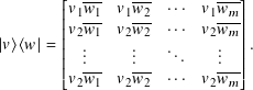
|ei⟩⟨ej| is an n by n square matrix with a 1 in the (i, j)-th position and 0 elsewhere.
The sum of the n2 matrices |ei⟩ Ai, j ⟨ej| is A.
Define matrices
| P(i) | = |ei⟩⟨ei| |
| P(i, j) | = P(i) + P(j) |
| P(i, j, k) | = P(i) + P(j) + P(k) for i ≠ j ≠ k ≠ i. |
Question 7.2.2
Show that
A Hermitian matrix A is a projector or a projection matrix if A2 = A. The rank of the projector is the dimension of its image vector space. P(i) has rank 1, P(i, j) has rank 2, and so on. P(1, …, n) = In.
Why did I bother introducing this new notation? First, it’s what scientists and practitioners in quantum mechanics and quantum computing use, and you have to know their language. Second, while it now only seems like a modest improvement over the vector and linear transformation notation we developed in chapter 5, it dramatically simplifies expressions involving multiple qubits. It provides, I hope, greater clarity and faster understanding for you.
7.3 The complex math and physics of a single qubit
Let’s revisit our definition of a qubit from section 7.1 . This time we break it into two pieces, a mathematical part and a physical/quantum mechanical part.
Mathematics
A qubit—a quantum bit—is the fundamental unit of quantum information. At any given time, it is in a superposition state represented by a linear combination of vectors |0⟩ and |1⟩ in C2:
Physics
Through measurement, a qubit is forced to collapse irreversibly to either |0⟩ or |1⟩. The probability of its doing either is |a|2 and |b|2, respectively. a and b are called probability amplitudes.
The mathematical portion is linear algebra of a two-dimensional complex vector space. As a vector, the qubit state has length 1. Linear transformations must preserve this length and are isometries. Their matrices are unitary. Being unitary, they are invertible: moving a qubit from one state to another is always reversible.
When we built circuits that manipulated bits in section 2.4 , only one of the core gates, not, was reversible. When we build quantum circuits using qubits in chapter 9, all the gates are reversible with the exception of measurement. Mathematically, we can think of a quantum circuit as the application of unitary matrices to vectors representing qubit states.
Mathematics is elegant and beautiful in its own right but it is often only a tool used in other fields. We frequently use it to build models that allow us to reason about how things may work in the so-called ‘‘real world.’’ These models themselves are not the real world but are our best effort to formalize the relationships that seem to make things behave the way they do.
Linear algebra by itself does not say the probability amplitudes affect whether we get |0⟩ or |1⟩ when a qubit is measured. Linear algebra, complex numbers, and probability are used to represent much of quantum computing. We must use our understanding of the physical system to interpret what the elements of the mathematics mean. Mathematical formalism can only get us so far in the development of our structure: physics must give us additional relationships that bring us further.
In particular, measurement is a physical action. It causes us to drop from a superposition state involving |0⟩ and |1⟩ to one or the other. Mathematics describes the probability of either being produced but it does not force one value or another.
7.3.1 Quantum state representation
If |ψ⟩ = a |0⟩ + b |1⟩ is a quantum state, we know |ψ|2 = |a|2 + |b|2 = 1. This is the same as saying ⟨ψ | ψ⟩ = 1.
The values |a|2 and |b|2 are non-negative numbers in R that are the probabilities that |ψ⟩ will go to |0⟩ or |1⟩, respectively, when measured.
Consider the following example in which, for illustrative purposes, I have made some simplifications and taken some labeling liberties. Suppose a and b can only be real.
Let a = 1/2 and b = √3/2. Then |a|2 = |1/2|2 = 0.25 and |b|2 = |√3/2|2 = 0.75. This means that the state of the qubit has a 25% chance of collapsing to |0⟩ when measured and a 75% chance of collapsing to |1⟩.

If c is in C with |c| = 1, then
We identify two quantum states if they only differ by a multiple of a complex unit. Recall that a unit has absolute value equal to 1. Such numbers look like ei ϕ for 0 ≤ ϕ < 2π.
This has the consequence that when we say ‘‘|ψ⟩ is not changed,’’ we really mean that after doing whatever we are doing, ‘‘it is fine if we have eiϕ |ψ⟩.’’ This point is easy to miss because you expect |ψ⟩ to be literally unchanged.
Let’s re-express a and b in polar form:
There’s a whole lot of subscripting and superscripting going on there! The net is this: from the perspective of measurement and observable results,
We are left with two degrees of freedom for the state of a qubit:
- one related to the magnitudes since r1 and r2 are dependent via |r1|2 + |r2|2 = 1, and
- the relative phase ϕ2 − ϕ1.
The relative phase is significant and is important when we see interference in section 9.6, a technique used in quantum algorithms.
The state of a single qubit |ψ⟩ can be represented by
When two quantum states |ψ⟩1 and |ψ⟩2 differ only by a complex unit multiple u,
7.3.2 Unitary matrices mapping to standard form
If |ψ⟩= cos(θ/2) |0⟩ + sin(θ/2) eϕ i |1⟩ is an arbitrary quantum state where we have made the first probability amplitude real, then what does a 2 by 2 unitary matrix U look like that maps |0⟩ to |ψ⟩?

7.3.3 The density matrix
For |ψ⟩ = a |0⟩ + b |1⟩, we define the density matrix of |ψ⟩ to be
Question 7.3.1
What is det(|ψ⟩⟨ψ|)?

From this we can compute ![]() ,
, ![]() , and
, and ![]() . Up to a global phase, we have not lost anything from going from the ket to the density matrix.
. Up to a global phase, we have not lost anything from going from the ket to the density matrix.
Question 7.3.2
What can you tell about the original ket if given its density matrix
For |ψ⟩ expressed generally by r1 eϕ1 i|1⟩ |0⟩ + r2 eϕ2 i|1⟩, with r1 and r2 in R and non-negative, the density matrix is
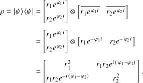
If you let ϕ = ϕ1 − ϕ2, this reduces to the previous case where we had already made the probability amplitude of |0⟩ real.
The density matrix of |ψ⟩ is independent of any global phase.
7.3.4 Observables and expectation
The matrices M0 = |0⟩⟨0| and M1 = |1⟩⟨1| are projectors and hence Hermitian matrices. If |ψ⟩ = a |0⟩ + b |1⟩,
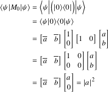
Similarly, ⟨ψ | M1 | ψ⟩ = |b|2.
To be explicit, ⟨ψ | M0 | ψ⟩ = |a|2 is the probability of measuring |0⟩ and ⟨ψ | M1 | ψ⟩ = |b|2 is the probability of measuring |1⟩.
The eigenvalues of M0 are 0 and 1, corresponding to eigenvectors |1⟩ and |0⟩, respectively. M1 has the same eigenvalues, with the eigenvectors reversed. M0 and M1 are both examples of observables: Hermitian matrices whose eigenvectors form a basis for the quantum state space.
Question 7.3.3
What is the relationship between the coefficients of the basis elements formed by the eigenvectors and the probabilities of seeing those basis elements when we measure?
Now let’s turn this around and suppose A is an observable. A is a Hermitian matrix with eigenvectors |e1⟩ and |e2⟩ corresponding to eigenvalues e1 and e2. |e1⟩ and e1 are different objects! We use |e1⟩ as the label for the eigenvector corresponding to e1. Also remember that an expression like ⟨e1 | ψ⟩ means ⟨e1||ψ⟩. It is not any sort of multiplication by e1.
By definition,
If |ψ⟩= a |e1⟩ + b |e2⟩ with ⟨ψ | ψ⟩ = 1, by the properties of the inner product,
Now that we have a set of values and corresponding probabilities for when we might get them, it is reasonable to talk about expectation as we first discussed in section 6.6 .
The expected value, or expectation, ⟨A⟩ of A given the state |ψ⟩ is
Question 7.3.4
Why does |⟨e1 | ψ⟩|2 = ⟨ψ | e1⟩ ⟨e1 | ψ⟩?
We can simplify this:

Question 7.3.5
What are ⟨M0⟩ and ⟨M1⟩ for |ψ⟩ = a |e1⟩ + b |e2⟩?
7.4 A non-linear projection
In chapter 5 we saw examples of linear projections, such as mapping any point in the real plane to the line y = x. Now we look at a special kind of projection that is non-linear. We map almost every point on the unit circle onto a line.
Here is a unit circle and the line y = −1 that sits right below it.
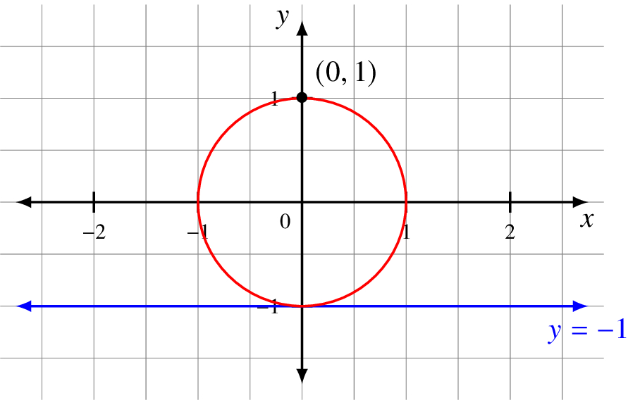
We can map every point on the circle except (0, 1), the north pole, to a point on the line y = −1. We simply draw a line from (0 ,1) through the point on the circle. The result is where that line intersects y = −1.

The point where it intersects the line is ![]() . We compute this using the slope-intercept form.
. We compute this using the slope-intercept form.
- We know two points on the line: the north pole (0, 1) and the point on the circle
 .
. - The slope m is the difference in y values divided by the difference in x values.

- When x = 0, y = 1. The equation of the line is
y = (√2 − 1)x + 1
- To see where it intersects the line y = −1, we just set y = −1 and solve.
−1 = (√2 − 1)x + 1and so−2 = (√2 − 1)xand so

By construction, the y coordinate is always −1.
Let’s generalize this to a point (x0, y0) on the circle.
- The slope is

- The line must intersect the y axis at (0, 1) and so the equation of the line is

- Setting y = −1 and solving for x yields
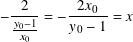
- The image of the projection is (−2 x0/(y0 − 1), −1).
Question 7.4.1
Does this generalized method give us the same answer we calculated earlier for ![]() ?
?
This general formula works for every point on the circle except for y0 = 1, the north pole.
Question 7.4.2
What point on the circle maps to (0, −1)?
Is this projection f invertible?
To construct f−1, we begin with an a in R. We want f−1(a) to be a point on the unit circle (x0, y0). What’s the most defining aspect of a point on the unit circle? It’s the relationship
- Given a, consider the point (a, −1) on the line y = −1.
- Draw the line from this point to the north pole (0, 1) and ask: where does this line intersect the unit circle?
- The slope m is −2/a (verify this and see the note below) and the full equation of the line is

- Squaring both sides:

- Substituting in x0 and y0:

- But x02 + y02 = 1!
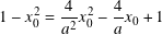
- Negating and moving the terms on the left side to the right and then simplifying:
- We can rule out x0 = 0 because this would give us the north pole. Therefore
or
 or
or

If a = 2 then x0 = 1. Trivially, y0 = 0. So f−1(2) = (1, 0).
What about if a = −4? Then x0 = −16/(4 + 16) = − 4/5. Given the equation of the unit circle from subsection 4.2.3,
By inspection of the graph,

When |a| ≥ 1 then y0 ≥ 0. Similarly, |a| < 1 implies y0 < 0. We conclusively conclude y0 = 3/5.
There were two problems with the above analysis. First, it’s not really acceptable to say ‘‘I looked at the graph and decided this was the situation.’’ Therefore, I leave it to you:
Question 7.4.3
Show algebraically that |a| ≥ 1 means y0 ≥ 0, and |a| < 1 means y0 < 0.
The second problem is much more serious. Though I said the ‘‘slope m of the line is −2/a,’’ I never said anything about a being non-zero.
The case a = 0 is special because it corresponds to the point directly under the north and south poles on y = −1. The line through the north pole is vertical and so is ∞. Here f−1(0) = (0, −1).
We can now fully describe f and f−1.
If f is the projection of a point (x0, y0), y0 ≠ 1, on the unit circle onto the line y = −1, then its image is (a, −1) where
The inverse function f−1(a) for an a in R is defined by

Our intermediate computations disallowed the case a = 0 though it is covered by the third case.
Though we did use trigonometry in the above analysis, we did not use angles. To conclude this section, let’s quickly recast what we worked out but this time give the point on the unit circle by its angle 0 ≤ θ < 2π rather than Cartesian coordinates.
We need to exclude θ = π/4 because this is the north pole. To keep our functions straight, we call this one g:
If g is the projection of a point given by an angle θ such that 0 ≤ θ < 2π, θ ≠ π/4, on the unit circle onto the line y = −1, then its image is (a, −1) where
What about g−1? In this example, we want to go from −4 to the value of θ.

Let θ = arccos(x0) = arccos(4a/(4 + a2)). By the definition of the inverse cosine, this has a value between 0 and π, inclusive. This alone does not tell us if the point is on the upper or lower half of the unit circle.
Let a be in R and θ = arccos(4a/(4 + a2)). The inverse function g−1(a) is defined by
In this projection, we took an object that lived in two dimensions but was determined by one variable θ and mapped it to the one-dimensional line R1. Here dimensions map to the idea of ‘‘degrees of freedom’’ as they would be expressed through the linear independence of a basis. Though the unit circle lives in R2, the relationship
7.5 The Bloch sphere
We describe the state of a qubit by a vector
The magnitudes r1 and r2 are related by r12 + r22 = 1. This is a mathematical condition. We saw in section 7.3 that it’s the relative phase of ϕ2 − ϕ1 that is significant and not the individual phases ϕ1 and ϕ2. This is a physical condition and it also means we can take a to be real.
We also saw that we could represent a quantum state as
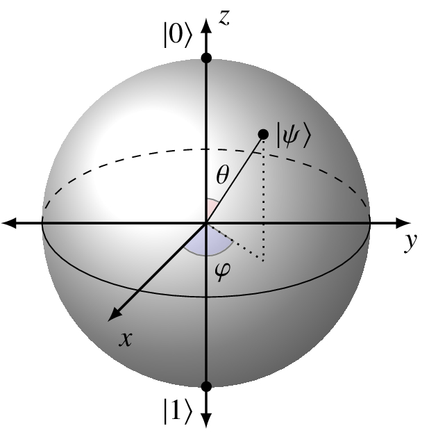
The two angles have the ranges 0 ≤ θ ≤ π and 0 ≤ ϕ < 2π. θ is measured from the positive z axis and ϕ from the positive x axis in the xy-plane.

The non-linear projection is from the three-dimensional surface of the hypersphere in C2, thought of as R4, to the two-dimensional surface of the Bloch sphere in R2. They key property that allows us to do this is that we can ignore global phase.
We start by asking ‘‘what are all the vectors in C2 of length 1?’’ to get the hypersphere. We then state ‘‘we’re going to say that any two points on the hypersphere are the ‘same’ if they are different only by a complex number multiple of magnitude 1.’’ With these properties and equivalences, along with some algebra and geometry, we get the points on the Bloch sphere as the possible quantum states of a qubit.
The eponymous sphere is named after Felix Bloch, a scientist who won the 1962 Nobel Prize in physics for his work in nuclear magnetic resonance (NMR). [2]
It’s easy to get confused here when we see |ψ⟩. Is this on the Bloch sphere or is it in C2? We do not distinguish these cases by notation and so I will make it clear by context.
Given a point/state on the Bloch sphere given by θ and ϕ, we can go back to |ψ⟩ = a |0⟩ + b |1⟩ in C2 by
On the other hand, if

Felix Bloch (1905-1983) in 1961. Photo subject to use via the Creative Commons Attribution 3.0 Unported license . [3]
If a = 0 then b = 1 and we have |1⟩. We map this to θ = π and ϕ = 0. If a = 1 then b = 0 and we have |0⟩, which goes to θ = 0 and ϕ = 0.
Assume neither a nor b is 0 and so the magnitudes r1 and r2 are positive real numbers. We rewrite
Since r12 + r22 = 1, the point (r1, r2) is on the unit circle in the first quadrant. We can identify an angle θ0 = arccos(r1) with 0 < θ0 < π/2 so that
Let’s go back to |0⟩ and |1⟩ and examine the choices we made above for θ and ϕ.
We cannot choose ϕ2 uniquely because of the multiplication by 0 in front of eϕ2 i. We might as well choose ϕ2 = ϕ1 and ϕ = 0.
Question 7.5.1
Are our choices θ = π and ϕ = 0 for |1⟩ also reasonable?
From all this, we have worked out the mappings to and from the Bloch sphere for qubit states in C2. |0⟩ maps to the north pole and |1⟩ maps to the south pole.
What about |+⟩ and |−⟩?
Question 7.5.2
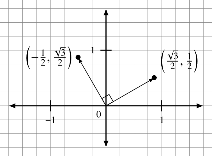
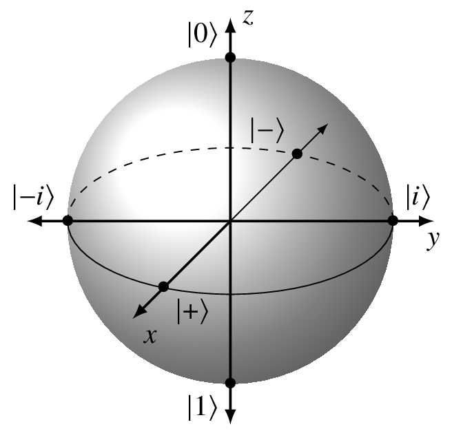
Show |+⟩ maps to θ = π/2 and ϕ = 0 on the Bloch sphere. Then show |−⟩ maps to θ = π/2 and ϕ = π. What are these points using Cartesian coordinates in R3?
The kets |0⟩ and |1⟩ lie on the z axis and |+⟩ and |−⟩ lie on the x axis.
What is the orthonormal basis that would lie on the y axis? Let’s call them |A⟩ and |B⟩ for now.
The two points in which we are interested have Cartesian coordinates (0, 1, 0) and (0, −1, 0).

For each of them we can take θ = π/2. For |A⟩, we use ϕ = π/2, and for |B⟩, ϕ = 3π/2 gets us to (0, −1, 0).
Now we use these to go back to |ψ⟩ = a |0⟩ + b |1⟩ in C2. We set

So
Question 7.5.3
Verify |i⟩ and |−i⟩ are orthonormal.
From the evidence we’ve seen in three cases so far, an orthonormal basis in C2 maps to two opposite points on the Bloch sphere. Start thinking about why this is the case.
Every quantum state on the equator has an equal probability of producing |0⟩ or |1⟩ when measured. That is, if a state is on the equator then in terms of its coordinates a and b in a |0⟩ + b |1⟩ in C2, |a|2 = |b|2 = 0.5.
Naturally, the state |0⟩ has probability 1.0 of yielding itself when measured and probability 0.0 of producing |1⟩. These probabilities are reversed for |1⟩.
For a latitude on the Bloch sphere that is not the equator, the probabilities of collapsing to |0⟩ or |1⟩ are different but still add up to 1.0. The probability of yielding |0⟩ is the same for every point on that latitude. Ditto for |1⟩.

We have now seen three pairs of basis elements and they go by different names:
| Basis | Common name | Bloch sphere axis name |
| {|0⟩, |1⟩} | Computational | Z |
| {|+⟩, |−⟩} | Hadamard | X |
| {|i⟩, |−i⟩} | Circular | Y |
The Y basis is the same as the circular basis. In this case we also have the alternative notation |i⟩ = |↻⟩ and |−i⟩ = |↺⟩.
7.6 Professor Hadamard, meet Professor Pauli
Other than mapping the state of a qubit to a Bloch sphere and so looking at it in a different way, what can you do with a qubit? In this section we look at the operations, also called gates, you can apply to a single qubit. Later we expand our exploration to gates that have multiple qubits as inputs and outputs. In chapter 9 we build circuits with these gates to implement algorithms.
Here, for example, is a circuit with one qubit initialized to |0⟩ that performs one operation, X, and then measures the qubit.

Gates are always reversible, but some other operations are not. This comes from quantum mechanics and gates corresponding to unitary transformations. Measurement is irreversible, and so is the |0⟩ reset operation described in subsection 7.6.13.
When I include the measurement operation in a circuit in the next chapter and beyond, it looks like the graphic below.

Measurement returns a |0⟩ or |1⟩. Mathematically, we do not worry about how it happens other than the probability. In chapter 11 I discuss how measurement is done in the different physical qubit technologies.
Since a qubit state is a two-dimensional complex ket, or vector, all quantum gates have 2 by 2 matrices with complex entries according to some basis. This makes them small and very easy to manipulate. They are unitary matrices.
If A is a complex square matrix then it is unitary if its adjoint A† is also its inverse A−1. Hence A A† = A† A = I.
This means the columns of A are orthonormal, as are the rows.
|det(A)| = 1.
Note the last statement says the absolute value of the determinant is 1, not that the determinant is 1. Since it is in C, the determinant is of the form eϕ i for 0 ≤ ϕ < 2π.
The remainder of this section is a catalog of some of the most useful and commonly used 1-qubit quantum gates. As you will see, there is often more than one way to accomplish the same qubit state change. Why you would want to do so is the topic of chapter 9.
When we looked at classical circuits in section 2.4 , only the not operation was reversible. That’s also the only operation which carries over to quantum. We start there.
7.6.1 The quantum X gate
The X gate has the matrix
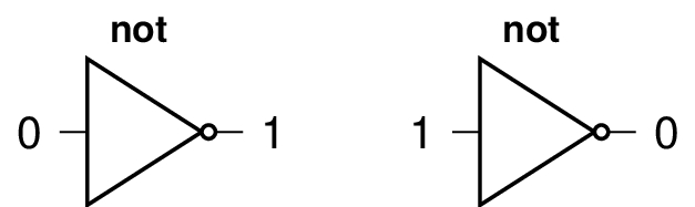
The not gate is a ‘‘bit flip’’ and by analogy we also say X is a bit flip.
For |ψ⟩ = a |0⟩ + b |1⟩ in C2,
In terms of the Bloch sphere, the X gate rotates by π around the x axis. So not only are the poles flipped but points in the lower hemisphere move to the upper and vice versa.
Since X X = I2, the X gate is its own inverse. This is reasonable because in the classical case it is also true that not ○ not is the identity operation.
When we considered rotations we saw that the matrix for R3 that does a rotation around the x axis by θ radians works like


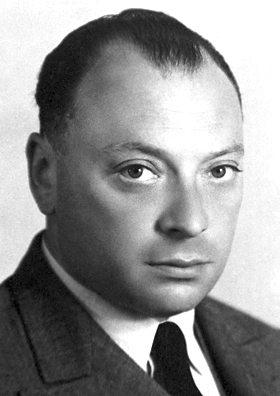
The physicist Wolfgang Pauli, 1900-1958. Pauli won the Nobel Prize in Physics in 1945. Photo is in the public domain.


Question 7.6.1
What does the X gate do to |i⟩ and |−i⟩?
Question 7.6.2
What are the eigenvectors and eigenvalues of σx?

The input state enters on the left, the X unitary transformation is applied, and the new quantum state result comes out the right side.
7.6.2 The quantum Z gate
The Z gate has the matrix
Question 7.6.3
Show by calculation that X Z = − Z X.
Since Z Z = I2, the Z gate is its own inverse. If you rotate by π and then rotate by π again, you end up back where you started.
For |ψ⟩ = a |0⟩ + b |1⟩ in C2,
In C2, σz has eigenvalues +1 and −1 for eigenvectors |0⟩ and |1⟩, respectively. Per subsection 7.3.4, Z or σz is the observable for the standard computational basis |0⟩ and |1⟩.
Remember that |1⟩ and −|1⟩ = eπ i |1⟩ in C2 map to the same point we are also calling |1⟩ on the Bloch sphere. If we express
| σz |ψ⟩ | = r1 eθ1 i |0⟩ − r2 eθ2 i |1⟩ |
| = r1 eθ1 i |0⟩ + eπ i r2 eθ2 i |1⟩ | |
| = r1 eθ1 i |0⟩ + r2 e(π + θ2) i |1⟩ | |
| = eθ1 i (r1 |0⟩ + r2 e(π + θ2 − θ1) i |1⟩) |
The relative phase of |ψ⟩ is changed to π plus that relative phase, adjusted to be between 0 and 2π. This is a phase flip and Z is called a phase flip gate. Since it reverses the sign of the second amplitude, it is also called a sign flip gate.
When I include the Z gate in a circuit it looks like the graphic below.

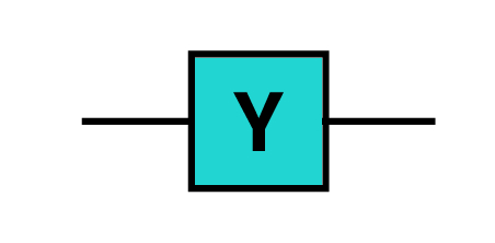
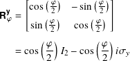
7.6.3 The quantum Y gate
The Y gate has the matrix
Question 7.6.4
Show by calculation that X Y = −Y X and Z Y = −Y Z.
Since Y Y = I2, the Y gate is its own inverse.
For |ψ⟩ = a |0⟩ + b |1⟩ in C2,
If |ψ⟩ = a |0⟩ + b |1⟩ in C2, then a bit flip interchanges the coefficients of |0⟩ and |1⟩. A phase flip changes the sign of the coefficient of |1⟩. A simultaneous bit and phase flip does both:
Question 7.6.5
What is the 3 by 3 rotation matrix for the Y gate?
7.6.4 The quantum ID gate
The ID gate does nothing and is typically used when constructing or drawing circuits where we want to show something happening to every qubit at every step. If we did construct an implementation, it would be multiplication by I2, the 2 by 2 identity matrix.
When I include the ID gate in a circuit it looks like the graphic below.

The ID gate is also used in circuits to indicate a place to pause or delay. This allows, for example, researchers to calculate ?? of a qubit.
7.6.5 The quantum H gate
The H gate, or H⊗1 or Hadamard gate, has the matrix
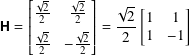
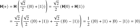
The Hadamard gate is one of the most frequently used gates in quantum computing. H is often the first gate applied in a circuit. When you read ‘‘put the qubit in superposition’’ it usually means ‘‘take the qubit initialized in the |0⟩ state and apply H to it.’’
The Hadamard matrix is the change of basis matrix from {|0⟩, |1⟩} to {|+⟩, |−⟩}.
Since HH = I2, the H gate is its own inverse.
Question 7.6.6
What is the 3 by 3 matrix for the H gate on the Bloch sphere? It is the product of two 3 by 3 rotation matrices. What are they?

The mathematician Jacques Hadamard, 1865-1963. Photo is in the public domain.
When I include the H gate in a circuit it looks like the graphic below.

In quantum computing there are a lot of zeroes and ones floating around. We use these in interesting ways. For example, suppose we have |x⟩ where x is either 0 or 1. Thinking of x as being in Z, look at expressions like (−1)x, which is 1 or −1 as x is 0 or 1.
For our H gate, we can stare at
Question 7.6.7
Show using matrix calculations that X = H Z H.
A change of basis from the computational basis {|0⟩, |1⟩} to the Hadamard basis {|+⟩, |−⟩} changes a bit flip X to a phase flip Z.
Question 7.6.8
What is H X H?
7.6.6 The quantum Rϕz gates
We can generalize the phase changing behavior of the Z gate by noting
Question 7.6.9
What is the 3 by 3 rotation matrix for ![]() ? For Z?
? For Z?
The inverse of ![]() is
is ![]() .
.
![]() = ID.
= ID.
![]() = Z.
= Z.
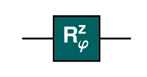
An alternative form of the matrix for ![]() is
is
7.6.7 The quantum S gate
The S gate is a shorthand for ![]() . After applying, the phase is adjusted to be greater than or equal to 0 and less than 2π.
. After applying, the phase is adjusted to be greater than or equal to 0 and less than 2π.
Question 7.6.10
What is the 3 by 3 rotation matrix for the S gate?
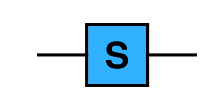
Traditionally and confusingly, the S gate is also known as the π/4 gate. This is because we can express the matrix in this way:
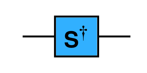
7.6.8 The quantum S† gate
The S† gate is a shorthand for ![]() =
= ![]() . After applying, the phase is adjusted to be greater than or equal to 0 and less than 2π.
. After applying, the phase is adjusted to be greater than or equal to 0 and less than 2π.
Question 7.6.11
What is the 3 by 3 rotation matrix for the S† gate?
7.6.9 The quantum T gate
The T gate is a shorthand for ![]() . After applying, the phase is adjusted to be greater than or equal to 0 and less than 2π.
. After applying, the phase is adjusted to be greater than or equal to 0 and less than 2π.
Question 7.6.12
What is the 3 by 3 rotation matrix for the T gate?
When I include the T gate in a circuit it looks like the graphic below.

The T gate is also known as the π/8 gate. We can write its matrix as
7.6.10 The quantum T† gate
The T† gate is a shorthand for ![]() =
= ![]() . After applying, the phase is adjusted to be greater than or equal to 0 and less than 2π.
. After applying, the phase is adjusted to be greater than or equal to 0 and less than 2π.

Question 7.6.13
What is the 3 by 3 rotation matrix for the T† gate?
When I include the T† gate in a circuit it looks like the graphic below.

7.6.11 The quantum Rϕx and Rϕy gates
Just as ![]() is an arbitrary rotation around the z axis, we can define gates that rotate around the x and y axes.
is an arbitrary rotation around the z axis, we can define gates that rotate around the x and y axes.

and

where I2 is the 2 by 2 identity matrix, σx is the Pauli X matrix, and σy is the Pauli Y matrix.
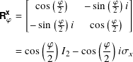
7.6.12 The quantum √NOT gate
Another gate used in some of the quantum computing literature is the ‘‘square root of NOT’’ gate. It has the matrix

The X gate is the quantum version of not, and that’s how this gate gets its name.
Question 7.6.14
Show that ![]() is unitary. What is its determinant? What does it do to |0⟩ and |1⟩?
is unitary. What is its determinant? What does it do to |0⟩ and |1⟩?
The adjoint of this gate has matrix
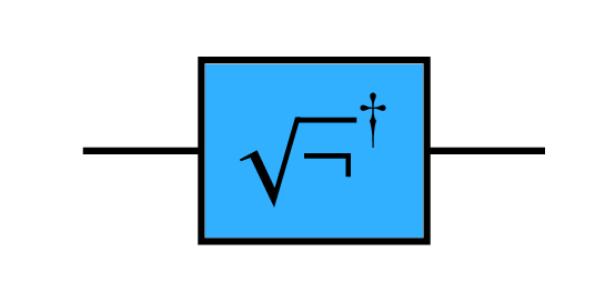
7.6.13 The quantum |0> RESET operation
Though it is not a reversible unitary operation, and hence not a gate, some quantum computing software environments allow you to reset a qubit in the middle of a circuit to |0⟩, Use of this operation may make your code non-portable.

7.7 Gates and unitary matrices
The collection of all 2 by 2 unitary matrices (subsection 5.7.5 ) with entries in C form a group under multiplication called the unitary group of degree 2. It is denoted by U(2, C). It is a subgroup of GL(2, C), the general linear group of degree 2 over C.
Every 1-qubit gate corresponds to such a unitary matrix. We can create all 2 by 2 unitary matrices from the identity and Pauli matrices.
Any U in U(2, C) can be written as a product of a complex unit times a linear combination of unitary matrices
- I2 is the 2 by 2 identity matrix
- cσx cσy, and cσz are Pauli matrices
- 0 ≤ θ < 2π
- cI2 is in R
- cσx, cσy, and cσz are in C
- |cI2|2 + |cσx|2 + |cσy|2 + |cσz|2 = 1
- Re(cI2) cσx + Im(cσy) cσz = 0
- Re(cI2) cσy + Im(cσx) cσz = 0
- Re(cI2) cσz + Im(cσx) cσy = 0
The complex unit only affects the global phase of the qubit state and so is not observable. This means that we do not see its effect when we measure because it does not affect the probabilities of seeing one thing or another. [4]
Question 7.7.1
What does this mean in terms of the ID, X, Y, and Z gates?
7.8 Summary
The quantum states of a qubit are the unit vectors in C2, where we identify two states as being equivalent if they differ only by a multiple of a complex unit. To better visualize actions on a qubit, we introduced the Bloch sphere in R3 and showed where special orthonormal bases map onto the sphere.
Any new idea seems to deserve its own notation and we did not disappoint when we introduced Dirac’s bra-ket representation of vectors. This significantly simplifies calculation when working with multiple qubits.
Given the ket form of qubit states, we introduced the standard 1-qubit gate operations. In the classical case in section 2.4 , there was only one operation we could perform on a single bit, not. In the quantum case, there are many, in fact an infinite number, of single qubit operations.
We next look at how to work with two or more qubits and the quantum gates that operate on them. We also introduce entanglement, an essential notion from quantum mechanics.
References
- [1]
-
Karen Barad. Meeting the Universe Halfway. Quantum Physics and the Entanglement of Matter and Meaning. 2nd ed. Duke University Press Books, 2007.
- [2]
-
F. Bloch. ‘‘Nuclear Induction’’. In: Physical Review 70 (7-8 Oct. 1946), pp. 460–474.
- [3]
-
Creative Commons. Attribution 3.0 Unported (CC BY 3.0) . url: https://creativecommons.org/licenses/by/3.0/legalcode.
- [4]
-
Simon J. Devitt, William J. Munro, and Kae Nemoto. ‘‘Quantum error correction for beginners’’. In: Reports on Progress in Physics 76.7, 076001 (July 2013), p. 076001.
- [5]
-
P. A. M. Dirac. The Principles of Quantum Mechanics. Clarendon Press, 1930.
- [6]
-
A. Yu. Kitaev, A. H. Shen, and M. N. Vyalyi. Classical and Quantum Computation. American Mathematical Society, 2002.