6
What Do You Mean ‘‘Probably’’?
Any one who considers arithmetical methods of producing
random digits is, of course, in a state of sin.
Here’s the key to what we’re going to cover in this chapter: in any given situation, the sum of the probabilities of all the different possible things that could happen always add up to 1.
In this short chapter, I cover the basics of practical probability theory to get us started on quantum computing and its applications.
Topics covered in this chapter
6.2 More formally
6.3 Wrong again?
6.4 Probability and error detection
6.5 Randomness
6.6 Expectation
6.7 Markov and Chebyshev go to the casino
6.8 Summary
6.1 Being discrete
Sometimes it seems like probability is the study of flipping coins or rolling dice, given the number of books that explain it those ways. It’s very hard to break away from these convenient examples. An advantage shared by both of them is that they make it is easy to explain discrete events and independence.
For the sake of mixing it up, suppose we have a cookie machine. It’s a big box with a button on top. Every time you press the button, a cookie pops out of a slot on the bottom. There are four kinds of cookies: chocolate, sugar, oatmeal, and coconut.
Assume for the moment there is no limit to the number of cookies our machine can distribute. If you hit the button a million times, you get a million cookies. Also assume you get a random cookie each time. What does this mean, ‘‘random’’?
Without a rigorous definition, random here means that the odds of getting any one of the cookies is the same as getting any other. That is, roughly one-fourth of the time I would get chocolate, one-fourth of the time I would get sugar, one-fourth for oatmeal, and one-fourth coconut.
The probability of getting a sugar cookie, say, is 0.25 and the sums of the probabilities for all the cookies is 1.0. Since there are four individual and separate possible outcomes, we say this is a discrete situation. We write this as
Question 6.1.1
What is the probability of my not getting a coconut cookie on one push of the button?
Now let’s change this situation. Last time the cookie service-person came, they accidentally loaded the coconut slot inside the machine with chocolate cookies. This changes the odds:
| P(chocolate) = 0.5 | P(sugar) = 0.25 | |
| P(oatmeal) = 0.25 | P(coconut) = 0 . |
The sum of the probabilities is still 1, as it must be, but the chance of getting a chocolate cookie is now twice as large as it was. The probability of getting a coconut cookie is 0, which is another way of saying it is impossible.
Had the service person simply forgotten to fill the coconut slot, we would have
| P(chocolate) = 0.3 | P(sugar) = 0.3 | |
| P(oatmeal) = 0.3 | P(coconut) = 0 . |
Since we are only talking about probabilities, it is quite possible for me to get three chocolate cookies in a row after I hit the button three times. We do not have enough data points for the observed results to be consistently close to the probabilities. It is only when I perform an action, in this case pressing the button many, many times, that I will start seeing the ratio of the number of times I saw the desired event to the total number of events approach the probability.
If I press the button 100 times I might see the following numbers
| Kind of cookie | Number of times seen | Ratio of seen/100 |
| chocolate | 22 | 0.22 |
| sugar | 26 | 0.26 |
| oatmeal | 25 | 0.25 |
| coconut | 27 | 0.27 |
Assuming everything is as balanced as I think, I’ll eventually be approaching the probabilities. If I instead saw
| Kind of cookie | Number of times seen | Ratio of seen/100 |
| chocolate | 0 | 0.0 |
| sugar | 48 | 0.48 |
| oatmeal | 52 | 0.52 |
| coconut | 0 | 0.0 |
I would rightfully suspect something was wrong. I would wonder if there were roughly the same number of sugar and oatmeal cookies in the machine but no chocolate or coconut cookies. When experimentation varies significantly from prediction, it makes sense to examine your assumptions, your hardware, and your software.
Now let’s understand the probabilities of getting one kind of cookie followed by another. What is the probability of getting an oatmeal cookie and then a sugar cookie?
This is
| P(oatmeal and then sugar) | = P(oatmeal) × P(sugar) |
| = 0.25 × 0.25 = 0.0625 = 1/16. |
| chocolate + chocolate | chocolate + sugar | chocolate + oatmeal | chocolate + coconut |
| sugar + chocolate | sugar + sugar | sugar + oatmeal | sugar + coconut |
| oatmeal + chocolate | oatmeal + sugar | oatmeal + oatmeal | oatmeal + oatmeal |
| coconut + chocolate | coconut + sugar | coconut + oatmeal | coconut + coconut |
Getting oatmeal and then sugar is one of the sixteen choices.
What about ending up with one oatmeal and one sugar cookie? Here it doesn’t matter which order the machine gives them to me. Two of the sixteen possibilities yield this combination and so
Question 6.1.2
What is the probability of my getting a chocolate cookie on the first push of the button and then my not getting a chocolate cookie on the second?
6.2 More formally
In the last section, there were initially four different possible outcomes, those being the four kinds of cookies that could pop out of our machine. In this situation, our sample space is the collection
The sample space for getting one cookie and then another has size 16. A probability distribution assigns a probability to each of the possible outcomes, which are the values of the random variable. The probability distribution for the basic balanced case is
| chocolate → 0.25 | sugar → 0.25 | |
| oatmeal → 0.25 | coconut → 0.25 . |
When the probabilities are all equal, as in this case, we have a uniform distribution.
If our sample space is finite or at most countably infinite, we say it is discrete. A set is countably infinite if it can be put in one-to-one correspondence with Z. One way to think about it is that you are looking at an infinite number of separate things with nothing between them.
The sample space is continuous if it can be put in correspondence with some portion of R or a higher dimensional space. As you boil water, the sample space of its temperatures varies continuously from its starting point to the boiling point. Just because your thermometer only reads out decimals, it does not mean the temperature itself does not change smoothly within its range.
This raises an important distinction. Though the sample space of temperatures is continuous, the sample space of temperatures as read out on a digital thermometer is discrete, technically speaking. It is represented by the numbers the thermometer states, to one or two decimal places. The discrete sample space is an approximation to the continuous one.
When we use numeric methods on computers for working in such situations, we are more likely to use continuous techniques. These involve calculus, which I have not made a prerequisite for this book, and so will not cover. We do not need them for our quantum computing discussion.
Our discrete sample spaces will usually be the basis vectors in complex vector spaces of dimension 2n.
6.3 Wrong again?
Suppose you have a very faulty calculator that does not always compute the correct result.
If the probability of getting the wrong answer is p, the probability of getting the correct answer is 1 − p. This called the complementary probability. Assuming there is no connection between the attempts, the probability of getting the wrong answer two times in a row is p2 and the probability of getting the correct answer two times in a row is (1 − p)2.
Question 6.3.1
Compute p2 and (1 − p)2 for p = 0, p = 0.5, and p = 1.0.
To make this useful, we want the probability of failure p to be non-zero.
For n independent attempts, the probability of getting the wrong answer is pn. Let’s suppose p = 0.6. We get the wrong answer 60% of the time in many attempts. We get the correct answer 40% of the time.
After 10 attempts, the probability of having gotten the wrong answer every time is 0.610 ≈ 0.006.
On the other hand, suppose I want to have a very low probability of having always gotten the wrong answer. It’s traditional to use the Greek letter ε (pronounced ‘‘epsilon’’) for small numbers such as error rates. For example, I might want the chance of never having gotten the correct answer to be less than ε = 10−6 = 0.000001.
For this, we solve
6.4 Probability and error detection
Let’s return to our repetition code for error detection from section 2.1 . The specific example I want to look at is sending information that is represented in bits. The probability that I will get an error by flipping a 0 to a 1 or a 1 to a 0 is p. The probability that no error occurs is 1 - p, as above.
This is called a binary symmetric channel. We have two representations for information, the bits, and hence ‘‘binary.’’ The probability of something bad happening to a 0 or 1 is the same, and that’s the symmetry.
Here is the scheme:
- Create a message to be sent to someone.
- Transform that message by encoding it so that it contains extra information. This will allow it to be repaired if it is damaged en route to the other person.
- Send the message. ‘‘Noise’’ in the transmission may introduced errors in the encoded message.
- Decode the message, using the extra information stored in it to try to fix any transmission errors.
- Give the message to the intended recipient.

For this simple example, I send a single bit and I encode it by making three copies. This means I encode 0 as 000 and 1 as 111.
The number of 1s in an encoded message (with or without errors) is called its weight. The decoding scheme is
| 000 | 001 | 010 | 100 | 111 | 101 | 110 | 101 |
If there are more 0s than 1s, I decode, or ‘‘fix,’’ the message by making the result 0. Similarly, if there are more 1s than 0s, I decode the message by making the result 1. The result of decoding will be the original if at most one error occurred, in this case. This is why we made an odd number of copies.
The first four would all be correctly decoded as 0 if that’s what I sent. They either have zero or only one errors. The last four are the cases where two or three errors occurred.
Question 6.4.1
What’s the similar observation if I had sent 1?
Now assume I sent 0. There is one possible received message, 000, where no error popped up and that has probability (1 − p)3.
There are three results with one error and two non-errors: 001, 010, and 100. The total probability of seeing one of these is
In total, the probability that I receive the correct message or can fix it to be correct is
If p = 1.0, this probability is 0, as you would expect. We can’t fix anything. If p = 0.0, there are no errors and the probability of ending up with the correct message is 1.0.
If there is an equal chance of error or no error, p = 0.5 and then so too is the probability we can repair the message 0.5. If the chance of error in one in ten, p = 0.1, the probability that it was correct or we can fix is 0.972.

Question 6.4.2
What is the maximum value of p I can have so that my chance of getting the right message or being able to correct it is 0.9999?
6.5 Randomness
Many programming languages have functions that return pseudo-random numbers. The prefix ‘‘pseudo’’ is there because they are not truly random numbers but nevertheless do well on statistical measurements of how well-distributed the results are.
Given four possible events E0, E1, E2, and E3 with associated probabilities p0, p1, p2, and p3, how might we use random numbers to simulate these events happening?
Suppose
random() function returns a random real number r such that 0.0 ≤ r < 1.0. Based on the value of r we get, we determine that one of the E0, E1, E2, and E3 events occurred.
If you are not using Python, use whatever similar function is available in your programming language and environment.
The general scheme is to run the following steps in order:
- r < p0 then we have observed E0 and we stop. In the example, p0 = 0.15. If not, ...
- If r < p0 + p1 then we have observed E1 and we stop. If not, ...
- If r < p0 + p1 + p2 then we have observed E2 and we stop. If not, ...
- If r < p0 + p1 + p2 + p3 then we have observed E3 and we stop.
#!/usr/bin/env python3
import random
example_probabilities = [0.15, 0.37, 0.26, 0.22]
def sample_n_times(probabilities, n):
probability_sums = []
number_of_probabilities = len(probabilities)
sum = 0.0
for probability in probabilities:
sum += probability
probability_sums.append(sum)
counts = [0 for probabilities in probabilities]
for _ in range(n):
r = random.random()
for s,j in zip(probability_sums, range(number_of_probabilities)):
if r < s:
counts[j] = counts[j] + 1
break
print(f"nResults for {n} simulated samples")
print("nEvent Actual Probability Simulated Probability")
for j in range(number_of_probabilities):
print(f" {j}{14*’ ’}{probabilities[j]}{20*’ ’}"
f"{round(float(counts[j])/n, 4)}")
sample_n_times(example_probabilities, 100)
sample_n_times(example_probabilities, 1000000)
The code in Listing 6.1 simulates this sampling a given number of times. On one run for 100 samples, I saw the events distributed in this way:
Results for 100 simulated samples

Event     Actual Probability     Simulated Probability
  0              0.15                    0.11
  1              0.37                    0.36
  2              0.26                    0.29
  3              0.22                    0.24
The values are close but not very close. It’s probability, after all.
Significantly increasing the number of samples to 1 million produced values much closer to the expected probabilities.
Results for 1000000 simulated samples

Event     Actual Probability     Simulated Probability
  0              0.15                    0.1507
  1              0.37                    0.3699
  2              0.26                    0.2592
  3              0.22                    0.2202
If you plan to run this frequently, you should ensure you are not always getting the same sequence of random numbers. However, sometimes you do want a repeatable sequence of random numbers so that you can debug your code. In this situation, you want to begin with a specific random ‘‘seed’’ to initialize the production of numbers. In Python this function is seed().
Interestingly enough, one potential use of quantum technology is to generate truly random numbers. It would be odd to use a quantum device to simulate quantum computing in an otherwise classical algorithm!
To learn more
When I talk about Python in this book I always mean version 3. The tutorial and reference material on the official website is excellent. [6] There are many good books that teach how to code in this important, modern programming language for systems, science, and data analysis. [4] [5]
6.6 Expectation
Let’s look at the numeric finite discrete distribution of the random variable X with probabilities given in the table below.
If the process that is producing these values continues over time, what value would we ‘‘expect’’ to see?
| Value | Probability |
| 2 | 0.14 |
| 5 | 0.22 |
| 9 | 0.37 |
| 13 | 0.06 |
| 14 | 0.21 |
If they all have the same probability of occurring, the expected value, or expectation, ![]() is their average:
is their average:
If X is a random variable with values {x1, x2, ..., xn} and corresponding probabilities pk such that p1 + p2 + ··· + pn = 1, then
How much do the values in X differ from the expected value E(X)? For a uniform distribution, the average of the amounts each xk varies from E(X) is

The notation (X − E(X))2 refers to the new set of values (xk − E(X))2 for each xk in X.
The notation σ2(X) is often used instead of Var(X). The standard deviation σ of X is the square root of the variance √Var(X)
For a coin flip, ![]() with p1 = p2 = 0.5. Then
with p1 = p2 = 0.5. Then
Basically, I’m doing the same thing many times, with the same probabilities, and there are no connections between the Xj. The answer I get for any one Xj is independent of what happens for any other.
We return to expectation in the context of measuring qubits in subsection 7.3.4 .
6.7 Markov and Chebyshev go to the casino
In this section we work through the math from estimating π in section 1.5 . We dropped coins into a square and looked at how many of them had their centers on or inside a circle.
There are two important inequalities involving expected values, variances, and error terms. Let X be a finite random variable with distribution so that
Markov’s Inequality: For a real number a > 0,
In Markov’s Inequality, the expression P(X > a) means ‘‘look at all the xk in X and for all those where xk > a, add up the pk to get P(X > a).’’
Question 6.7.1
Show that Markov’s Inequality holds for the distribution at the beginning of this section for the values a = 3 and a = 10.
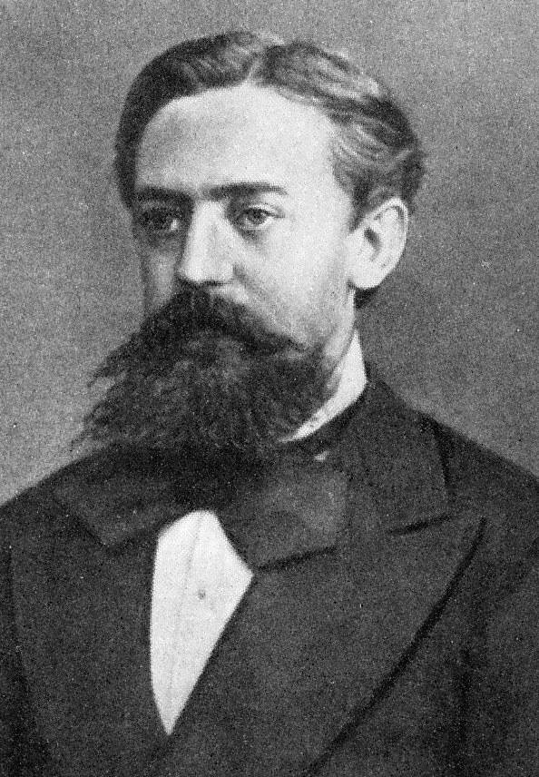
Andrey Markov, circa 1875. Photo is in the public domain.
Chebyshev’s Inequality: For any finite random variable X with distribution, and real number ε > 0,
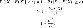
In Chebyshev’s Inequality, the expression P(|X − E(X)|) ≥ ε means ‘‘look at all the xk in X and for those whose distance from the expected value ![]() is greater than or equal to ε, add up the pk to get P(|X − E(X)|) ≥ ε.’’ Think of ε as an error term related to the probability of being away from the expected value.
is greater than or equal to ε, add up the pk to get P(|X − E(X)|) ≥ ε.’’ Think of ε as an error term related to the probability of being away from the expected value.
From Chebyshev’s Inequality we get a result which is useful when we are taking samples Xj, such as coin flips or the Monte Carlo samples described in section 1.5 .
Weak Law of Large Numbers: Let the set of Xj for 1 ≤ j ≤ n be independent identical random variables with identical distributions. Let μ = E(Xj), which is the same for all j. Then
What does this tell us about the probability of getting 7 or fewer heads when I do ten coin flips? Remember that in this case μ = 1/2 and σ2 = 1/4.


Pafnuty Chebyshev, circa 1890. Image is in the public domain.
Here we use ε = 1/5. The probability of getting 7 or fewer heads in 10 flips is greater than or equal to 0.15625.
Question 6.7.2
Repeat the calculation for 70 or fewer heads in 100 flips, and 700 or fewer heads in 1000 flips.
In section 1.5 we started using a Monte Carlo method to estimate the value of π by randomly placing coins in a 2 by 2 square in which is inscribed a unit circle. It’s easier to use the language of points instead of coins, where the point is the center of the coin.
The plot below uses 200 random points and yields 3.14 as the approximation.

Let’s now analyze this in the same way we did for the coin flips. In this case,
So X1 is dropping the first random point into the square and X1000000 is dropping the one millionth. The value is 1 for either of these if the point is in the circle. We have
The expected value ![]() is therefore this probability. For the variance,
is therefore this probability. For the variance,
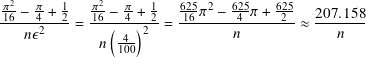
If we repeat the calculation and want the probability of the estimate being off by at most 0.0001 = 1/10000, we need n ≥ 2071576. Said another way, we need n this large to get the estimate this close with probability 99.9999%,
Finally, if want the probability of the estimate to π being off by at most 0.00001 = 10−5 (in the fifth decimal place) to be less than 0.0001 = 1/10000, we need n ≥ 82863028.
As you can see, we need many points to estimate π accurately to a small number of digits, in the last case more than 82 million points.
6.8 Summary
In this chapter we covered the elements of probability necessary for our treatment of quantum computing and its applications. When we work with qubits and circuits in the next two chapters we use discrete sample spaces, though they can get quite large. In these cases, the sizes of the sample spaces will be powers of 2.
Our goal in quantum algorithms is to adjust the probability distribution so that the element in the sample space with the highest probability is the best solution to some problem. Indeed, the manipulation of probability amplitudes leads us to find what we hope is the best answer. My treatment of algorithms in chapter 9 and chapter 10 does not go deeply into probability calculations, but does so sufficiently to give you an idea of how probability interacts with interference, complexity, and the number of times we need to run a calculation to be confident we have seen the correct answer.
To learn more
There are hundreds of books about probability and combination texts covering probability and statistics. These are for the applied beginner all the way to the theoretician, with several strong and complete treatments. [1]
Probability has applications in many areas of science and engineering, including AI/machine learning and cryptography. [3] [2, Chapter 5]
An in-depth understanding of continuous methods requires some background in differential and integral calculus.
References
- [1]
-
D.P. Bertsekas and J.N. Tsitsiklis. Introduction to Probability. 2nd ed. Athena Scientific optimization and computation series. Athena Scientific, 2008.
- [2]
-
Thomas H. Cormen et al. Introduction to Algorithms. 3rd ed. The MIT Press, 2009.
- [3]
-
Jeffrey Hoffstein, Jill Pipher, and Joseph H. Silverman. An Introduction to Mathematical Cryptography. 2nd ed. Undergraduate Texts in Mathematics 152. Springer Publishing Company, Incorporated, 2014.
- [4]
-
Mark Lutz. Learning Python. 5th ed. O’Reilly Media, 2013.
- [5]
-
Fabrizio Romano. Learn Python Programming. 2nd ed. Packt Publishing, 2018.
- [6]
-
The Python Software Foundation. Python.org. url: https://www.python.org/.
- [7]
-
John von Neumann. ‘‘Various techniques used in connection with random digits’’. In: Monte Carlo Method. Ed. by A.S. Householder, G.E. Forsythe, and H.H. Germond. National Bureau of Standards Applied Mathematics Series, 12, 1951, pp. 36–38.