11
Getting Physical
The non-physicist finds it hard to believe that really
the ordinary laws of physics, which he regards as the
prototype of inviolable precision,
should be based on the statistical tendency of matter
to go over into disorder.
It’s now time to discuss some considerations about how we go from theoretical mathematics and physics to the applied and experimental.
The qubits we make in the lab for research and those we will create for commercial use are physical hardware devices. As such, they are subject to noise from the environment, electronic components, and manufacturing choices. Hardware improvements decrease the disturbances, but software and system ones can too. The long-term goal is to have fully error corrected, fault-tolerant quantum computing devices.
Since we’re talking about physics, I explain the questionable fate of Schrödinger’s cat.
Topics covered in this chapter
11.2 What does it take to be a qubit?
11.3 Light and photons
11.3.1 Photons
11.3.2 The double-slit experiment
11.3.3 Polarization
11.4 Decoherence
11.4.1 T1
11.4.2 T2 and T2*
11.4.3 Pure versus mixed states
11.5 Error correction
11.5.1 Correcting bit flips
11.5.2 Correcting sign flips
11.5.3 The 9-qubit Shor code
11.5.4 Considerations for general fault tolerance
11.6 Quantum Volume
11.7 The software stack and access
11.8 Simulation
11.8.1 Qubits
11.8.2 Gates
11.8.3 Measurement
11.8.4 Circuits
11.8.5 Coding a simulator
11.9 The cat
11.10 Summary
11.1 That’s not logical
The qubits like those in the last two chapters are examples of ‘‘logical qubits.’’ We can use them indefinitely, they never lose state when they are not used, and we can apply as many gates to them as we wish.
When you build a quantum computer, the fundamental physical implementations of qubits aren’t as perfect as logical qubits. Such a qubit, called a ‘‘physical qubit,’’ starts to lose its ability to hold onto a state after what is called its ‘‘coherence time.’’ We also say that the qubit is decohering.
It’s a goal of quantum computing researchers and engineers to delay the decay of a physical qubit’s quantum state as long as possible. Since the decay is inevitable, a goal of fault tolerance and error correction is to handle and fix the effects of the qubits’ decoherence throughout the execution of a circuit.
Is it possible to create objects that act like logical qubits from physical ones? Research today says ‘‘yes’’ but it will require hundreds to thousands of physical qubits to make one logical qubit. When we get there, we will have fault tolerance where errors are detected and corrected. We use error correcting schemes and circuits as I describe in section 11.5 to have these many physical qubits work together to create a virtual logical qubit.
Small errors creep into the state when gates are applied. After too many gates, you either pass the coherence time and the qubit becomes unreliable, or the errors accumulate to such a degree that further use and measurement is too inaccurate for useful computing.
Two simultaneous and connected goals when constructing a quantum computer are to increase coherence time and reduce errors.
You may see or hear the term ‘‘short depth circuit.’’ How many gates are in such a circuit? There is no hard and fast number, though expect it to increase over time. A reasonable working definition of a short depth circuit is one you can run and from which you can get useful results before decoherence sets in and errors overwhelm the computation. When you are working with quantum computing hardware, make sure you can see the current operating statistics about coherence times and errors.
11.2 What does it take to be a qubit?
In his 2000 paper ‘‘The Physical Implementation of Quantum Computation,’’ then-IBM Research Staff Member David P. DiVincenzo laid out five ‘‘requirements for the implementation of quantum computation.’’ [10]
In his words they are:
- A scalable physical system with well characterized qubits
- The ability to initialize the state of the qubits to a simple fiducial state, such as

- Long relevant decoherence times, much longer than the gate operation time
- A ‘‘universal’’ set of quantum gates
- A qubit-specific measurement capability
Let’s discuss what each of these mean, following his lead.
Scalable physical system
In our physical system that we manufacture for quantum computing, we need to build a qubit that has two clearly delineated states, |0⟩ and |1⟩. If these represent energy states, other states may be possible, but we must control the qubit to keep it at either |0⟩ or |1⟩.
The qubit must be able to move into a true superposition of |0⟩ and |1⟩ that obeys the rules with amplitudes and probabilities. As we add more qubits, we must be able to entangle the qubits either directly by physical means or indirectly through a sequence of gates in a circuit.
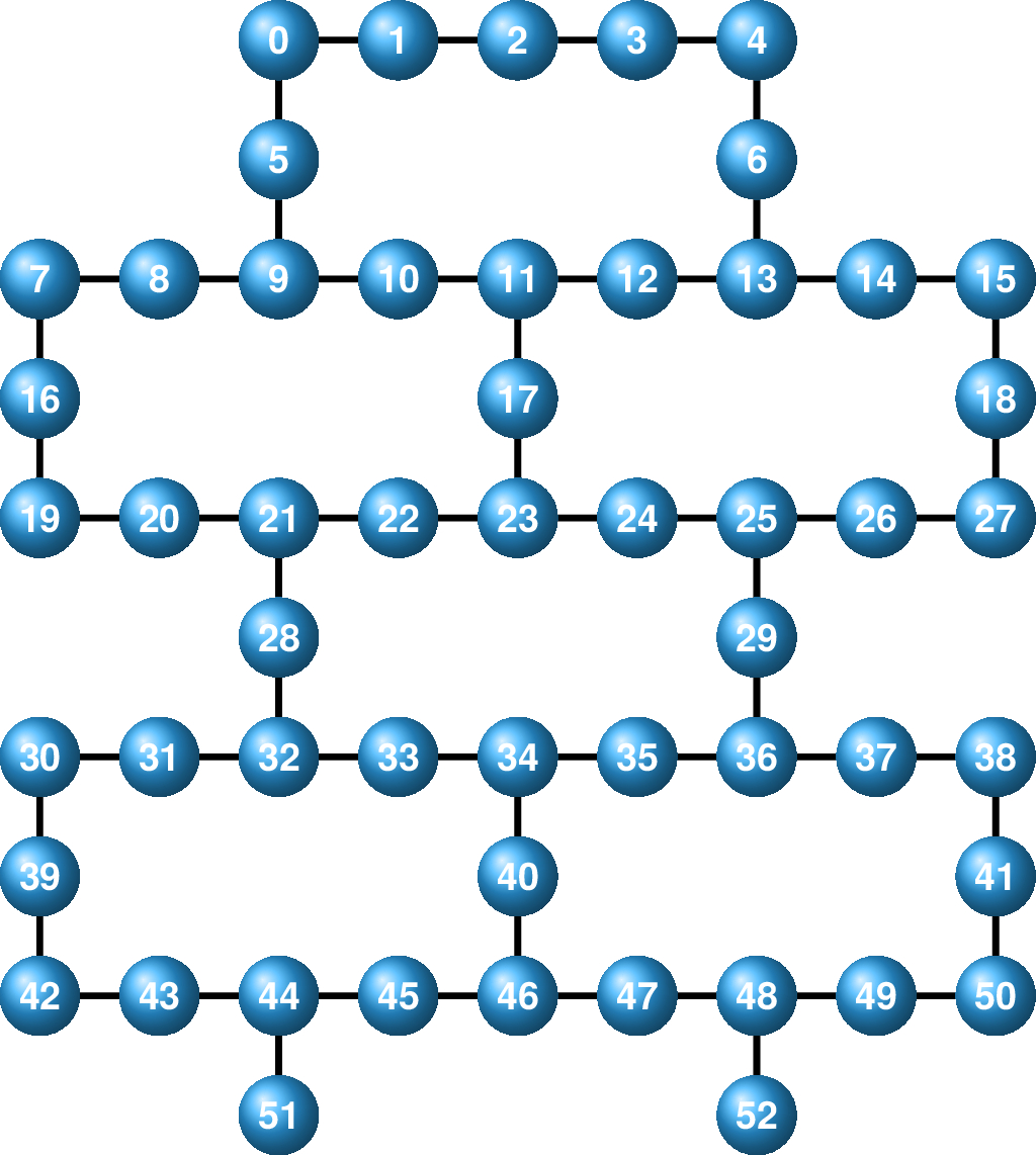
It is not necessary to physically connect every qubit with every other qubit. The chip architecture determines the degree of connectivity so that overall performance and manufacturability is optimized. For example, below is the connection map for the IBM Q first generation 20-qubit chip from 2017. [16]
Since then, the layout of the 20-qubit chip was changed to decrease the errors coming from nearby connected qubits and prepare for eventual qubit and gate error correction.

Through the entanglement, starting with the physical connections, we must be able to see and use the doubling of the C (Hilbert) vector space for every additional qubit added to the system.
Since one qubit is never enough, we should be able to add, over time, sufficient additional qubits to do useful quantum calculations. The cost to add these qubits should not be prohibitive. We would not, for example, want the economic cost or the engineering complexity to scale exponentially as we increase the number of qubits.
Initializing qubits
We must be able to initialize a qubit to a known initial state with very high probability. This is called ‘‘high fidelity state preparation.’’
Since it is common for algorithms to begin with qubits in |0⟩, this is a good choice. If |1⟩ is a better choice for the technology, applying an ![]() gate after initialization gives an equivalent effect.
gate after initialization gives an equivalent effect.
Long decoherence
As we will see in section 11.4, decoherence causes a qubit to move from a desired quantum state to something else. If too much decoherence happens, the state is random and useless.
The qubit must have a long enough coherence time so that enough quantum gates can be executed to implement an algorithm that does something useful. If you have a long coherence time but your gates take a long time to execute, that may be equivalent to a short coherence time but with fast gates.
Long coherence, fast enough gates, and low error rates will be the key to success with NISQ quantum computers.
Universal set of gates
You can’t build a house if you don’t have the right tools. You can’t build general quantum algorithms unless you have a complete-enough set of gates.
In section 9.3, we looked at how gates can be created from other, more primitive ones. The gates that are native to a particular qubit technology may not look anything like the ones we have seen in this book, but as long as they can be composed into a standard collection, practical algorithms can developed, implemented, and deployed.
Measurement capability
We must be able to reliably force the qubit into one or the other of two orthonormal basis states, and these are often |0⟩ and |1⟩. The error rate of this operation must be low enough to allow for useful computation: if we get the wrong measurement answer 50% of the time, all the previous work on executing the circuit is lost. This is called ‘‘high fidelity readout.’’
If we move the qubit to |+⟩= ![]() , it should measure to either |0⟩ or |1⟩ with 0.5 probability each. The same is true for quantum states with known probability amplitudes before measurement.
, it should measure to either |0⟩ or |1⟩ with 0.5 probability each. The same is true for quantum states with known probability amplitudes before measurement.
To learn more
In 2018, DiVincenzo published a brief retrospective on the creation of and progress in implementing quantum computers that respected his criteria. [9]
11.3 Light and photons
Light literally illuminates the things around us. It can be as dim and small as a faraway star on a clear night, or can be harsh and bright as the sun or the output of welding equipment. Understanding exactly the nature of light was a major research direction in physics in the nineteenth and early twentieth centuries.
The answers ended up being far more complicated than anyone imagined, gave birth to quantum mechanics, and involved the electromagnetic spectrum well beyond visible light.
11.3.1 Photons
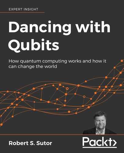
Does light behave like a wave, with varying amplitude A (height) and frequency ν? The wavelength λ is the distance between two wave crests or other corresponding points. (λ is the Greek letter ‘‘lambda’’ and ν is the Greek letter ‘‘nu’’.)

Or does light behave like a particle with a well-defined shape, shooting off in various directions? Can particles have different energies? Can particles have different colors?
Light has both wave-like and particle-like characteristics. The fundamental unit of light is called a photon. It has no charge and, according to theory, it has no mass.

A photon never sits still. The speed of light is how fast a photon moves in a vacuum. This is denoted by c and is 299,792,458 meters per second, which is approximately 186,282 miles per second.
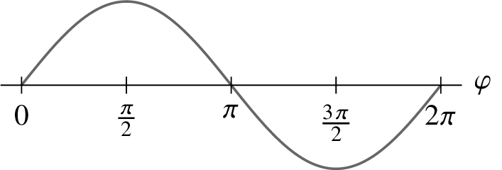
When two waves take up the same space at the same time, we get superposition, as shown on the left-hand side in the plot below.

This leads to interference, shown on the right-hand side in the plot. At any point where the waves overlap, their amplitudes, positive or negative, add to give a new combined amplitude. If both amplitudes are the same sign, we get constructive interference. If they differ, we get destructive interference. If the new amplitude is zero, we have complete destructive interference.
For a given wave with a repeating period as we have shown, we measure the various points along the horizontal from the beginning of the period to the end in radians and call this the phase ϕ. It takes on values from 0 to 2π.
When two waves have the same shape, the same amplitude, and the same frequency but are possibly offset horizontally, we say that the waves are coherent. The offset Δϕ is the phase difference or phase offset.

Note that some authors also call this phase difference ϕ, which is confusing.
Frequency is measured in hertz, Hz, which is one full cycle per second. The solid line on the left has a frequency of 1 Hz while the dotted line has a frequency of 4 Hz.
One gigahertz (GHz) is a frequency of one billion (109) cycles per second. A terahertz (THz) is 1012 cycles per second.
To finish our discussion of photons, we need to know about a fundamental value that appears to be essential to how our universe works. That is, if we vary this number, all sort of physics that exists for us would either be different or impossible. Planck’s constant, h, is an exceptionally small number and is
| h | = 6.62607004 × 10⁻³⁴ m2 kg / s |
| = 0.000000000000000000000000000000000662607004 m2 kg / s . |
Thinking a of photon as a wave, let ν be its frequency measured in Hz. Its energy E measured in Joules is
Question 11.3.1
What is the unit we used for Hz? Determine this from the units for E and ν. One Hz is equal to how many Joules?
The higher the frequency of the photon (or the smaller its wavelength), the greater its energy.
A wave that is travelling at a constant speed has wavelength λ equal to that speed divided by the frequency ν. Wavelengths are usually measured in some variation of the meter such as the nanometer, nm. One nm = 10−9 meters, or one-billionth of a meter.
Visible light is only part of the full electromagnetic spectrum. Infrared radiation, microwaves, and radio waves all have wavelengths longer than visible light, and so less energy. Ultraviolet radiation, x-rays, and gamma (γ) rays all have shorter wavelengths, hence higher frequencies, and more energy.
γ rays have frequencies above 1019 Hz and wavelengths less than 10−11 m. On the other side, microwaves have frequencies between 1 GHz and 300 GHz, and wavelengths from 0.30 m to 0.001 m. Note that the exact wavelength boundaries between different types of electromagnetic radiation vary quite a bit in books and articles, depending on which source you consult.
Coherent light is defined as above (same amplitude, same frequency) but we require that the waves are in phase with one another. Light that varies in frequency or phase is called incoherent light.
Coherent light can be produced via Light Amplification by Stimulated Emission of Radiation, which gives rise to the word ‘‘laser.’’ A laser can be focused to send a beam of photons a great distance or for cutting materials. They are also used in scanners at stores to read bar codes and, historically, to read and write data to compact discs, DVDs, and Blu-ray discs.
Question 11.3.2
Compact disc technology used light with a wavelength of 780 nm while Blu-ray used 405 nm. Where are these on the light spectrum?
11.3.2 The double-slit experiment
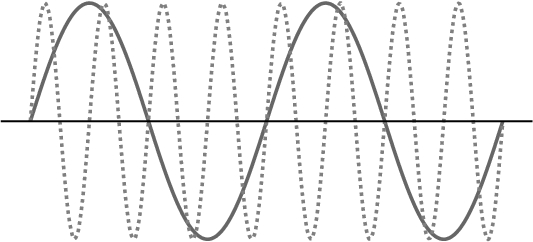
Suppose you have a device that allows you to shoot perfectly spherical pellets against a smooth, blank wall. The pellets are the same size and do not vary in their straight path or their speed once they leave the device.
We can see where each pellet struck the wall.
Now let’s insert a pellet-proof flat shield between the device and the wall. Also, we cut a horizontal slit that should allow only the center pellet to pass through.

The shield blocks all the pellets except those lined up with the slit. We can repeat this with two slits.

If we shoot many pellets and allow for some horizontal scattering, the impact area on the wall, shown in green, would look like the shape of the slit.
Instead of pellets, let’s consider photons. Our ‘‘photon shooting’’ device is a laser and so the light is coherent with some constant wavelength. Thought of as a particle, a photon passes through one slot or the other but not both. However, photons also behave as waves.
The light waves interfere with themselves after they pass through the slots. Instead of getting solid bands directly behind the slits, we get diffraction and strong bands between the slits and weakening bands to each side. This is because of constructive and destructive interference.
This ability of light to sometimes behave like a wave and sometimes behave like a particle is called the ‘‘wave-particle duality,’’ though it is considered more of a historic physical model than modern quantum optics. [11] [25]
11.3.3 Polarization
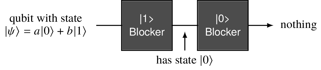
Consider a general quantum state for one qubit in the computational basis: |ψ⟩ = a |0⟩+ b |1⟩. We are going to pass the qubit through a series of procedures and see what comes out the other end.
The first is the |1⟩ blocker.

In this somewhat unnatural process, we start with a qubit in general state and pass it through the blocker. With probability |a|2 the qubit will emerge on the other side and it will have state |0⟩. With the complementary probability |b|2, the qubit will be completely blocked and nothing will emerge. Bye bye qubit.
In a similar way we can define the |0⟩ blocker.

If we compose these, no qubit makes it through.
Our final procedure is the |+⟩ blocker.

What do we get if we do this?

Recall we have these fundamental equalities among basis kets:
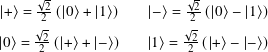
After the |1⟩ blocker, we have |0⟩ with probability |a|2, if anything. Assuming something is there, it is also equal to ![]() . We run this through the |+⟩ blocker and with probability 0.5 =
. We run this through the |+⟩ blocker and with probability 0.5 = ![]() we get |−⟩ or nothing. If anything, it is also equal to
we get |−⟩ or nothing. If anything, it is also equal to ![]() .
.
Now we pass it through the |0⟩ blocker. With probability 0.5 = ![]() we get the qubit in state |1⟩.
we get the qubit in state |1⟩.
In the case where we used only the |1⟩ and |0⟩, no qubit in any state made it through. Oddly enough, if we inserted the |+⟩ blocker between them, that qubit in initial state a |0⟩ + b |1⟩ made it through with probability |a|2 × 0.5 × 0.5 = |a|2/4.
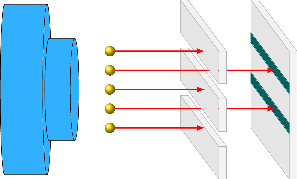
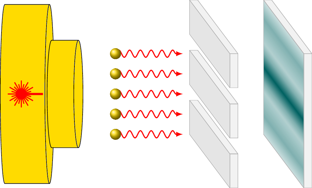
This is the mathematics behind the famous three filter polarization experiment, which I now illustrate.
When you think of a photon as a wave, the wave travels in one direction but the peaks and crests of the waves are perpendicular to the direction. Consider a string on a musical instrument. If you pluck it by pulling straight up and releasing, the wave will rise and fall vertically, or ↑. If you pluck it directly on its side, the wave will rise and fall from left to right, or horizontally (→).
A photon is a two state quantum system and we can use {|↑⟩, |→⟩} as an orthonormal basis. Rather than thinking about a qubit making it through the above blocking processes, we consider a photon passing through or being absorbed by a polarization filter. We start with a photon in the general a |↑⟩ + b |→⟩ state.
A |↑⟩ vertical polarization filter absorbs the photon with probability |a|2 and passes it through with probability |b|2. Similarly, a |→⟩ horizontal polarization filter absorbs the photon with probability |b|2 and passes it through with probability |a|2.
A |↑⟩ filter followed by a |→⟩ filter absorbs all photos. This is similar to our |1⟩ blocker followed by the |0⟩ blocker.

If we now add a middle filter for |↗⟩ in the {|↗⟩, |↘⟩} basis, the photon will reach the wall with probability |a|2/4 ({|↗⟩, |↘⟩} play the role of {|+⟩, |−⟩} from above.)

This experiment was first proposed in a 1930 textbook by Paul Dirac. [8] It demonstrates quantum states, superposition, and alternative sets of basis kets.
Question 11.3.3
Instead of having the middle filter at 45○ to the others, imagine you can rotate it from the horizontal to the vertical. How does the probability of a photon reaching the wall change? Can you express this mathematically?
To learn more
Given the polarization of light as a two-state quantum system, you might think that you might be able to use photons in the implementations of qubits. You would be correct, and this is the basis for significant academic research and several startup companies.
To see how the techniques satisfy DiVincenzo’s Criteria from section 11.2 , see the articles by Knill, O’Brien, and others. [17] [21] [22]
11.4 Decoherence
There are three important measurements that quantum computing researchers use to measure coherence time: T1, T2, and its cousin T2*. Let’s begin with T1. They are single qubit measurements and so we can use the Bloch sphere to discuss them. Their use goes back to Felix Bloch’s work on nuclear magnetic resonance (NMR) in the 1940s. [1]
11.4.1 T1
T1 goes under several names, all of them connected to the physics of various underlying quantum processes:
- relaxation time,
- thermal relaxation,
- longitudinal relaxation,
- spontaneous emission time,
- amplitude damping, and
- longitudinal coherence time.
It is related to the loss of energy as the quantum state decays from the higher energy |1⟩ state to the |0⟩ ground state. This energy is transmitted to, or leaked into, the environment and lost from the qubit. T1 is measured in seconds or some fraction thereof such as microseconds. A microsecond is one-millionth of a second, 10−6 seconds.
For the computation of T1, the qubit is moved via an X gate from |0⟩ to |1⟩. The decay toward the lower energy state |0⟩ is exponential and follows the rule
An outline of a scheme to compute T1 looks like this:

- Initialize a counter c in Z to 0. Initialize time t to 0. Initialize the number of runs per time increment to some integer n. For example, n = 1024 is reasonable. Choose some very small ε in R.
- Set the time increment between measurements to some small value Δt. (The Greek letter
 , ‘‘Delta,’’ is commonly used for the incremental difference between some value and the next.)
 - Add Δt to t.
- Initialize the qubit to |0⟩, apply X, and wait t seconds.
- Measure. If we see |1⟩, add 1 to c.
- Go back to step 4 and repeat n − 1 times. If we have done this already, go to the next step.
- Compute pt = c/n as the percentage of times we have seen |1⟩.
- Save and plot the data (t, pt).
- Reset c to 0, go back to step 3 and repeat until pt < ε.
The decay of the quantum states for two qubits q1 and q2 is shown in this graph:

T1 is the value of t when pt = 1/e ≈ 0.368. In this example, q2 has a larger T1 and so has a larger longitudinal coherence time.
It’s interesting to ask at this point when my qubit is in state |0⟩ due to the decay. That is, if we wait long enough after T1 will the qubit have gone completely to the lower energy state? Theoretically, it is just getting asymptotically closer and the probability of seeing |0⟩ is increasing to 0.9999+.
In practice, if you want the qubit back in an initial |0⟩ state, you wait a time which is a few integer multiple of T1. You now either assume that statistically you are at |0⟩ or you do a measurement. If you get |0⟩, you are done. If you get |1⟩, apply an X.
This last step depends on your ability to do such a conditional action in your hardware and control software. If you can do it, you don’t have to wait past T1, you can just measure and conditionally move to |0⟩ when you wish. See, for example, the |0⟩ reset operation in subsection 7.6.13.
Given
11.4.2 T2 and T2*
If T1 concerned itself with going from the south pole to the north, T2 adds in the extra element of what is happening at the equator. As a reminder, when I say ‘‘the equator,’’ I mean the intersection of the xy-plane with the Bloch sphere.
Like T1, T2 and its related metric T2* go by several names:
- dephasing time,
- elastic scattering time,
- phase coherence time,
- phase damping, and
- transverse coherence time.
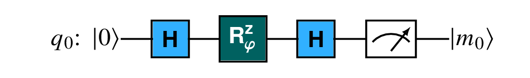
In a perfect world, the circuit

would return |0⟩ with a probability of 1.0 every time. Though it does nothing in the logical circuit, think of the ID as a point in the circuit where we might wait a short period of time before doing the final H.
The circuit should bring us from |0⟩ to |+⟩ and back to |0⟩. We move to the equator and then go back to |0⟩. Note that neither |0⟩ nor |1⟩ has a phase component, so we need to experiment elsewhere and the equator is the obvious choice.
This doesn’t happen with a physical qubit. Instead, once we move to the equator we begin drifting a little around the xy-plane.
In this example on the Bloch sphere, once we get to |+⟩ we move counterclockwise by some small angle ϕ in some small time increment. That is, the qubit state is not stable.

We also expect the state to be moving toward lower energy but I am focusing on what is happening with the phase. Similarly, when we look at T1, there can be phase drift but we are looking the longitudinal decoherence.
This is an idealized and simplified version of the circuit where we see only the phase shift:
Consider the matrix version:
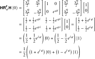
When ϕ = 0 we get |0⟩, as expected. When ϕ = π, ![]() =
= ![]() = Z, and the result is |1⟩. When 0 < ϕ < π, the two probability amplitudes are non-zero.
= Z, and the result is |1⟩. When 0 < ϕ < π, the two probability amplitudes are non-zero.
In particular, the amplitude of |0⟩ is

If the phase change continued at a constant rate over time, you might expect the graph to look like this:

Instead, there is decay toward a probability of 0.5 but with the same short-term periodic behavior.

It is only short term because eventually the quantum state will fully decay to |0⟩ and the final H will place the state on the equator. At that point the probability of getting |0⟩ is exactly 0.5.
The measurement here is called T2* and the circuit is a Ramsey experiment. We are considering the wait time between the H gates. During this time some rotation ϕ around the z-axis occurs.
I want to emphasize again that what I have shown here assumed only one kind of noise, the phase drift, and even that was constant. In a real qubit, other noise and irregularities will affect the coherence, including longitudinal decoherence.
Moreover, by using ![]() to illustrate the phase drift, I’ve given the impression that the noise looks like a nice unitary transformation. It does not, as we see in the next section.
to illustrate the phase drift, I’ve given the impression that the noise looks like a nice unitary transformation. It does not, as we see in the next section.
The high-level scheme to measure T2* is:
- Initialize a counter c in Z to 0. Initialize time t to 0. Initialize the number of runs per time increment to some integer n. For example, n = 1024 is reasonable. Choose some very small ε in R.
- Set the time increment between measurements to some small value Δt.
- Add Δt to t.
- Initialize the qubit to |0⟩, apply H, and wait t seconds. Apply H again.
- Measure. If we see |1⟩, add 1 to c.
- Go back to step 4 and repeat n − 1 times. If we have done this already, go to the next step.
- Compute pt = c/n as the percentage of times we have seen |1⟩.
- Save and plot the data (t, pt).
- Reset c to 0, go back to step 3 and repeat until 0.5 − ε < pt < 0.5 + ε.
For small enough Δt, T2* is the largest time t where pt ≤ 1/e.
A related metric called T2 is gotten via a Hahn Echo with a similar circuit.

The difference from T2* is that instead of waiting the full time t before the final H, we wait half that long, do an X, wait the remaining time, and then conclude with the H and measurement. By doing this we are canceling some of the phase drift but keeping the effects of other noise. This technique is called ‘‘refocusing.’’ [15]
Generally, T2* ≤ T2 ≤ 2 T1. [29]
11.4.3 Pure versus mixed states
Each of the quantum states we have considered so far is a pure state. These are single linear combinations of basis kets where the probability amplitudes are complex numbers. The sum of the squares of their absolute values add up to 1. Each such square of an absolute value is the probability that we will see the corresponding basis ket when we measure.
There are times when we need to represent a collection, an ensemble, of pure states in which our qubit register may reside. This is different from a superposition where we are looking at a quantum phenomenon related to the complex coefficients of the basis kets.
If {|ψ⟩1, |ψ⟩2, …, |ψ⟩k} is a collection of pure quantum register states, we define a mixed state as
The density matrix of a mixed state is the sum of the density matrix of the pure states weighted by the pj. If ρj = |ψj⟩⟨ψj| is the density matrix of a pure state in the ensemble, then
A density matrix ρ corresponds to a pure state if and only if tr (ρ2) = 1. Otherwise, tr (ρ2) < 1 and we have a non-trivial mixed state.

Question 11.4.1
Prove algebraically that 2p2 − 2p + 1 < 1 when 0 < p < 1.
11.5 Error correction
In section 2.1 and section 6.4 we looked at some of the basic ideas around classical repetition codes: if you want to send information, create multiple copies of it and hope that enough of them get through unscathed so that you can determine exactly what was sent.
For the quantum situation, the No-Cloning Theorem (subsection 9.3.3) says that we can’t copy the state of a qubit, and so traditional repetition is not available.
What we can do is entanglement, and it turns out that this is powerful enough when combined with aspects of traditional error correction to give us quantum error correction, or QEC.

How can we go from |ψ⟩ = a |0⟩ + b |1⟩ to a |000⟩ + b |111⟩? As you start thinking about such questions, there are two good starting points: ‘‘would applying an H change the situation into something I know how to handle,’’ and ‘‘how might a CNOT and entanglement affect things?’’
Since I already let on that entanglement is part of the solution, note that a simple
takes |ψ⟩|0⟩|0⟩ to a |000⟩ + b |111⟩. Each CNOT changes the |0⟩ in q1 and q2 to |1⟩ if the amplitude b of |1⟩ in |ψ⟩ is non-zero. Similarly, the CNOT does nothing if the amplitude a of |0⟩ in |ψ⟩ is non-zero.
Given this, how can we fix bit flips?
11.5.1 Correcting bit flips
In the classical case of a bit, only one thing can go wrong: the value changes from 0 to 1 or vice versa. Of course, noise may cause multiple bits to change, but for one bit there is only one kind of error.
In the quantum case, a bit flip interchanges |0⟩ and |1⟩ so that a general state a |0⟩ + b |1⟩ becomes a |1⟩ + b |0⟩ instead. From subsection 7.6.1, this is what an X does, but when we are thinking about noise and errors, we are saying that a bit flip might happen, not that it definitely does.
If we absolutely knew that an X was applied, we could just do another one and fix the problem. Therefore we need to get more clever. Consider the circuit

We start the analysis by looking at the possible quantum states at each numbered vertical line. We begin with |ψ⟩ = |0⟩.
| Step 1 | Step 2 | Step 3 | Step 4 | Step 5 | |
| No errors | |||||
| One error | |||||
| Two errors | |||||
| Three errors |
Question 11.5.1
Create the table for |ψ⟩ = |1⟩.
Question 11.5.2
What is the role of the Toffoli gate between vertical lines 4 and 5?
This circuit corrects up to one bit flip error in q0. When the error is not corrected, the result of the circuit is always a bit flip in q0.
If the probability of getting a bit flip error is p, the probability of no error is 1 − p. We previously worked through the full probability of our being able to fix at most a single error in section 6.4 .
11.5.2 Correcting sign flips
A sign flip is a π phase error that switches a |0⟩ + b |1⟩ and a |0⟩ − b |1⟩. As we saw in subsection 7.6.2 , a Z gate does this.
Changing between the usual computation basis of |0⟩ and |1⟩ and the Hadamard basis of |+⟩ and |−⟩ has the extremely useful property of interchanging bit flips and sign flips. To fix possible sign flips, we only have to insert some H gates into the above circuit. This is a consequence of H X H = Z and the equivalent H Z H = X.

Can we combine these ideas to fix at most one bit, a sign flip, or both? This would be equivalent to fixing an errant X, Z, or Y gate.
11.5.3 The 9-qubit Shor code
To correct either one sign flip or one bit flip, we need eight additional qubits beyond the qubit we are trying to maintain. The circuit in Figure 11.1 is based on work published in 1995 by Peter Shor, the same year he published his breakthrough factoring paper. [27]

As we saw earlier, any 2 by 2 unitary matrix can be written as a complex unit times a linear combination of I2 and the three Pauli matrices. I2, σx, σy, and σz are the matrices for the ID, X, Y, and Z, respectively. Since we can repair a single error for these gates (where ID is really no error), we can repair any single error that is a linear combination of them.
The Shor 9-bit code can correct any single qubit error corresponding to a unitary gate.
If we have n qubits then we can use 9n qubits to duplicate the above circuit n times. The best error correcting code that can correct like the Shor code uses only 5 qubits, and this is as good as is possible. [18]
What happens if an error occurs in one of the CNOT or Toffoli gates in the circuit?
11.5.4 Considerations for general fault tolerance
It appears we have a problem: to correct errors we need more qubits, and then we need more qubits to correct the error correcting qubits, and so on. Does it ever stop?
Yes, but we need to use different methods such as surface codes based on group theory and a branch of mathematics called topology. In essence, if we can get the error rates of our qubits and gates close to a certain threshold, then we can use entanglement and a lot of qubits to give us fault tolerance. We especially need our two-qubit gate fidelities to improve since those are usually much worse than for single gates.
How many? At the 2019 error rates of the best quantum computing systems, we need approximately 1000 physical qubits to create one logical qubit. Also at this time, the largest working quantum computers have 53 or 54 qubits. More pessimistic estimates put the number of physical qubits we need close to 10,000.
One logical qubit does not do anyone much good. We’ll need hundreds and thousands of these for the most advanced applications people foresee for quantum computers. For example, for Shor’s algorithm to factor a 2048 bit number, somewhere around 100 million = 108 physical qubits may be needed. This translates to 105 = 100,000 logical qubits.
Other than being used in computation, fault-tolerant qubit technology might also be used for quantum memory and storage. Note, however, there is a twist to this. Unlike in classical computing where you can copy data from memory into a working register for use, you cannot copy a qubit per the No Cloning Theorem from subsection 9.3.3.
But you can use teleportation (subsection 9.3.4 )! It’s very strange indeed to imagine a computing system with teleportation but no data replication.
I believe that error correction will be introduced partially and incrementally. As we become better able to build quantum devices with lower qubit and gate error rates, we’ll be able to perform some degree of limited error correction, so as to at least extend coherence times for some qubits. This will allow us to intelligently use these and the remaining raw physical qubits to implement algorithms that may not look quite so clean and elegant as what we saw in chapter 9 and chapter 10.
By ‘‘us’’ I really mean ‘‘our optimizing compilers.’’ As the architecture of quantum devices gets more sophisticated, we need compilers to smartly map our quantum application code in an optimal way to the number and kinds of qubits and available circuit depths.
The formal description of single-qubit errors is in terms of density matrices, mixed states, and probabilities and gives rise to the same for two qubits and the gates that operate upon them. This is then part of the machinery that has given rise to the theory of large-scale quantum error correction and, we hope, its eventual implementation. [20, Chapter 8]
To learn more
For an overview of error correction techniques and to see early qubit estimates for implementing Shor’s algorithm, see Fowler et al. [12] Over time, calculations for such estimates tighten up and improve.
Now that you have almost finished this book, you can read a ‘‘beginners guide’’ to error correction. [7] There is significant current research on error correction and potential hardware implementations. [3] and [14]
11.6 Quantum Volume
How powerful is a gate- and circuit-based quantum computer? How much progress is being made with one qubit technology versus another? When we say we can find a solution on a ‘‘powerful enough’’ quantum computer, what does that mean? When will we know we have arrived?
While it is certainly useful to know how well a given qubit is doing in terms of decoherence and error rates, it tells you nothing about the system in total and how well the components are working together. You may have one or two spectacular, connected, and low error rate qubits, but other aspects of your system may make it unusable for executing useful algorithms.
Implementing hundreds of very bad qubits does not give you an advantage in the circuit model over having far fewer but excellent qubits with good control and measurement. Therefore, we need a whole-system, or ‘‘holistic,’’ metric that can tell us at a glance the relative of our quantum computer.
Such an architecture-independent metric is called Quantum Volume and was devised by scientists at IBM Research in 2017. [6]
Quantum Volume is reported as 2v where the best performance of your system is seen on a test circuit area v qubits wide by v gates deep. In 2019, IBM announced that it had reached a Quantum Volume of 16 = 24 for its superconducting transmon quantum computing systems and expected to be able to at least double it year over year for the next decade. [13]
Though IBM came up with this metric, there is nothing brand-specific about it. Indeed, other researchers have proposed generalizations of the metric to decouple the width and depth of the circuits being tested. [2]
The range of factors taken into account by Quantum Volume include
-
calibration errors
How well the electronic controls for programming and measuring qubits are calibrated to ensure accurate operation and error mitigation.
-
circuit optimization
How well an optimizing compiler improves the layout and performance of a circuit across its depth and qubit register width.
-
coherence
How long the qubit stays in a usable state as discussed in section 11.4 .
-
connectivity and coupling map
How qubits are connected to other qubits and in what patterns.
-
crosstalk
How the state of one qubit affects nearby qubits, either in gate operations or through more passive entanglement.
-
gate fidelity
At what error rates do gate operations move qubits from their current to new states.
-
gate parallelism
How many gate operations can be run on qubits in parallel, that is, at the same time. This is different from the concept of quantum parallelism.
-
initialization fidelity
How accurately we can set the initial qubit state to something known, usually |0⟩.
-
measurement fidelity
How accurately we can collapse a qubit state and read it out as |0⟩ or |1⟩.
-
number of qubits
More can be better, but not always. In any case, you need a sufficient number.
-
spectator errors
How much is a qubit that is supposed to be idle affected during a 1- or 2-qubit gate operation on a physically connected qubit.
As a metric, gate fidelity varies between 0.0 and 1.0, inclusively. A value of 1.0 says the gate perfectly implements the intended logical unitary transformation. Two-qubit gates typically have gate error rates much higher than single qubit gates, on the order of ten times worse.
Having qubits connected to more qubits can be a good thing, as long as that coupling does not introduce additional errors across the connected qubits.
This is one of the reasons why Quantum Volume will not increase solely by adding more and increasingly coupled qubits.
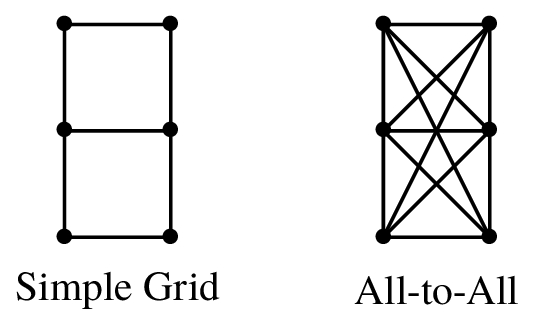
Where a quantum device is laid out in a physical medium like silicon, it can use non-square and non-rectangular patterns. Regular polygonal tiling patterns can be used, with the qubits not necessarily at the corners. Moreover, patterns can vary in different regions of the device and along the edges.
Question 11.6.1
In Figure 11.2, what’s the maximum number of qubits to which one qubit is connected? Minimum? What is the average number of qubits to which each qubit is connected? [19]
Having a well-performing optimizing compiler can increase Quantum Volume by reducing the number of gates and rearranging how and when they are applied to qubits. By avoiding qubits with shorter coherence times and greater one- and two-qubit error rates, and using native gates on well connected qubits, quantum volume may be increased significantly by the compiler.
The theory and implementation of optimizing compilers for classical computers is well known and has been studied over decades. Quantum ‘‘transpiling’’ (transformational compiling) is in its infancy but fast progress is already being seen in Qiskit through the open source community of computer scientists, quantum researchers, and software developers from academia and industry.
The number of qubits is a very bad and inaccurate metric of the quality and performance of a quantum computer. Rather, use Quantum Volume to get a whole-system measure of what your hardware, software, system, and tools for software development can do.
11.7 The software stack and access
One way of accessing a quantum computing system looks like this:
- You have downloaded and installed software development tools like the Qiskit open source quantum computing framework to your laptop or workstation. [24]
- You develop your quantum code in a programmer’s editor or a JupyterTM notebook. [23]

- When run, part of your application connects to a quantum simulator on your computer or remotely to real quantum hardware or a simulator.
- The remote connection is via the Internet/cloud.
- Your application invokes one or more processes that runs on the quantum hardware or a simulator.
- Ultimately, your application makes use of the results of the quantum computation and does something valuable within your use case.
There are at least two other similar scenarios:
- Instead of developing locally, you do so via a web browser-based environment where your Jupyter notebooks are edited, tested, stored, and executed on the cloud.
- You have runnable code that you place in a container in the cloud and it accesses quantum computers either close to or remote from the classical cloud servers.
For developers, the software stack looks like the diagram above. On the bottom is the System level and this can include APIs for hooking in higher-level services and benchmarking.
The Pulse level, for quantum computing systems that use microwave control systems, allows direct definition and use of the microwave pulses that configure quantum gates.
Above that is the support for using builtin gates and creating new circuits. This allows implementing them within quantum registers and building out the algorithms we discussed in chapter 7 through chapter 10 .

At the System Libraries level, the coder can re-use previously defined and optimized circuits within their own circuits or application code. When using these libraries, the developer mindset is still in terms of how quantum algorithms work but is well above anything that could be described as ‘‘assembly language.’’
Finally, at the User Libraries level we have convenience libraries to accelerate general software development. Here a developer might not even be aware that a quantum computing system is used at all.
This stack representation gives you a rough idea of where functionality is provided from deep down and close to the quantum computer all the way to the most abstract access points. Any particular framework may structure its developer software stack in more or fewer levels.
Before we leave this topic I want to give my opinion on whether we need new programming languages just for quantum computing or if the functionality should be embedded within existing languages. For various scientific applications in the past, I’ve done both.
For many of us, it’s fun to create new languages. That might not be your idea of fun, but so be it! It’s very tempting to start building a quantum programming environment and then find you are spending too much time doing classical computer science engineering, most of which has likely been done before – and better.
Modern programming languages like Python, Swift, Go, Java, and C++ are superb for software development. For me, it makes much more sense to build the quantum gate, circuit, and execution support within the type systems of these kinds of languages. In this way, you can quickly use the entire tool chain and support for the established languages and concentrate on quickly and comprehensively adding quantum software development.
Moreover, if your development framework is open source, you have a much larger potential set of contributors who know the existing languages than if you need to teach them a new one.
As an example, Qiskit uses Python as the main developer language but provides extensive libraries at all levels of the software stack. In some cases, lower-level access or optimized code was written and then provided with Python library interfaces.
11.8 Simulation
Is it possible to simulate a quantum computer on a classical computer? If we could do it, ‘‘quantum computing’’ would be only another technique for coding software on our current machines.
In this section we look at what you have to take into account if you want to write a simulator for manipulating logical qubits.
If you have a simulator handy, such as one that is provided by Qiskit or the IBM Q Experience, you can use it for small problems. Here we look at how you might build a simulator, in general terms. I offer no complete code in any particular programming language but more of a list of what you need to take into account. You can skip this section if you are not interested in such concerns.
11.8.1 Qubits
Your first decision when thinking about building a quantum computing simulator is how you represent qubits. With this and your other choices, you can build a general model or you can specialize it. We’re going for the general case. Once you complete this section you can go back and think about how each of the interconnected parts can be optimized individually and together.
We want to work with more than one qubit and so we do not use a Bloch sphere. The state of a qubit is held in two complex numbers and you can store them in an ordered list, array, or similar structure. If your language or environment has a mathematical vector type, use it.
While we might here use an exact value like
If you have an n-bit quantum register, you need to represent a vector of 2n complex numbers. If n = 10 then a list of 1024 complex numbers uses 9024 bytes. For 20 qubits it is 8,697,464 bytes or approximately 8.3MB. Just adding two more qubits brings this to 35,746,776, or 34MB.
Think about this: for a single state of a quantum register with 22 qubits you need 34MB to represent it. It gets exponentially bigger and worse than this as we add more qubits. We are over a gigabyte per state at 27 qubits. It’s not only storage that is increasing, the time required to manipulate all those values is getting big fast. Your choice of algorithms at every level is critical.
It gets even worse: the size of the matrix for a gate is the square of the number of entries in the qubit state ket.
With optimizations we can get these numbers lower but the exponential nature of growth will eventually catch up with you. You might be able to do a few more qubits but simulation will eventually run out of steam. One way of doing this is to use single precision floating point numbers instead of double. It saves memory, briefly.
My guess is general-purpose quantum computation simulation will get too big and time-impractical even for supercomputers somewhere in the mid-40 number of qubits. If you have a very specific problem you are trying to simulate, then you may be able to simplify the mathematical formulas that represent the circuit. Just as sin2(x) + cos2(x) reduces to the much simpler 1, the math for your circuit may get smaller. Even then I think it is likely that special purpose simulation will top out around 70 to 80 qubits.
Simulation is good for experimentation, education, and debugging part of a quantum circuit. Once we have powerful and useful real quantum computers of more than 50 qubits or so, the need for simulators will decline, probably along with the commercial market for them, too.
Consider using a sparse representation for qubits and ket vectors. Do you really need 250 = 1,125,899,906,842,624 numbers to represent the state |0⟩⊗ 50? After all, there are only two pieces of significant information there, 0 and 50. Add a little overhead for representing the sparse ket and you can fit it all into a few bytes.
11.8.2 Gates
If qubits are vectors, then gates are matrices. The most straightforward way of implementing multi-wire circuits is to construct the tensor product matrix for two gates. These matrices get quite large: if you have n qubits then your matrices will be 2n by 2n in size.
For the subcircuit

we have the product of the matrices corresponding to ID ⊗ H


11.8.3 Measurement
Once you come up with a final quantum register state like
| 0.3872983346207417 i |00⟩ − 0.6082762530298219 |01⟩ − | |
| 0.5099019513592785 |10⟩ + 0.469041575982343 i |11⟩, |
Compute the probabilities corresponding to each standard basis ket: if
example_probabilities we use in Listing 6.1 . In the output
Results for 1000000 simulated samples

Event     Actual Probability     Simulated Probability
    0              0.15                    0.1507
    1              0.37                    0.3699
    2              0.26                    0.2592
    3              0.22                    0.2202
E0 = ![]() , E1 =
, E1 = ![]() , and so on.
, and so on.
As another example, we can look at simulated measurements for a balanced superposition of four qubits. In this case, each of the amplitudes is 0.25 and its probability is 0.0625. Here is a sample run of 1000000 iterations:
example_probabilities = [1.0/16 for _ in range(16)]

Results for 1000000 simulated samples

Event     Actual Probability     Simulated Probability
    0              0.0625                    0.0627
    1              0.0625                    0.0628
    2              0.0625                    0.0627
    3              0.0625                    0.0619
    4              0.0625                    0.0622
    5              0.0625                    0.0624
    6              0.0625                    0.0624
    7              0.0625                    0.0626
    8              0.0625                    0.0622
    9              0.0625                    0.0624
    10             0.0625                    0.0624
    11             0.0625                    0.0626
    12             0.0625                    0.0631
    13             0.0625                    0.0623
    14             0.0625                    0.0625
    15             0.0625                    0.0628
Again recall, for example, that getting E7 means we are getting a result of ![]() on measurement.
on measurement.
11.8.4 Circuits
To simulate a circuit, you need to represent it in some way. Think about the wire model and then the horizontal steps from left to right where you place and execute gates.
Multi-qubit gates span wires, so you need to specify wire inputs and outputs. You need to do error checking along the way to ensure two gates in the same step do not involve the same input and output wires.
I recommend that you start with an API, an application programming interface to a collection of software routines that sits on top of your internal circuit representation. If you start by developing a new language in which to write circuits, you’ll likely spend more early coding cycles on the language rather than the simulator itself.
11.8.5 Coding a simulator
Should you decide to code a quantum simulator, here is some advice:
- Unless you want to do it as an educational project or you have a brilliant new idea, don’t bother. There are plenty of simulators out there, many of them open source such as those in Qiskit.
- Don’t start by optimizing circuits. It can be difficult enough to debug code that is supposed to do the sequence of operations you wish.
- When you do start optimizing, look for the easy stuff like getting rid of consecutive gates that do nothing. Three examples of this are H H, X X, and Z Z.
- Don’t start tensoring matrices together until you have a wire-spanning operation like CNOT.
- Build efficient subroutines that simulate standard gate combinations. Do not, for example, build a CNOT from a Toffoli gate but do provide the Toffoli gate in your collection.
- Go much deeper into how quantum gates are designed from more primitive gates. Learn about Clifford gates and how to simulate them, for example. Note, this will require deeper knowledge of quantum computing and computer science. [4] [5]
To learn more
To re-emphasize my point about not necessarily coding your own, a web search of ‘‘list of quantum simulators’’ will turn up dozens of simulators in multiple programming languages, many of them open source.
11.9 The cat
In this section we look at a well known discussion from the 1930s. We’ll use it to show an example of simulating quantum physics with quantum computing.
In 1935, physicist Erwin Schrödinger proposed a thought experiment that would spawn close to a century of deep scientific and philosophical thought, as well as many bad jokes. Thought experiments are common among mathematicians and scientists.
The basic premise is that the idea is not something you would really do, but something you want to think through to understand the implications and consequences.
This was his attempt to show how the Copenhagen interpretation promoted by Niels Bohr and Werner Heisenberg in the late 1920s could lead to a ridiculous conclusion for large objects. This is one of the popular theories for how and why quantum mechanics works, though there are others.

Niels Bohr in 1922. Photo is in the public domain.
By ‘‘large’’ here I mean ‘‘large as a cat.’’
Question 11.9.1
What does Copenhagen have to do with quantum mechanics?
The setup
In a large steel box that contains more than enough air for a cat to breathe for several hours, we place a small amount of radioactive material that has a 0.5 probability of having a single atom decay and emitting a particle per hour.
We also add a device that is a Geiger counter that can detect that single emission, plus a connected hammer that can smash open a closed vial of cyanide poison. If the Geiger counter detects anything, the hammer swings and the cyanide is released into the air.
We now place the otherwise charming but confused-looking cat into the box and seal the top.
Feel free to replace the cat with something else that would not survive in the presence of cyanide.
The wait
While we let time go by, we wonder about the state of the cat. Is he doing well or has he cast off his mortal coil? Has the radioactive emission occurred and triggered the hammer?
Until we look, we don’t know. As far as our knowledge goes, the cat is in a superposition of being dead and alive. By our opening the top, by our observing what has happened in the box, we have caused the superposition to collapse to |dead⟩ = |0⟩ or |alive⟩ = |1⟩. This is according to the Copenhagen interpretation.
In the Many Worlds interpretation, two realities were created when the opportunity for a choice was created. In one world the cat is dead, in the other it is not.
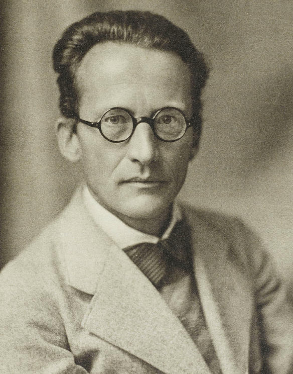
Erwin Schrödinger in 1933. Photo is in the public domain.
Now let’s express this situation in the language of a quantum circuit.
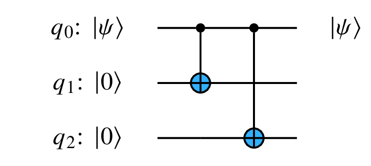
A circuit
Consider this simple circuit with two CNOT gates:
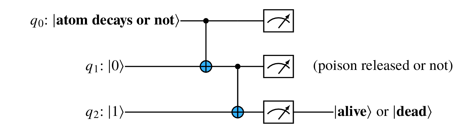
For q0, an input state of |0⟩ means no atom decays at the time the circuit is run, while |1⟩ means that a particle is emitted.
q1 is set to an initial state of |0⟩ but is flipped to |1⟩ if an atom decays. This causes the hammer to break the vial and the cyanide to enter the air.
For q2, the cat starts out in |alive⟩ = |1⟩. The final state of the cat only switches to |dead⟩ = |0⟩ if the poison is released.
Question 11.9.2
Experiment with Bell states to introduce entanglement. Do you learn anything new about the components of this experiment?
11.10 Summary
In this chapter we connected the ‘‘logical’’ idea of qubits and circuits with the ‘‘physical’’ idea of how you might build a quantum computer. We looked at the polarization of light to show a physical quantum system, and used our ket notation to understand the unusual effect we observe when using three filters. Through this we could see that the theory of quantum mechanics does seem to provide a good model for what we experimentally observe, at least in this case.
Real qubits don’t survive forever and decoherence explains the several ways in which quantum states wander over time. While we do not yet have large enough systems to implement fault tolerance, we examined what error correction might be able to do in the quantum realm.
We need to be able to measure the progress we are making and answer questions like ‘‘how powerful is your quantum computer?’’. The definition of quantum volume looks at many factors that can affect performance.
We mentioned several technologies that researchers are exploring to implement qubits. Superconducting transmon qubits are used by IBM, Google, and others, but ion traps and photonic techniques also hold promise, according to their proponent scientists and engineers.
Our cat-in-box was translated into quantum terms and got its own circuit.
References
- [1]
-
F. Bloch. ‘‘Nuclear Induction’’. In: Physical Review 70 (7-8 Oct. 1946), pp. 460–474.
- [2]
-
Robin Blume-Kohout and Kevin C. Young. A volumetric framework for quantum computer benchmarks. url: https://arxiv.org/abs/1904.05546.
- [3]
-
H. Bombin and M. A. Martin-Delgado. ‘‘Optimal resources for topological two-dimensional stabilizer codes: Comparative study’’. In: Physical Review A 76 (1 July 2007), p. 012305.
- [4]
-
S. Bravyi and D. Gosset. ‘‘Improved Classical Simulation of Quantum Circuits Dominated by Clifford Gates’’. In: Physical Review Letters 116.25, 250501 (June 2016), p. 250501.
- [5]
-
S. Bravyi et al. ‘‘Simulation of quantum circuits by low-rank stabilizer decompositions’’. In: (July 2018).
- [6]
-
Andrew Cross et al. Validating quantum computers using randomized model circuits. Nov. 2018. url: https://arxiv.org/abs/1811.12926.
- [7]
-
Simon J. Devitt, William J. Munro, and Kae Nemoto. ‘‘Quantum error correction for beginners’’. In: Reports on Progress in Physics 76.7, 076001 (July 2013), p. 076001.
- [8]
-
P. A. M. Dirac. The Principles of Quantum Mechanics. Clarendon Press, 1930.
- [9]
-
David P DiVincenzo. Looking back at the DiVincenzo criteria. 2018. url: https://blog.qutech.nl/index.php/2018/02/22/looking-back-at-the-divincenzo-criteria/.
- [10]
-
David P DiVincenzo. ‘‘The physical implementation of quantum computation’’. In: Fortschritte der Physik 48.9-11 (2000), pp. 771–783.
- [11]
-
Richard P. Feynman. QED: The Strange Theory of Light and Matter. Princeton Science Library 33. Princeton University Press, 2014.
- [12]
-
Austin G. Fowler et al. ‘‘Surface codes: Towards practical large-scale quantum computation’’. In: Phys. Rev. A 86 (3 Sept. 2012), p. 032324.
- [13]
-
Jay Gambetta and Sarah Sheldon. Cramming More Power into a Quantum Device. 2019. url: https://www.ibm.com/blogs/research/2019/03/power-quantum-device/.
- [14]
-
Jay M. Gambetta, Jerry M. Chow, and Matthias Steffen. ‘‘Building logical qubits in a superconducting quantum computing system’’. In: npj Quantum Information 3.1 (2017).
- [15]
-
Gambetta, Jay M. (question answered by). What’s the Difference between
 and
and  ? url: https://quantumcomputing.stackexchange.com/questions/2432/whats-the-difference-between-t2-and-t2.
 - [16]
-
IBM. 20 & 50 Qubit Arrays. 2017. url: https://www-03.ibm.com/press/us/en/photo/53377.wss.
- [17]
-
E. Knill, R. Laflamme, and G. J. Milburn. ‘‘A scheme for efficient quantum computation with linear optics’’. In: Nature 409.6816 (2001), pp. 46–52.
- [18]
-
Raymond Laflamme et al. ‘‘Perfect Quantum Error Correcting Code’’. In: Physical Review Letters 77 (1 July 1996), pp. 198–201.
- [19]
-
Doug McClure. Quantum computation center opens. 2019. url: https://www.ibm.com/blogs/research/2019/09/quantum-computation-center/.
- [20]
-
Michael A. Nielsen and Isaac L. Chuang. Quantum Computation and Quantum Information. 10th ed. Cambridge University Press, 2011.
- [21]
-
Jeremy L. O’Brien. ‘‘Optical Quantum Computing’’. In: Science 318.5856 (2007), pp. 1567–1570.
- [22]
-
Jeremy L. O’Brien, Akira Furusawa, and Jelena Vučković. ‘‘Photonic quantum technologies’’. In: Nature Photonics 12.3 (2009), pp. 687–695.
- [23]
-
Project Jupyter. Project Jupyter. url: https://jupyter.org/.
- [24]
-
Qiskit.org. Qiskit: An Open-source Framework for Quantum Computing. url: https://qiskit.org/documentation/.
- [25]
-
A.I.M. Rae. Quantum physics: Illusion or reality? 2nd ed. Canto Classics. Cambridge University Press, Mar. 2012.
- [26]
-
Erwin Schrödinger. What is Life? The Physical Aspect of the Living Cell. Cambridge University Press, 1944.
- [27]
-
Peter W. Shor. ‘‘Scheme for reducing decoherence in quantum computer memory’’. In: Physical Review A 52 (4 Oct. 1995), R2493–R2496.
- [28]
-
SymPy Development Team. SymPy symbolic mathematics library. 2018. url: https://www.sympy.org/en/index.html.
- [29]
-
X. R. Wang, Y. S. Zheng, and Sun Yin. ‘‘Spin relaxation and decoherence of two-level systems’’. In: Physical Review B 72 (12 Sept. 2005), p. 121303.