2
They’re Not Old, They’re Classics
No simplicity of mind, no obscurity of station, can escape the universal duty of questioning all that we believe.
William Kingdon Clifford
When introducing quantum computing, it’s easy to say ‘‘It’s completely different from classical computing in every way!’’ Well that’s fine, but to what exactly are you comparing it?
We start things off by looking at what a classical computer is and how it works to solve problems. This sets us up to later show how quantum computing replaces even the most basic classical operations with ones involving qubits, superposition, and entanglement.
Topics covered in this chapter
2.2 The power of two
2.3 True or false?
2.4 Logic circuits
2.5 Addition, logically
2.6 Algorithmically speaking
2.7 Growth, exponential and otherwise
2.8 How hard can that be?
2.8.1 Sorting
2.8.2 Searching
2.9 Summary
2.1 What’s inside a computer?
If I were to buy a laptop today, I would need to think about the following kinds of hardware options:
- size and weight of the machine
- quality of the display
- processor and its speed
- memory and storage capacity
Three years ago I built a desktop gaming PC. I had to purchase and assemble and connect:
- the case
- power supply
- motherboard
- processor
- internal memory
- video card with a graphics processing unit (GPU) and memory
- internal hard drive and solid state storage
- internal Blu-ray drive
- wireless network USB device
- display
- speakers
- mouse and keyboard
As you can see, I had to make many choices. In the case of the laptop, you think about why you want the machine and what you want to do, and much less about the particular hardware. You don’t have to make a choice about the manufacturers of the parts nor the standards that allow those parts to work together.
The same is true for smartphones. You decide on the mobile operating system, which then may decide the manufacturer, you pick a phone, and finally choose how much storage you want for apps, music, photos, and videos.
Of all the components above, I’m going to focus mainly on four of them: the processor, the ‘‘brain’’ for general computation; the GPU for specialized calculations; the memory, for holding information during a computation; and the storage, for long-term preservation of data used and produced by applications.
All these live on or are controlled by the motherboard and there is a lot of electronic circuitry that supports and connects them. My discussion about every possible independent or integrated component in the computer is therefore not complete.
Let’s start with the storage. In applications like AI, it’s common to process many megabytes or gigabytes of data to look for patterns and to perform tasks like classification. This information is held on either hard disk drives, introduced by IBM in 1956, or modern solid-state drives.
The smallest unit of information is a bit, and that can represent either the value 0 or the value 1.
The capacity of today’s storage is usually measured in terabytes, which is 1,000 = 103 gigabytes. A gigabyte is 1,000 megabytes, which is 1,000 kilobytes, which is 1,000 bytes. Thus a terabyte is 1012 = 1,000,000,000 bytes. A byte is 8 bits.
These are the base 10 versions of these quantities. It’s not unusual to see a kilobyte being given as 1,024 = 210 bytes, and so on. The values are slightly different, but close enough for most purposes.
The data can be anything you can think of – from music, to videos, to customer records, to presentations, to financial data, to weather history and forecasts, to the source for this book, for example. This information must be held reliably for as long as it is needed. For this reason this is sometimes called persistent storage. That is, once I put it on the drive I expect it to be there whenever I want to use it.
The drive may be within the processing computer or somewhere across the network. Data ‘‘on the cloud’’ is held on drives and accessed by processors there or pulled down to your machine for use.
What do I mean when I say that the information is reliably stored? At a high level I mean that it has backups somewhere else for redundancy. I can also insist that the data is encrypted so that only authorized people and processes have access. At a low level I want the data I store, the 0s and 1s, to always have exactly the values that were placed there.
Let’s think about how plain characters are stored. Today we often use Unicode to represent over 100,000 international characters and symbols, including relatively new ones like emojis. [10] However, many applications still use the ASCII (also known as US-ASCII) character set, which represents a few dozen characters common in the United States. It uses 7 bits (0s or 1s) of a byte to correspond to these characters. Here are some examples:
| Bits | Character | Bits | Character | |
| 0100001 | !
|
0111111 | ?
|
|
| 0110000 | 0
|
1000001 | A
|
|
| 0110001 | 1
|
1000010 | B
|
|
| 0110010 | 2
|
1100001 | a
|
|
| 0111100 | <
|
1100010 | b
|
We number the bits from right to left, starting with 0:
a’ from 1 to 0, I end up with an ‘A’. If this happened in text you might say that it wasn’t so bad because it was still readable. Nevertheless, it is not the data with which we started. If I change bit 6 in ‘a’ to a 0, I get the character ‘1’. Data errors like this can change the spelling of text and the values of numeric quantities like temperature, money, and driver license numbers.
Errors may happen because of original or acquired defects in the hardware, extreme ‘‘noise’’ in the operating environment, or even the highly unlikely stray bit of cosmic radiation. Modern storage hardware is manufactured to very tight tolerances with extensive testing. Nevertheless, software within the storage devices can often detect errors and correct them. The goal of such software is to both detect and correct errors quickly using as little extra data as possible. This is called fault tolerance.
The idea is that we start with our initial data, encode it in some way with extra information that allows us to tell if errors occurred and perhaps how to fix them, do something with the data, then decode and correct the information if necessary.

One strategy for trying to avoid errors is to store the data many times. This is called a repetition code. Suppose I want to store an ‘a’. I could save it five times:
| 1100001 | 0100001 | 1100001 | 1100001 | 1100001 |
The first and second copies are different in bit 6 and so an error occurred. Since four of the five copies agree, we might ‘‘correct’’ the error by deciding the actual value is 1100001. However, who’s to say the other copies also don’t have errors? There are more efficient ways of detecting and correcting errors than repetition, but it is a central concept that underlies several other schemes.
Another way to possibly detect an error is to use an even parity bit. We append one more bit to the data: if there is an odd number of 1 bits, then we precede the data with a 1. For an even number of 1s, we place a 0 at the beginning.
| 1100001 | ↦11100001 |
| 1100101 | ↦01100101 |
If we get a piece of data and there are an odd number of 1s, we know at least one bit is wrong.
If errors continue to occur within a particular region of storage, then the controlling software can direct the hardware to avoid using it. There are three processes within in our systems that keep our data correct:
- Error detection: Discovering that an error has occurred.
- Error correction: Fixing an error with an understood degree of statistical confidence.
- Error mitigation: Preventing errors from happening in the first place through manufacturing or control.
To learn more
Many of the techniques and nomenclature of quantum error correction have their roots and analogs in classical use cases dating back to the 1940s. [2] [3] [8]
One of the roles of an operating system is to make persistent storage available to software through the handling of file systems. There are many schemes for file systems but you may only be aware that individual containers for data, the files, are grouped together into folders or directories. Most of the work regarding file systems is very low-level code that handles moving information stored in some device onto another device or into or out of an application.
From persistent storage, let’s move on to the memory in your computer. I think a good phrase to use for this is ‘‘working memory’’ because it holds much of the information your system needs to use while processing. It stores part of the operating system, the running apps, and the working data the apps are using. Data or parts of the applications that are not needed immediately might be put on disk by a method called ‘‘paging.’’ Information in memory can be gotten from disk, computed by a processor, or placed in memory directly in some other way.
The common rule is ‘‘more memory is good.’’ That sounds trite, but low cost laptops often skimp on the amount or speed of the memory and so your apps run more slowly. Such laptops may have only 20% of the memory used by high-end desktop machines for video editing or games.
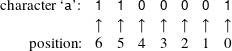
A memory location is accessed via an address:
The byte of data representing the character ‘‘Q’’ is at address 0012 while we have a ‘‘D’’ at address 0017. If you have a lot of memory, you need to use very large numbers as addresses.
Next up to consider is the central processing unit, the CPU, within a classical computer. It’s a cliché, but it really is like the brain of the computer. It controls executing a sequence of instructions that can do arithmetic, move data in and out of memory, use designated extra-fast memory called registers within the processor, and conditionally jump somewhere else in the sequence. The latest processors can help in memory management for interpreted programming languages and can even generate random numbers.
Physically, CPUs are today made from transistors, capacitors, diodes, resistors, and the pathways that connect them all into an integrated circuit. We differentiate between these electronic circuits and the logic circuits that are implemented using them.
In 1965, Gordon Moore extrapolated from several years of classical processor development and hypothesized that we would be able to double the speed of and number of transistors on a chip roughly every two years. [6] When this started to lose steam, engineers worked out how to put multiple processing units within a computer. These are called cores.
Within a processor, there can be special units that perform particular functions. A floating-point unit (FPU) handles fast mathematical routines with numbers that contain decimals. An arithmetic logic unit (ALU) provides accelerated hardware support for integer arithmetic. A CPU is not limited to having only one FPU or ALU. More may be included within the architecture to optimize the chip for applications like High Performance Computing (HPC).
Caches within a CPU improve performance by storing data and instructions that might be used soon. For example, instead of retrieving only a byte of information from storage, it’s often better to pull in several hundred or thousand bytes near it into fast memory. This is based on the assumption that if the processor is now using some data it will soon use other data nearby. Very sophisticated schemes have been developed to keep the cores busy with all the data and instructions they need with minimal waiting time.
You may have heard about 32- or 64-bit computers and chosen an operating system based on one or the other. These numbers represent the word size of the processor. This is the ‘‘natural’’ size of the piece of data that the computer usually handles. It determines how large an integer the processor can handle for arithmetic or how big an address it can use to access memory.
In the first case, for a 32-bit word we use only the first 31 bits to hold the number and the last to hold the sign. Though there are variations on how the number is stored, a common scheme says that if that sign bit is 1 the number is negative, and zero or positive if the bit is 0.
For addressing memory, suppose as above that the first byte in memory has address 0. Given a 32-bit address size, the largest address is 232−1. This is a total of 4,294,967,296 addresses, which says that 4 gigabytes is the largest amount of memory with which the processor can work. With 64 bits you can ‘‘talk to’’ much more data.
Question 2.1.1
What is the largest memory address a 64-bit processor can access?
In advanced processors today, data in memory is not really retrieved or placed via a simple integer address pointing to a physical location. Rather, a memory management unit (MMU) translates the address you give it to a memory location somewhere within your computer via a scheme that maps to your particular hardware. This is called virtual memory.
In addition to the CPU, a computer may have a separate graphics processing unit (GPU) for high-speed calculations involving video, particularly games and applications like augmented and virtual reality. The GPU may be part of the motherboard or on a separate plug-in card with 2, 4, or more gigabytes of dedicated memory. These separate cards can use a lot of power and generate much heat but they can produce extraordinary graphics.
Because a GPU has a limited number of highly optimized functions compared to the more general purpose CPU, it can be much faster, sometimes hundreds of times quicker at certain operations. Those kinds of operations and the data they involve are not limited to graphics. Linear algebra and geometric-like procedures make GPUs good candidates for some AI algorithms. [11] Even cryptocurrency miners use GPUs to try to find wealth through computation.
A quantum computer today does not have its own storage, memory, FPU, ALU, GPU, or CPU. It is most similar to a GPU in that it has its own set of operations through which it may be able to execute some special algorithms significantly faster. How much faster? I don’t mean twice as fast, I mean thousands of times faster.
A GPU is a variation on the classical architecture while a quantum computer is something entirely different.
You cannot take a piece of classical software or a classical algorithm and directly run it on a quantum system. Rather, quantum computers work together with classical ones to create new hybrid systems. The trick is understanding how to meld them together to do things that have been intractable to date.
2.2 The power of two
For a system based on 0s and 1s, the number 2 shows up a lot in classical computing. This is not surprising because we use binary arithmetic, which is a set of operations on base 2 numbers.
Most people use base 10 for their numbers. These are also called decimal numbers. We construct such numbers from the symbols 0, 1, 2, 3, 4, 5, 6, 7, 8, and 9, which we often call digits. Note that the largest digit, 9, is one less than 10, the base.
A number such as 247 is really shorthand for the longer 2 × 10² + 4 × 101 + 7 ×100. For 1,003 we expand to 1 × 10³ + 0 × 102 + 0 × 101 + 3×100. In these expansions we write a sum of digits between 0 and 9 multiplied by powers of 10 in decreasing order with no intermediate powers omitted.
We do something similar for binary. A binary number is written as a sum of bits (0 or 1) multiplied by powers of 2 in decreasing order with no intermediate powers omitted. Here are some examples:
| 0 | = 0 × 20 |
| 1 | = 1 × 20 |
| 10 | = 1 × 21 + 0 × 20 |
| 1101 | = 1 × 23 + 1 × 22 + 0 × 21 + 1 × 20 |
The ‘‘10’’ is the binary number 10 and not the decimal number 10. Confirm for yourself from the above that the binary number 10 is another representation for the decimal number 2. If the context doesn’t make it clear whether binary or decimal is being used, I use subscripts like 102 and 210 where the first is base 2 and the second is base 10.
If I allow myself two bits, the only numbers I can write are 00, 01, 10, and 11. 112 is 310 which is 22 − 1. If you allow me 8 bits then the numbers go from 00000000 to 11111111. The latter is 28 − 1.
For 64 bits the largest number I can write is a string of sixty four 1s which is
We do binary addition by adding bits and carrying.
| 0 + 0 | = 0 |
| 1 + 0 | = 1 |
| 0 + 1 | = 1 |
| 1 + 1 | = 0 carry 1 |
Thus while 1 + 0 = 1, 1 + 1 = 10. Because of the carry we had to add another bit to the left. If we were doing this on hardware and the processor did not have the space to allow us to use that extra bit, we would be in an overflow situation. Hardware and software that do math need to check for such a condition.
2.3 True or false?
From arithmetic let’s turn to basic logic. Here there are only two values: true and false. We want to know what kinds of things we can do with one or two of these values.
The most interesting thing you can do to a single logical value is to replace it with the other. Thus, the not operation turns true into false, and false into true:
not true = false
not false = true
For two inputs, which I call p and q, there are three primary operations and, or, and xor. Consider the statement ‘‘We will get ice cream only if you and your sister clean your rooms.’’ The result is the truth or falsity of the statement ‘‘we will get ice cream.’’
If neither you nor your sister clean your rooms, or if only one of you clean your room, then the result is false. If both of you are tidy, the result is true, and you can start thinking about ice cream flavors and whether you want a cup or a cone.
Let’s represent by (you, sister) the different combinations of you and your sister, respectively, having done what was asked. You will not get ice cream for (false, false), (true, false), or (false, true). The only combination that is acceptable is (true, true). We express this as
true and true = true
true and false = false
false and true = false
false and false = false
More succinctly, we can put this all in a table
| p = you | q = your sister | p and q |
| true | true | true |
| true | false | false |
| false | true | false |
| false | false | false |
where the first column has the values to the left of the and, and the second column has the values to the right of it. The rows are the values and the results. This is called a ‘‘truth table.’’
Another situation is where we are satisfied if at least one of the inputs is true. Consider ‘‘We will go to the movie if you or your sister feed the dog.’’ The result is the truth or falsity of the statement ‘‘we will go to the movie.’’
| p | q | p or q |
| true | true | true |
| true | false | true |
| false | true | true |
| false | false | false |
Finally think about a situation where we care about one and only one of the inputs being true. This is similar to or except in the case (true, true) where the result is false. It is called an ‘‘exclusive or’’ and written xor. If I were to say, ‘‘I am now going to the restaurant or going to the library,’’ then one of these can be true but not both, assuming I mean my very next destination.
Question 2.3.1
How would you state the inputs and result statement for this xor example?
| p | q | p xor q |
| true | true | false |
| true | false | true |
| false | true | true |
| false | false | false |
There are also versions of these that start with n to mean we apply not to the result. This means we apply an operation like and, or, or xor and then flip true to false or false to true. This ‘‘do something and then negate it’’ is not common in spoken or written languages but they are quite useful in computer languages.
nand is defined this way:
true nand false = not (true and false) = true
It has this table of values:
| p | q | p nand q |
| true | true | false |
| true | false | true |
| false | true | true |
| false | false | true |
I leave it to you to work out what happens for nor and nxor. These n-versions seem baroque and excessive now but several are used in the next section.
Question 2.3.2
Fill in the following tables based on the examples and discussion above.
| p | q | p nor q |
| true | true | |
| true | false | |
| false | true | |
| false | false |
| p | q | p nxor q |
| true | true | |
| true | false | |
| false | true | |
| false | false |
Instead of true and false we could have used 1 and 0, respectively, which hints at some connection between logic and arithmetic.
2.4 Logic circuits
Now that we have a sense of how the logic works, we can look at logic circuits. The most basic logic circuits look like binary relationships but more advanced ones implement operations for addition, multiplication, and many other mathematical operations. They also manipulate basic data. Logic circuits implement algorithms and ultimately the apps on your computer or device.
We begin with examples of the core operations, also called gates.
To me, the standard gate shapes used in the United States look like variations on spaceship designs.
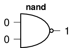
Rather than use true and false, we use 1 and 0 as the values of the bits coming into and out of gates.


This gate has two inputs and one output. It is not reversible because it produces the same output with different inputs. Given the 0 output, we cannot know which example produced it. Here are the other gates we use, with example inputs:

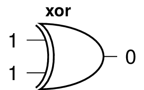
The symbol ‘‘⊕’’ is frequently used for the xor operation.
The not gate has one input and one output. It is reversible: if you apply it twice you get back what you started with.

People who study electrical engineering see these gates and the logic circuits you can build from them early in their training. This is not a book about electrical engineering. Instead, I want you to think of the above as literal building blocks. We plug them together, pull them apart, and make new logic circuits. That is, we’ll have fun with them while getting comfortable with the notion of creating logic circuits that do what we want.
I connect the output of one not gate to the input of another to show you get the same value you put in. x can be 0 or 1.

If we didn’t already have a special nand gate we could build it.
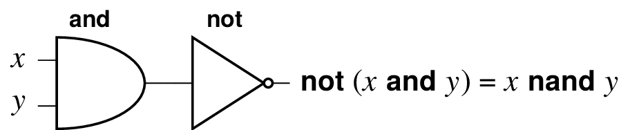
Note how we can compose gates to get other gates. We can build and from nand and not.
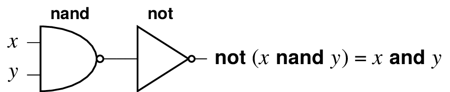
From this you can see that we could shrink the collection of gates we use if we desired. From this last example, it’s technically redundant to have and, nand, and not, but it is convenient to have them all. Let’s keep going to see what else we can construct.
Even though a gate like nand has two inputs, we can push the same value into each input. We show it this way:

What do we get when we start with 0 or 1 and run it through this logic circuit? 0 nand 0 = 1 and 1 nand 1 = 0. This behaves exactly like not! This means if we really wanted to, we could get rid of not. With this, having only nand we could drop not and and. It’s starting to seem that nand has some essential building block property.
By stringing together four nand gates, we can create an xor gate. It takes three to make an or gate. It takes one more of each to make nxor and nor gates, respectively.
Every logical gate can be constructed from a logic circuit of only nand gates. The same is true for nor gates. nand and nor gates are called universal gates because they have this property. [7]
It would be tedious and very inefficient to have all the basic gates replaced by multiple nand gates, but you can do it. This is how we would build or:

For the binary logic gates that have two inputs and one output, there are only eight possibilities, the four possible inputs 0/0, 0/1, 1/0, and 1/1 together with the outputs 0 and 1. Like or above, you can string together combinations of nands to create any of these eight gates.
Question 2.4.1
Show how to create the nor gate only from nand gates.
We looked at these logic circuits to see how classical processing is done at a very low level. We return to circuits and the idea of universal gates again for quantum computing in section 9.2 .
So far this has really been a study of classical gates for their own sakes. The behavior, compositions, and universality are interesting, but don’t really do much fascinating yet. Let’s do some math!
2.5 Addition, logically
Using binary arithmetic as we discussed in section 2.2 ,
| 0 + 0 | = 0 |
| 1 + 0 | = 1 |
| 0 + 1 | = 1 |
| 1 + 1 | = 0 carry 1 |
Focusing on the value after the equal signs and temporarily forgetting the carrying in the last case, this is the same as what xor does with two inputs.


We did lose the carry bit but we limited ourself to having only one output bit. What gate operation would give us that 1 carry bit only if both inputs were also 1, and otherwise return 0? Correct, it’s and! So if we can combine the xor and the and and give ourselves two bits of output, we can do simple addition of two bits.
Question 2.5.1
Try drawing a circuit that would do this before peeking at what follows. You are allowed to clone the value of a bit and send it to two different gates.
Question 2.5.2
Did you peek?

where A, B, S, and C are bits. The circuit takes two single input bits, A and B, and produces a 2-bit answer CD.
| A + B | = CS |
| 0 + 0 | = 00 |
| 1 + 0 | = 01 |
| 0 + 1 | = 01 |
| 1 + 1 | = 10 |
A full-adder has an additional input that is called the carry-in. This is the carry bit from an addition that might precede it in the overall circuit. If there is no previous addition, the carry-in bit is set to 0.

The square contains a circuit to handle the inputs and produce the two outputs.
Question 2.5.3
What does the circuit look like?
By extending this to more bits with additional gates, we can create classical processors that implement full addition. Other arithmetic operations like subtraction, multiplication, and division are implemented and often grouped within the arithmetic logic unit (ALU) of a classical processing unit.
For addition, the ALU takes multibit integer inputs and produces a multibit integer output sum. Other information can also be available from the ALU, such if the final bit addition caused an overflow, a carry-out that had no place to go.
ALUs contain circuits including hundreds or thousands of gates. A modern processor in a laptop or smartphone uses integers with 64 bits. Given the above simple circuit, try to estimate how many gates you would need to implement full addition.
Modern-day programmers and software engineers rarely deal directly with classical circuits themselves. Several layers are built on top of them so that coders can do what they need to do quickly.
If I am writing an app for a smartphone that involves drawing a circle, I don’t need to know anything today about the low-level processes and circuits that do the arithmetic and cause the graphic to appear on the screen. I use a high-level routine that takes as input the location of the center of the circle, the radius, the color of the circle, and the fill color inside the circle.
At some point a person created that library implementing the high-level routine. Someone wrote the lower-level graphical operations. And someone wrote the very basic circuits that implement the primitive operations under the graphical ones.
Software is layered in increasing levels of abstraction. Programming languages like C, C++, Python, Java, and Swift hide the low-level details. Libraries for these languages provide reusable code that many people can use to piece together new apps.
There is always a bottom layer, though, and circuits live near there.
2.6 Algorithmically speaking
The word ‘‘algorithm’’ is often used generically to mean ‘‘something a computer does.’’ Algorithms are employed in the financial markets to try to calculate the exact right moment and price at which to sell a stock or bond. They are used in artificial intelligence to find patterns in data to understand natural language, construct responses in human conversation, find manufacturing anomalies, detect financial fraud, and even to create new spice mixtures for cooking.
Informally, an algorithm is a recipe. Like a recipe for food, an algorithm states what inputs you need (water, flour, butter, eggs, etc.), the expected outcome (for example, bread), the sequence of steps you take, the subprocesses you should use (stir, knead, bake, cool), and what to do when a choice presents itself (‘‘if the dough is too wet, add more flour’’).
We call each step an operation and give it a name as above: ‘‘stir,’’ ‘‘bake,’’ ‘‘cool,’’ and so on. Not only do we want to overall process to be successful and efficient, but we construct the best possible operations for each action in the algorithm.
The recipe is not the real baking of the bread, you are doing the cooking. In the same way, an algorithm abstractly states what you should do with a computer. It is up to the circuits and higher-level routines built on circuits to implement and execute what the algorithm describes. There can be more than one algorithm the produces the same result.
Operations in computer algorithms might, for example, add two numbers, compare whether one is larger than another, switch two numbers, or store or retrieve a value from memory
Quantum computers do not use classical logical gates, operations, or simple bits. While quantum circuits and algorithms look and behave very differently from their classical counterparts, there is still the idea that we have data that is manipulated over a series of steps to get what we hope is a useful answer.
2.7 Growth, exponential and otherwise
Many people who use the phrase ‘‘exponential growth’’ use it incorrectly, somehow thinking it only means ‘‘very fast.’’ Exponential growth involves, well, exponents. Here’s a plot showing four kinds of growth: exponential, quadratic, linear, and logarithmic.

I’ve drawn them so they all intersect at a point but afterwards diverge. After the convergence, the logarithmic plot (dot dashed) grows slowly, the linear plot (dashed) continues as it did, the quadratic plot (dotted) continues upward as a parabola, and the exponential one shoots up rapidly.
Take a look at the change in the vertical axis, the one I’ve labeled resources with respect to the horizontal axis, labeled problem size. As the size of the problem increases, how fast does the amount of resources needed increase? Here a resource might be the time required for the algorithm, the amount of memory used during computation, or the megabytes of data storage necessary.
When we move a certain distance to the right horizontally for problem size, the logarithmic plot increases vertically at a rate proportional to the inverse of the size (1/problem size), the linear plot increases at a constant rate for resources that does not depend on problem size. The quadratic plot increases at a vertical rate that is proportional to problem size. The exponential plot increases at a rate that is proportional to its current resources.
The logarithm is only defined for positive numbers. The function log10(x) answers the question ‘‘to what power must I raise 10 to get x?’’. When x is 10, the answer is 1. For x equals one million, the answer is 6. Another common logarithm function is log2 which substitutes 2 for 10 in these examples. Logarithmic functions grow very slowly.
Examples of growth are
| resources | = 2 × log10(problem size) |
| resources | = 4 × (problem size) |
| resources | = 0.3 × (problem size)2 |
| resources | = 7.2 × 3 problem size |
This means that for large problem size, the exponential plot goes up rapidly and then more rapidly and so on. Things can quickly get out of hand when you have this kind of positive exponential growth.
If you start with 100 units of currency and get 6% interest compounded once a year, you will have 100 (1 + 0.06) after one year. After two you will have 100 (1 + 0.06)(1 + 0.06) = 100 (1.06)2. In general, after t years you will have 100 (1.06)t. This is exponential growth. Your money will double in approximately 12 years.
Quantum computers will not be used over the next several decades to fully replace classical computers. Rather, quantum computing may help make certain solutions doable in a short time instead of being intractable. The power of a quantum computer potentially grows exponentially with the number of quantum bits, or qubits, in it. Can this be used to control similar growth in problems we are trying to solve?
2.8 How hard can that be?
Once you decide to do something, how long does it take you? How much money or other resources does it involve? How do you compare the worst way of doing it with the best?
When you try to accomplish tasks on a computer, all these questions come to bear. The point about money may not be obvious, but when you are running an application you need to pay for the processing, storage, and memory you use. This is true whether you paid to get a more powerful laptop or have ongoing cloud costs.
To end this chapter we look at classical complexity. To start, we consider sorting and searching and some algorithms for doing them.
Whenever I hear ‘‘sorting and searching’’ I get a musical ear worm for Bobby Lewis’ 1960 classic rock song ‘‘Tossin’ and Turnin’.’’ Let me know if it is contagious.
2.8.1 Sorting
Sorting involves taking multiple items and putting them in some kind of order. Consider your book collection. You can rearrange them so that the books are on the shelves in ascending alphabetic order by title. Or you can move them around so that they are in descending order by the year of publication. If more than one book was published in the same year, order them alphabetically by the first author’s last name.
When we ordered by title, that title was the key we looked at to decide where to place the book among the others. When we considered it by year and then author, the year was the primary key and the author name was the secondary key.
Before we sort, we need to decide how we compare the items. In words, we might say ‘‘is the first number less than the second?’’ or ‘‘is the first title alphabetically before the second?’’. The response is either true or false.
Something that often snags new programmers is comparing things that look like numbers either numerically or lexicographically. In the first case we think of the complete item as a number while in the second we compare character by character. Consider 54 and 8. Numerically, the second is less than the first. Lexicographically, the first is less because the character 5 comes before 8.
Therefore when coding you need to convert them to the same format. If you were to convert -34,809 into a number, what would it be? In much of Europe the comma is used as the decimal point, while in the United States, the United Kingdom, and several other countries it is used to separate groups of three digits.
Now we look two ways of numerically sorting a list of numbers into ascending order. The first is called a ‘‘bubble sort’’ and it has several nice features, including simplicity. It is horribly inefficient, though, for large collections of objects that are not close to being in the right order.
We have two operations: compare, which takes two numbers and returns true if the first is less than the second, and false otherwise; and swap, which interchanges the two numbers in the list.
The idea of the bubble sort is to make repeated passes through the list, comparing adjacent numbers. If they are out of order, we swap them and continue through the list. We keep doing this until we make a full pass where no swaps were done. At that point the list is sorted. Pretty elegant and simple to describe!
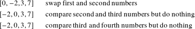
Let’s begin with a case where a list of four numbers is already sorted:
Now let’s look at
Now for the worst case with the list in reverse sorted order
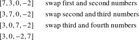
We did 3 comparisons and 3 swaps.
Second pass:

We did 3 comparisons and 2 swaps.
Third pass:
We did 3 comparisons and 1 swap.
Fourth pass:
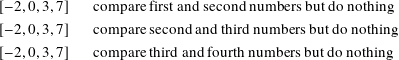
No swap, so we are done, and the usual 3 comparisons.
For this list of 4 numbers we did 12 comparisons and 6 swaps in 4 passes. Can we put some formulas behind these numbers for the worst case?
We had 4 numbers in completely the wrong order and so it took 4 full passes to sort them. For a list of length n we must do n − 1 comparisons, which is 3 in this example.
The number of swaps is the interesting number. On the first pass we did 3, on the second we did 2, the third we did 1, and the fourth we did none. So the number of swaps is
There is a formula that can help us with this last sum. If we want to add up 1, 2, and so on through a positive integer m, we compute ![]() .
.
Question 2.8.1
Try this out for m = 1, m = 2, and m = 3. Now see if the formula still holds if we add in m + 1. That is, can you rewrite
In our case, we have m = n − 1 and so we do a total of ![]() swaps. For n = 4 numbers in the list, this is none other than the 6 swaps we counted by hand.
swaps. For n = 4 numbers in the list, this is none other than the 6 swaps we counted by hand.
It may not seem so bad that we had to do 6 swaps for 4 numbers in the worst case, but what if we had 1,000 numbers in completely reversed order? Then the number of swaps would be
More formally, we say that the number of interesting operations used to solve a problem on n objects is O(f(n)) if there is a positive real number c and an integer m such that
To learn more
In the area of computer science called complexity theory, researchers try to determine the best possible f, c, and m to match the growth behavior as closely as possible. [1, Chapter 3] [9, Section 1.4]
If an algorithm is O(nt) for some positive fixed number t then the algorithm is of polynomial time. Easy examples are algorithms that run in O(n), O(n2), and O(n3) time.
If the exponent t is very large then we might have a very inefficient and impractical algorithm. Being of polynomial time really means that it is bounded above by something that is O(nt). We therefore also say that an O(log(n)) algorithm is of polynomial time since it runs faster that an O(n) algorithm.
Getting back to sorting, we are looking at the worst case for this algorithm. In the best case we do no swaps. Therefore when looking at a process we should examine the best case, the worst case, as well as the average case. For the bubble sort, the best case is O(n) while the average and worst cases are both O(n2).
If you are coding up and testing an algorithm and it seems to take a very long time to run, you likely either have a bug in your software or you have stumbled onto something close to a worst case scenario.
Can we sort more efficiently than O(n2) time? How much better can we do?
By examination we could have optimized the bubble sort algorithm slightly. Look at the last entry in the list after each pass and think about how we could have reduced the number of comparisons. However, the execution time is dominated by the number of swaps, not the number of comparisons. Rather than tinkering with this kind of sort, let’s examine another algorithm that takes a very different approach.
There are many sorting algorithms and you might have fun searching the web to learn more about the main kinds of approaches. You’ll also find interesting visualizations about how the objects move around during the sort. Computer science students often examine the different versions when they learn about algorithms and data structures.
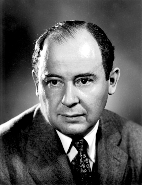
John von Neumann in the 1940s. Photo subject to use via the Los Alamos National Laboratory notice.
The second sort algorithm we look at is called a merge sort and it dates back to 1945. It was discovered by John von Neumann. [4]
To better see how the merge sort works, let’s use a larger data set with 8 objects and we use names instead of numbers. Here is the initial list:

We sort this in ascending alphabetic order. This list is now neither sorted nor in reverse order, so this is an average case.
We begin by breaking the list into 8 groups (because we have 8 names), each containing only one item.

Trivially, each group is sorted within itself because there is only one name in it. Next, working from left to right pairwise, we create groups of two names where we put the names in the correct order as we merge.
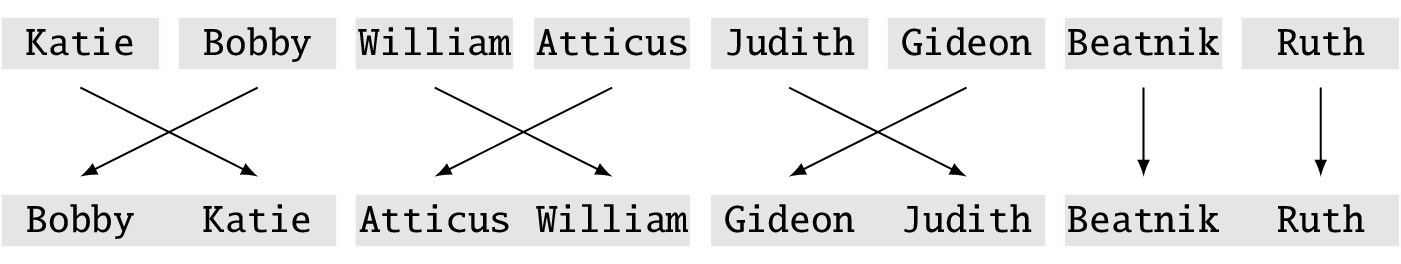
Now we combine the groups of two into groups of four, again working from left to right. We know the names are sorted within the group. Begin with the first name in the first pair. If it is less than the first name in the second pair, put it at the beginning of the group of four. If not, put the first name in the pair there.
Continue in this way. If a pair becomes empty, put all the names in the other pair at the end of the group of four, in order.

We finally create one group, merging in the names as we encounter them from left to right.

Among the variations of merge sort, this is called a bottom-up implementation because we completely break the data into chunks of size 1 and then combine.
For this algorithm we are not interested in swaps because we are forming new collections rather than manipulating an existing one. That is, we need to place a name in a new group no matter what. Instead the metric we care about is the number of comparisons. The analysis is non-trivial, and is available in algorithms books and on the web. The complexity of a merge sort is O(n log(n)). [1]
This is a big improvement over O(n2). Forgetting about the constant in the definition of ![]() and using logarithms to base 10, for n = 1000000 = 1 million, we have n2 = 1000000000000 = 1012 = 1 trillion, while log10(1000000) × 1000000 = 6000000 = 6 × 106 = 6 million. Would you rather do a million times more comparisons than there are names or 6 times the number of names?
and using logarithms to base 10, for n = 1000000 = 1 million, we have n2 = 1000000000000 = 1012 = 1 trillion, while log10(1000000) × 1000000 = 6000000 = 6 × 106 = 6 million. Would you rather do a million times more comparisons than there are names or 6 times the number of names?
In both bubble and merge sorts we end up with the same answer, but the algorithms used and their performance differ dramatically. Choice of algorithm is an important decision.
For the bubble sort we had to use only enough memory to hold the original list and then we moved around numbers within this list. For the merge sort in this implementation, we need the memory for the initial list of names and then we needed that much memory again when we moved to groups of 2. However, after that point we could reuse the memory for the initial list to hold the groups of 4 in the next pass.
By reusing memory repeatedly we can get away with using twice the initial memory to complete the sort. By being extra clever, which I leave to you and your research, this memory requirement can be further reduced.
Question 2.8.2
I just referred to storing the data in memory. What would you do if there were so many things to be sorted that the information could not all fit in memory? You would need to use persistent storage like a hard drive, but how?
Though I have focused on how many operations such as swaps and comparisons are needed for an algorithm, you can also look at how much memory is necessary and do a O( ) analysis of that. Memory-wise, bubble sort is O(1) and merge sort is O(n).
2.8.2 Searching
Here is our motivating problem: I have a collection S of n objects and I want to find out if a particular object target is in S. Here are some examples:
- Somewhere in my closet I think I have a navy blue sweater. Is it there and where? Here target = ‘‘my navy blue sweater.’’
- If I keep my socks sorted by the names of their predominant colors in my dresser drawer, are my blue argyle socks clean and available?
- I have a database of 650 volunteers for my charity. How many live in my town?
- I brought my kids to a magic show and I got volunteered to go up on stage. Where is the Queen of Hearts in the deck of cards the magician is holding?
With only a little thought, we can see that searching is at worst O(n) unless you are doing something strange and questionable. Look at the first object. Is it target? If so, look at the second and compare. Continue if necessary until we get to the nth object. Either it is target or target is not in S. This is a linear search because we go in a straight line from the beginning to the end of the collection.
If target is in S, in the best case we find it the first time and in the worst it is the nth time. On average it takes n/2 attempts.
To do better than this classically we have to know more information:
- Is S sorted?
- Can I access any object directly as in ‘‘give me the fourth object’’? This is called random access.
- Is S simply a linear collection of objects or does it have a more sophisticated data structure?
If S only has one entry, look at it. If target is there, we win.
If S is a sorted collection with random access, I can do a binary search.
Since the word ‘‘binary’’ is involved, this has something to do with the number 2.
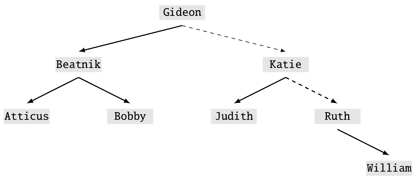
I now show this with our previously sorted list of names. The problem we pose is seeing if target = Ruth is in S. There are 8 names in the list. If we do a linear search it would take 7 tries to find Ruth.

Let’s take a different approach. Let m = n/2 = 4 which is near the midpoint of the list of 8 names.
In case m is not a whole number, we round up. Examine the mth = fourth name in S. That name is Gideon. Since S is sorted and Gideon < Ruth, Ruth cannot be in the first half of the list. With this simple calculation we have already eliminated half the names in S. Now we need only consider

There are 4 names and so we divide this in half to get 2. The second name is Katie. Since Katie ![]()
Ruth, Ruth is again not in the first half of this list. We repeat with the second half.

The list has length 2 and we divide this in half and look at the first name. Ruth! Where have you been?
We found Ruth with only 3 searches. If by any chance that last split and compare had not found Ruth, the remaining sublist would have had only one entry and that had to be Ruth since we assumed that name was in S. We located our target with only 3 = log2(8) steps.
Binary search is O(log(n)) in the worst case, but remember than we imposed the conditions that S was sorted and had random access. As with sorting, there are many searching techniques and data structures that can make finding objects quite efficient.
As an example of a data structure, look at the binary tree of our example names as shown in Figure 2.1. The dashed lines show our root to Ruth. To implement a binary tree in a computer requires a lot more attention to memory layout and bookkeeping.
Question 2.8.3
I want to add two more names to this binary tree, Richard and Kristin. How would you insert the names and rearrange the tree? What about if I delete Ruth or Gideon from the original tree?
Question 2.8.4
For extra credit, look up how hashing works. Think about the combined performance of searching and what you must do to keep the underlying data structure of objects in a useful form.
Entire books have been written on the related topics of sorting and searching. We return to this topic when we examine Grover’s quantum algorithm for locating an item in an unsorted list without random access in only O(√n) time in section 9.7.
If we replace an O(f(n)) algorithm with an O(√f(n)) one, we have made a quadratic improvement. If we replace it with a O(log(f(n))) algorithm, we have made an exponential improvement.
Suppose I have an algorithm that takes 1 million = 106 days to complete. That’s almost 2,740 years! Forgetting about the constant in the O() notation and using log10, a quadratic improvement would complete in 1,000 = 103 days, which is about 2.74 years. An exponential improvement would give us a completion time of just 6 days.
To learn more
There are many kinds of sorting and searching algorithms and, indeed, algorithms for hundreds of computational use cases. Deciding which algorithm to use in which situation is very important to performance, as we have just seen. For some applications, there are algorithms to choose the algorithm to use! [5] [9]
2.9 Summary
Classical computers have been around since the 1940s and are based on using bits, 0s and 1s, to store and manipulate information. This is naturally connected to logic as we can think of a 1 or 0 as true or false, respectively, and vice versa. From logical operators like and we created real circuits that can perform higher-level operations like addition. Circuits implement portions of algorithms.
Since all algorithms to accomplish a goal are not equal, we saw that having some idea of measuring the time and memory complexity of what we are doing is important. By understanding the classical case we’ll later be able to show where we can get a quantum improvement.
References
- [1]
-
Thomas H. Cormen et al. Introduction to Algorithms. 3rd ed. The MIT Press, 2009.
- [2]
-
R.W. Hamming. ‘‘Error Detecting and Error Correcting Codes’’. In: Bell System Technical Journal 29.2 (1950).
- [3]
-
R. Hill. A First Course in Coding Theory. Oxford Applied Linguistics. Clarendon Press, 1986.
- [4]
-
Institute for Advanced Study. John von Neumann: Life, Work, and Legacy. url: https://www.ias.edu/von-neumann.
- [5]
-
Donald E. Knuth. The Art of Computer Programming, Volume 3: Sorting and Searching. 2nd ed. Addison Wesley Longman Publishing Co., Inc., 1998.
- [6]
-
Gordon E. Moore. ‘‘Cramming more components onto integrated circuits’’. In: Electronics 38.8 (1965), p. 114.
- [7]
-
Ashok Muthukrishnan. Classical and Quantum Logic Gates: An Introduction to Quantum Computing. url: http://www2.optics.rochester.edu/users/stroud/presentations/muthukrishnan991/LogicGates.pdf.
- [8]
-
Oliver Pretzel. Error-correcting Codes and Finite Fields. Student Edition. Oxford University Press, Inc., 1996.
- [9]
-
Robert Sedgewick and Kevin Wayne. Algorithms. 4th ed. Addison-Wesley Professional, 2011.
- [10]
-
The Unicode Consortium. About the Unicode® Standard. url: http://www.unicode.org/standard/standard.html.
- [11]
-
B. Tuomanen. Explore high-performance parallel computing with CUDA. Packt Publishing, 2018.