4
Planes and Circles and Spheres, Oh My
No employment can be managed without arithmetic,
no mechanical invention without geometry.
Benjamin Franklin
In the last chapter we focused on the algebra of numbers and collections of objects that behave like numbers. Here we turn our attention to geometry and look at two and three dimensions. When we start working with qubits in chapter 7, we represent a single qubit as a sphere in three dimensions. Therefore, it’s necessary to get comfortable with the geometric side of the mathematics before we tackle the quantum computing aspect.
Topics covered in this chapter
4.2 The real plane
4.2.1 Moving to two dimensions
4.2.2 Distance and length
4.2.3 Geometric figures in the real plane
4.2.4 Exponentials and logarithms
4.3 Trigonometry
4.3.1 The fundamental functions
4.3.2 The inverse functions
4.3.3 Additional identities
4.4 From Cartesian to polar coordinates
4.5 The complex ‘‘plane’’
4.6 Real three dimensions
4.7 Summary
4.1 Functions
A function is one of the concepts in math that sounds pretty abstract but is really straightforward once you get experience with it. Thought of in terms of numbers, a function takes a value and returns one and only one value.
For example, for any real number, we can square it. That process is a function. For any non-negative real number, if we take the positive square root of it then we get another function. If we were to say we got both the positive and negative square roots, we would not have a function.
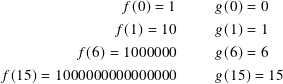
We use the notation f(x) for a function, meaning that we start with some value x, do something to it indicated by the definition of f, and the result is f(x). The f can be any letter or word, but we use f because the word ‘‘function’’ starts with it and we are not being especially creative. It’s common to see g and h but, really, we can use anything.
We write a function definition like f(x) = x2 or g(x) = √x or h(x) = 2x −3.
The set of values that we can use for x is called the domain of the function. The domain of f(x) = x2 could be the integers, the real numbers, the complex numbers, or any other set that makes sense. When considering real numbers, the domain of g(x) = √x is the set of non-negative real numbers, for example.
The range of a function is the set of values it produces. So if the domain of f(x) = x2 is R then the range is the set of all non-negative real numbers. The same is true for the absolute value |x|. I didn’t mention f(x) or g(x) or something similar when I said that |x| is a function.
It’s not mandatory to use the f(x) notation when the context makes it clear we have a function. We can also use the arrow notation x ↦ f(x) to show the input is x and the result is f(x).
When the range of function is some subset of R, we say that ‘‘f is real-valued.’’ Similarly we might say it is integer-valued or complex-valued.
Functions don’t have to work on or produce numeric inputs and outputs only. Consider the function c(n) on the integers that produces the color white if n is even and the color black if n is odd. Each integer is mapped to one of white or black, though an infinite number of integers are mapped to each color.
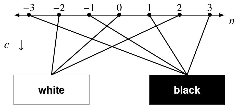
We can use another variation of the arrow notation to show the domain and range of a function.
A function that has only one value in its range is called constant. The function zero(x) = 0 is constant. So is the function sin2(x) + cos2(x), though you need to know the trigonometric identity to realize that.
I use x and n as the domain variables in the above examples. Just like f is only one possibility for the function name, we can use any letter or word for the domain variable. t is another common choice, especially when we think of the domain as real numbers representing time. Don’t use the same letter or word as the name of the function!
Question 4.1.1
What would be your personal function if we defined height(t) where t is your age in days?
Functions don’t have to be defined in a simple way with only one formula. They may be stated for portions of their domains. For example,
A real-valued function f on the real numbers is called linear if the following conditions hold:
- if x and y are real numbers then f(x + y) = f(x) + f(y), and
- if a is a real number then f(ax) = af(x).
This implies that f(ax + by) = af(x) + bf(y) for real numbers a, b, x, and y.
The only linear functions that map real numbers to real numbers look like f(x) = cx, for c a fixed value. We call such a c a constant. For example, f(x) = 7x or f(x) = −x. When we consider functions applied to collections that have more structure, the linear functions will be significantly less trivial.
What are the real-valued linear functions on the real numbers such that |f(x)| = |x| for any x? Since f(x) = cx, then
Can you reverse the effect of a function? If f(x) = 3x − 1 then if we apply g(x) = (1/3) x + 1/3 we get

g is the inverse of f because g(f(x)) = x. id(x) is its own inverse.
Question 4.1.2
Does f(x) = 5 have an inverse?
Question 4.1.3
What conditions do you need to impose on the domain of f(x) = x2 so that the positive √x is the inverse?
If f and g are functions such that g(f(x)) = x and f(g(y)) = y for all x and y in the domains of f and g, respectively, then f and g are invertible and one is the inverse of the other.
4.2 The real plane
When we were building up the structure of the integers, we showed the traditional number line

with the negative integers to the left of 0 and the positive ones to the right. Really, though, this was just part of the real number line

This is one-dimensional in that we need only one value, or coordinate, to locate a point uniquely on the line. For a real number x, we represent the point on the line by (x). For example, the point (−2.6) is between the markings −3 and −2. We use or omit the parentheses when it is clear from context whether we are referring to the point or the real number that gives its relative position from 0.

I drop the decimal points on the labels now that it is clear we have real numbers.
4.2.1 Moving to two dimensions
Now suppose the number line sits in two dimensions so that we extend upwards and downwards.

Since we need two coordinates for two dimensions, we position points with two real number x and y coordinates and label the point (x, y). These are called Cartesian coordinates after the mathematician René Descartes.
We positioned the point (1, 3) in the upper right side of the graph and (−5/2, −1) in the lower left. The horizontal line is called the x axis and the vertical line is the y axis. Cartesian coordinates are also called rectangular coordinates.

It may help you visualize this better if you think of the axes and points laid out on a table in front of you. This is the graph of the real plane, denoted R2.
One last bit of information to help us navigate: the axes divide the plane into four areas, or quadrants. The first quadrant, the one in the upper right, has both x and y positive.
Moving counterclockwise, the second quadrant has negative x and positive y. The third and fourth quadrants have x < 0 and y < 0, and x > 0 and y < 0, respectively.

Portrait of René Descartes (1596-1650) by Franz Hals. Painting is in the public domain.
4.2.2 Distance and length
Given two points in the real plane, how far apart are they?
What is the distance from (1, 1) to (4, 5)? This is equivalent to asking for the length of the line segment between the two points.
Are we talking about miles, kilometers, feet, centimeters, or what? Distance is usually mentioned in some particular unit. In math, we often don’t say which unless we are translating from a particular problem. We refer to ‘‘units’’ though we might note ‘‘x is measured in meters.’’ Unless necessary, we omit the particular kind of units.

The Pythagorean theorem states that in a right triangle, the square of the length of one side plus the square of the length of the other is equal to the square of the length of the hypotenuse.
We labeled the points on the corners of the triangle A, B, and C. One side of the triangle is the line segment AB, the other is BC, and the hypotenuse is AC.

If we use the notation |AB| to mean the length of the line segment AB, the theorem tells us
Let A = (1, 1), B = (4, 1), and C = (4, 5). By counting units on the axes we have |AB| = 3 and |BC| = 4. This means
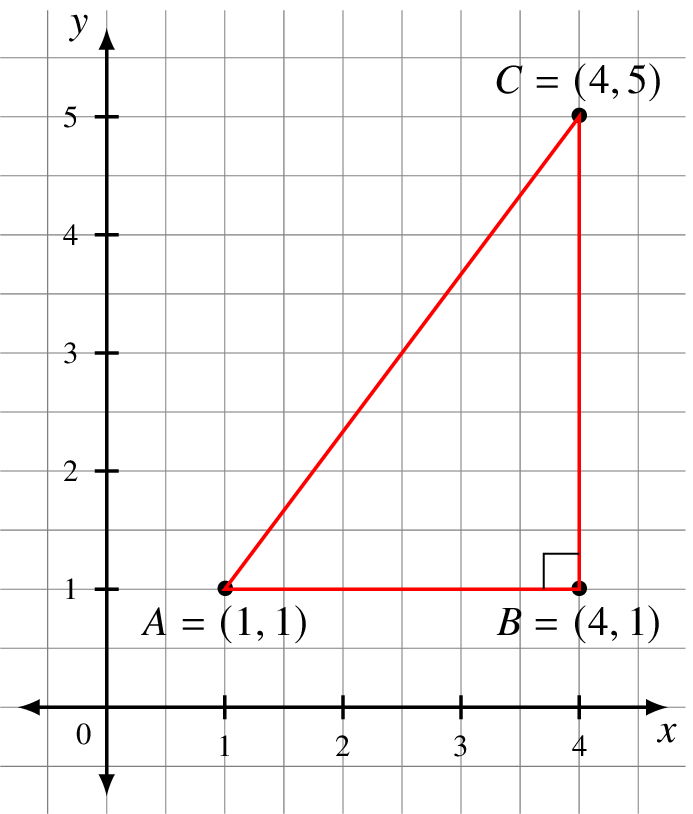
‘‘Counting units’’ along the x axis means to take the absolute value of the difference of the x coordinates. The similar statement holds for the y axis.
It’s rare for a triangle to have all its sides being natural numbers, but this is an example of a 3 : 4 : 5 triangle where things work out nicely. If you multiply or divide each side by the same natural number, the relationship still holds.
Question 4.2.1
A group of three natural numbers n : m : p is called a Pythagorean triple if n2 + m2 = p2. Find two more such triples that are not simple multiples of 3 : 4 : 5.
If the two sides each had length 1, the length of the hypotenuse would be √2.
Given two points in the real plane with coordinates (a, b) and (c, d), the distance between the two points is
4.2.3 Geometric figures in the real plane
Before we look at three dimensions and qubits, you must get comfortable with finding your way around R2 with the standard geometric figures like lines and circles. Let’s look at them and review general plotting of functions such as exponentials and logarithms.
Lines
Given two different points with coordinates (a, b) and (c, d), there is only one line you can draw between those points. The essential notion of a line is that when you move from one point to another, the ratio of the change in distance between the y coordinates and the change in distance between the x coordinates is constant. This ratio is called the slope of the line.
If (1, 1) is a point on the line and the slope is 2, for every unit we move in the x direction, we change twice that much in the y direction. Move 1 unit in x (that is, to the right), move 2 units in the y (up). Move -3 unit in x (that is, to the left), move −6 in the y (down).
For (x, y) to be on a line with slope m and given point (c, d), it must obey this equation
We begin by calculating the slope
This expresses y as a function of x. By the way, no one seems to know exactly why m is the standard variable name used for slope.

Plotting functions
When we have a real-valued function on all or part of R, we can plot it as we just saw for lines where y = f(x). If you were to do this by hand, you would choose enough values of x, compute f(x) for each, plot (x, f(x)) for each, and then connect the points. This may or may not be a good rendition of what it really looks like.
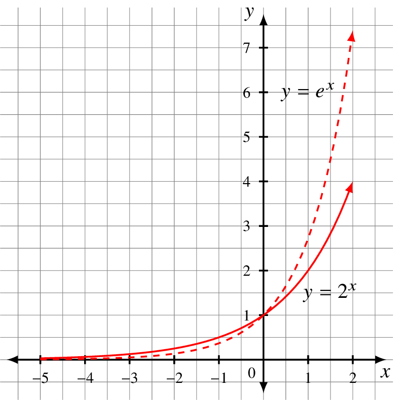
Let’s take ![]() . We let x have the integer values between -2 and 2.
. We let x have the integer values between -2 and 2.
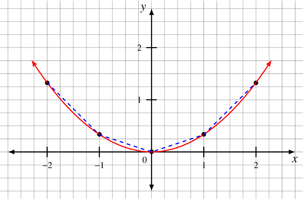
The outer smooth curve is the correct plot while the inner dashed one has straight lines connecting the few points we calculated.
It’s also possible to make mistakes while plotting because you inadvertently include a value that is not in the domain. Let ![]() when x ≠ 0. If we plot for x = −2, −1, 2, 1 and are careless we might see the dashed line plot below. The function is not defined at 0 and the plot looks more like the smooth solid curve.
when x ≠ 0. If we plot for x = −2, −1, 2, 1 and are careless we might see the dashed line plot below. The function is not defined at 0 and the plot looks more like the smooth solid curve.

We also say that ![]() is not continuous at x = 0.
is not continuous at x = 0.
Functions can be more sophisticated than mapping a number to a number. Let’s instead think of mapping a number to a point in the plane. If the input variable is t, we can think of the formula for the point as (g(t), h(t)). This includes the cases above because we can define g(t) to be t. This is called a parametrized function.
That is, rather than considering the function t2 from R to R and then plotting the points (t, t2), we instead directly plot the function t ↦ (t, t2) from R to R2. The plot of the function t ↦ (t2, t) looks like a parabola oriented horizontally.

Plotting parametrized functions can generate many beautiful graphs such as spirals and multi-petal flowers. Below is the plot of

Circles
A circle is defined by choosing one point as the center and then taking all points at a given fixed positive distance from that center. This distance is called the radius of the circle.
Let r be a positive real number that we use as the radius of the circle. If the coordinates of the center are ![]() and a point
and a point ![]() is distance r from the center, it satisfies the formula
is distance r from the center, it satisfies the formula
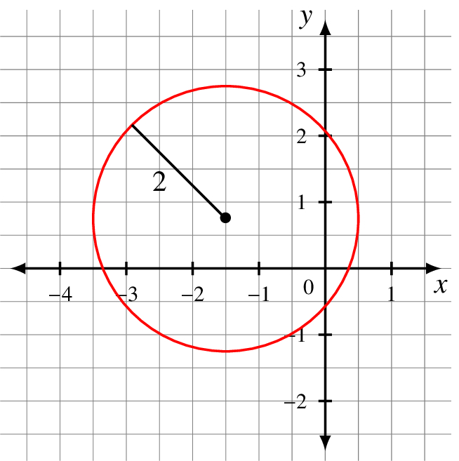
To the above right is the plot of the circle of radius 2 centered at (−1.5, 0.75). Its equation is (x + 1.5)2 + (y − 0.75)2 = r2.
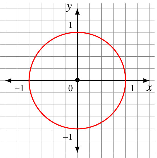
This is the plot of the unit circle of radius 1 centered at (0, 0), the origin: Its equation is x2 + y2 = 1.
Question 4.2.2
How would you write y as a function of x in the equation of the unit circle? What are the domain and range of the function?
4.2.4 Exponentials and logarithms
An exponential function has the form
When c is positive and 0 < a < 1, we have exponential decay.
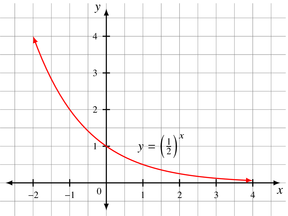
Radioactive decay follows this pattern.
If a > 1 we get exponential growth. Here are two examples of growth:
Moore’s Law, which was always more of an observation than a legally or physically binding statement, said that roughly every two years the computational power of a computer processor would double, its size would halve, and its energy requirements would also be cut in half. While this no longer seems to be the case, it was an example of exponential growth of power and decay of size and energy requirements. [5]
Compare the growth the exponential f(x) = 10x and linear g(x) = x functions.
Generally, exponential growth is something to be controlled or avoided in computation unless it somehow involves your money.
If exponential functions can show fast growth, logarithmic ones do the opposite. A logarithm is an inverse function of an exponential one.
The function log2(x) returns the answer to the question ‘‘to what power should I raise 2 to get x?’’ It is only defined for positive real numbers x.

If you work with computers long enough, you learn your powers of 2. log2 is called the binary logarithm.

The ‘‘inverse’’ behavior in the above means that x = 2log2(x) and x = log2(2x).
The natural logarithm is the inverse function to exponentiation by e. As a function name and shorthand for ‘‘loge’’, some authors use ‘‘ln’’ and others use ‘‘log’’. I use the latter.
For any positive base a, real number t, and positive real numbers x and y,
| loga(xy) | = loga(x) + loga(y) |
| loga(x/y) | = loga(x) − loga(y) |
| loga(xt) | = t loga(x) |
Question 4.2.3
Work out the details of deriving this formula. Show your work.
4.3 Trigonometry
Trigonometry is the study of triangles, angles, and length. The Greek word trig¯onon means ‘‘triangle’’ and metron means ‘‘measure.’’ For the most part we restrict ourselves to triangles with hypotenuse equal to 1, and so within the unit circle.
4.3.1 The fundamental functions
Many people have heard that a circle has 360 degrees, also written 360°. Why 360? If you look around the web you’ll find stories about ancient Mesopotamians, Egyptians, and base 60 number systems. Whatever the reason, 360 is a great number because it is divisible by so many other numbers like 2, 3, 4, 5, 6, 8, 10, 12, 15, and so on. That is, it’s easy to work with portions of 360° that are nice round whole numbers.
Degrees don’t really have a natural meaning in mathematics though. They are simply a convenient unit of measurement. Instead, we use radians.
A circle of radius r has circumference 2π r. If we go half way around the circle we cover a distance of π r. One quarter of the way cover ![]() .
.
When r = 1 we use fractions of 2π to determine how far around the circle we have gone. This is the radian measure of the corresponding angle. Half way around is π radians. If we go around three times we have 6π radians. This has real geometric meaning compared to degrees. When we move counterclockwise the radian measure is positive and it is negative when we move clockwise.
With either degrees or radians, we begin measuring the angle from the positive x axis.
Because we are dealing with a circle, an angle of 3π/4 radians lands us on the same point as does one of −5π/4 radians.

It’s customary to use Greek letters as variable names when we work with radians or degrees. The two most commonly used are θ (theta) and ϕ (phi).
Using θ as the measurement of the angle, consider the plot where P is a point on the unit circle with θ = π/3.
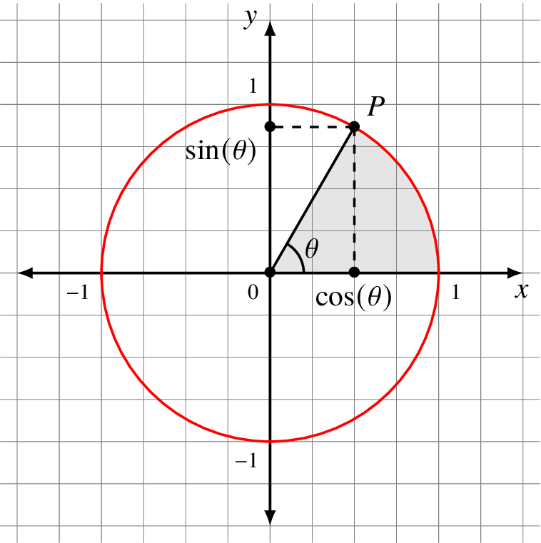
We define the function cos(θ), the cosine of θ, to be the x coordinate of the point P. Similarly, the function sin(θ), sine of θ is the y coordinate of P. Though we drew P in the first quadrant, we extend the definition to all points on the unit circle in all quadrants and on the axes.
The cosine is just an x coordinate and the sine is just a y coordinate. As functions they have many elegant properties, but it all comes down to the geometry of a radius 1 circle around the origin.
Because P is on the unit circle, it’s distance from the origin (0, 0) is 1. This means
Instead of writing the longer (cos(θ))2 in the above, I used the common shorthand cos2(θ).
If θ is negative, we consider |θ| but rotated clockwise from the positive x axis. Look at the above plot to convince yourself that ![]() and
and ![]() . While this is by no means a rigorous mathematical proof, developing your geometric intuition is more important here.
. While this is by no means a rigorous mathematical proof, developing your geometric intuition is more important here.
A function f like cos that has the property f(x) = f(−x) is called an even function. If f(−x) = −f(x) then the function is odd. sin is an odd function.
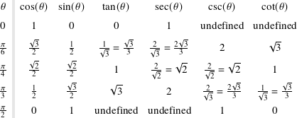
Another essential trigonometric function is the tangent, written tan(θ) and defined by
The tangent is the slope of the line segment from the origin (0, 0) to P.
The three remaining standard trigonometric functions are the secant, cosecant, and cotangent. These are defined, respectively, by
These are connected to the fundamental identity by dividing by cos2(θ) or sin2(θ).

These identities hold when the denominators are not 0.
4.3.2 The inverse functions
Do the trigonometric functions have inverses? Yes, but we need to be very careful at stating the domains and ranges. We also have to decide what to call them. Three notations are common for the inverse tangent:
The third version is common in programming languages like Python, Swift, C++, and Java. We use the middle one as it is traditional and relates to the arc that spans the angle in which we are interested.
The sine function gives its name to the archetypal example of a wave, a sinusoidal wave.

In the portion of the graph I’ve shown here, the plot crosses the x axis five times. On this graph sin(x) = 0 when x = −2π, −π, 0, π, and 2π. So what is arcsin(0)? We need to choose a range that ensures arcsin is single-valued and therefore a function.
arcsin(x) is a function with domain −1 ≤ x ≤ 1 and range π/2 ≤ arcsin(x) ≤ π/2.

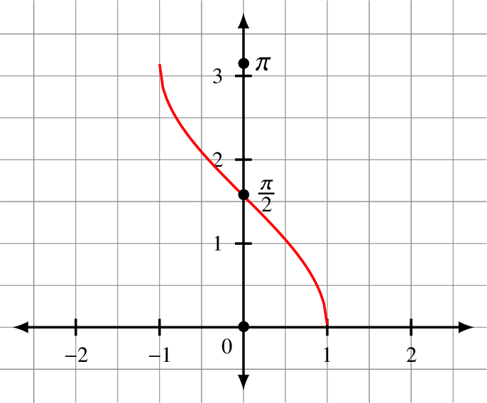
The inverse cosine arccos has a different range.
arccos(x) is a function with domain −1 ≤ x ≤ 1 and range 0 ≤ arccos(x) ≤ π.
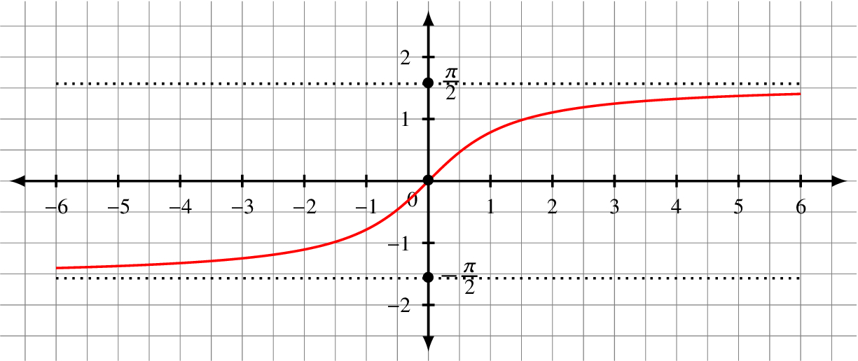
The inverse tangent arctan requires closer consideration because in the definition
arctan(x) is a function with domain all of R and range π/2 < arctan(x) < π/2.
4.3.3 Additional identities
There are several other trigonometric formulas which are useful. The sum and difference formulas express sin and cos when you have addition and subtraction of angles in the arguments.
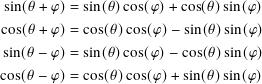
The last two follow from the first two because cos is an even function and sin is an odd function.
If we let θ = ϕ in the sum formulas, we get the double angle formulas.
4.4 From Cartesian to polar coordinates
Each point on the unit circle is uniquely determined by an angle ϕ given in radians such that 0 ≤ ϕ < 2π.
Even though a point on the unit circle is in R2, which is two-dimensional, it takes only one value, ϕ, to determine it. We lost the need for a second value by insisting that the point has distance 1 from the origin.
More generally, let P = (a, b) be a non-zero point (that is, a point which is not the origin) in R2. Let r = √a2 + b2 be the distance from P to the origin. Then the point
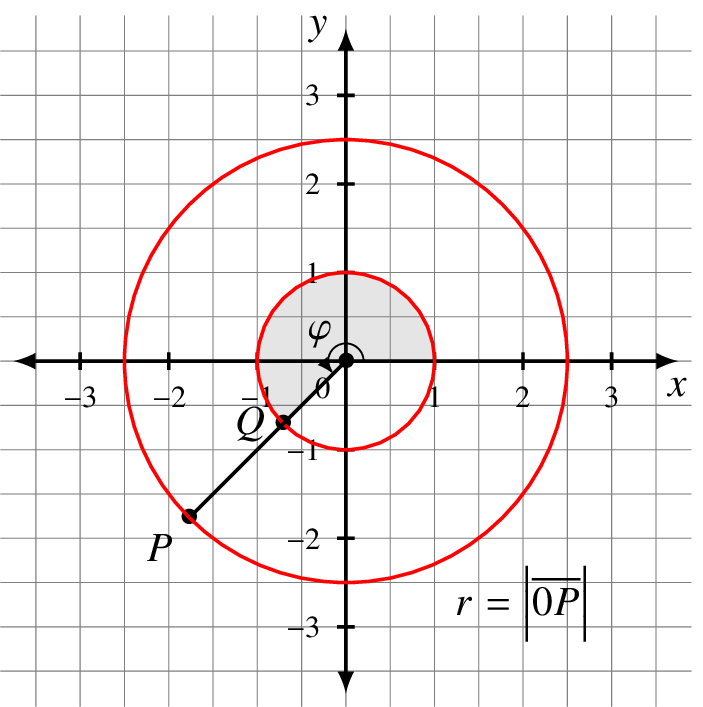
(r, ϕ) are called the polar coordinates of P. You may sometimes see the Greek letter ρ (rho) used instead of r.
Each non-zero point in R2 is uniquely determined by an angle ϕ given in radians such that 0 ≤ ϕ< 2π, and a positive real number r.
To uniquely identify P in this plot, r = 2.5 and ϕ = 5π/4.
4.5 The complex ‘‘plane’’
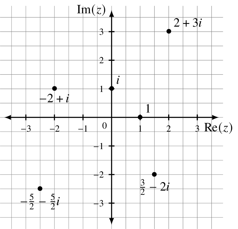
In the last chapter we discussed the algebraic properties of C, the complex numbers. We return to them again here to look at their geometry. For any point (a, b) in the real plane, consider the corresponding complex number a + bi.
In the graph of the complex numbers, the horizontal axis is the real part of the complex variable z and the vertical axis is the imaginary part. These replace the x and y axes, respectively.
The plot to the right shows several complex values. Despite appearances and some authors’ use of the terminology, that is not a complex plane. A plane has two dimensions. We visualized C, which is one-dimensional, in the two-dimensional real plane. We return to these issues about dimensions with respect to a field in the next chapter when we look at vector spaces.
Conjugation
Conjugation reflects a complex number across the horizontal Re(z) axis. If the number has 0 imaginary part, it is already on the Re(z) axis and so nothing happens.
If we conjugate a complex number z and then conjugate the result, we end up at z, the same place at which we started. Conjugation is its own inverse.

Question 4.5.1
What does conjugation do to 0? i?
Polar coordinates
As we saw above for the Cartesian plane R2, we can use polar coordinates for a point and so also for any non-zero complex number.
Each non-zero point z = a + bi in C is uniquely determined by an angle ϕ given in radians such that 0 ≤ ϕ < 2π, and a positive real number r = |z|. The arg function associates ϕ with z: ϕ = arg(z).
| z | = rcos(ϕ) + rsin(ϕ) i |
| = |z| cos(arg(z)) + |z| sin(arg(z)) i |
The angle ϕ is called the phase of z and |z| is its magnitude.
The term ‘‘phase’’ for the angle ϕ of a complex number is used in physics more than it is in mathematics. I introduce it here because we need it when we describe the representation of a qubit.

Any ϕ which is a non-zero integer multiple of 2π plus ϕ lands us on the same point, but we normalize our choice to be between 0 and 2π.
Instead of using the (r, ϕ) notation or the longer rcos(ϕ) + rsin(ϕ)i expression using polar coordinates, we adopt an exponential form incorporating both r and ϕ via Euler’s formula.
Euler’s formula
Leonhard Euler was a prolific eighteenth century mathematician who made many contributions in multiple fields of science. He was the first to prove the connection between the extension of the exponential function to the complex numbers and the a + bi notation involving polar coordinates. That is, he showed
To learn more
The proof of this is beyond the scope of this book. It falls with the branch of mathematics called complex analysis, which you may think of as the extension of calculus from the real numbers to the complex ones. [1] [3]
If z1 and z2 are non-zero complex numbers then |z1 z2| = |z1| × |z2| and arg(z1 z2) = arg(z1) + arg(z2). Expressed in long form, if
| z1 | = r1 cos(ϕ1) + r1 sin(ϕ1)i |
| z2 | = r2 cos(ϕ2) + r2 sin(ϕ2)i |

Using Euler’s formula, if z1 = r1 eϕ1 i and z2 = r2 eϕ2 i then

This is considerably simpler to use when we are multiplying or dividing complex numbers, but much less so when we are adding or subtracting. It also means that multiplying a complex number by eϕ i translates geometrically to rotating the complex number ϕ radians around 0. If ϕ is positive, the rotation is counterclockwise; for negative values it is clockwise.
If z = reϕ i then z = re−ϕ i.
Whether you think of a complex number as a real and imaginary part or as a phase and a magnitude, it holds two independent pieces of data represented as real numbers. This is very powerful and is one of the reasons why complex numbers show up in some unexpected places in physics and engineering.
4.6 Real three dimensions
When plotting in three dimensions, we need either three Cartesian coordinates (x0, y0, z0) or a radius r and two angles ϕ and θ.
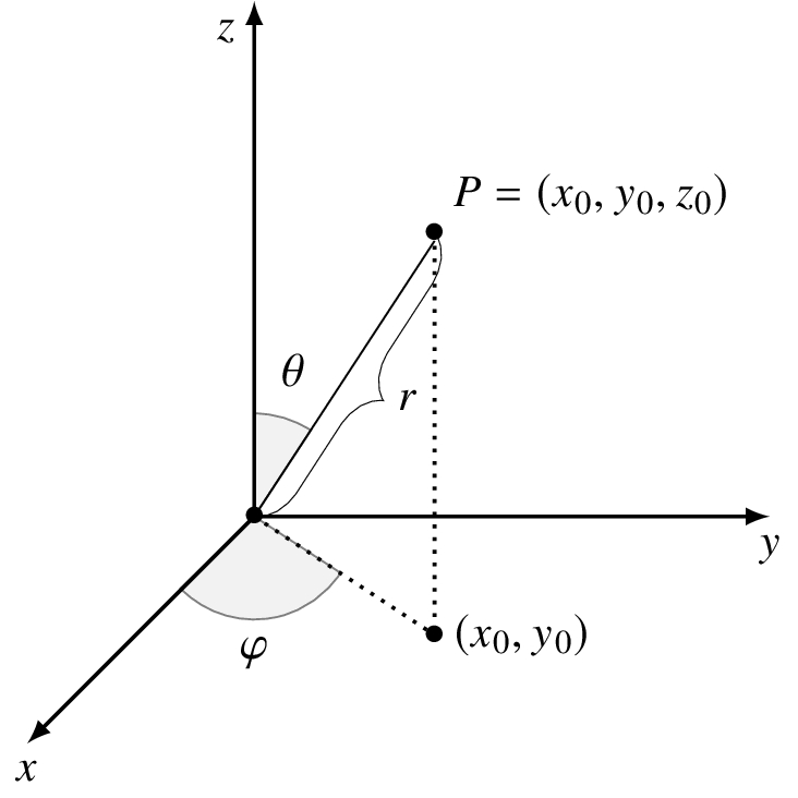
The radius r = |P| = √x02 + y02 + z02. ϕ is the angle from the positive x axis to the dotted line from (0, 0) to the projection (x0, y0) of P into the xy-plane. θ is the angle from the positive z axis to the line segment 0P.
That’s a lot to absorb, but it builds up systematically from what we saw in R2. When r = 1 we get the unit sphere in R3. It’s the set of all points (x0, y0, z0) in R3 where x02 + y02 + z02 = 1. The unit ball is the set of all points where x02 + y02 + z02 ≤ 1.
We return to this graphic frequently when we consider the Bloch sphere representation of a qubit.

If we were in four real dimensions we would need 4 coordinates (x, y, z, w). The unit hypersphere is the set of all points such that 1 = x2 + y2 + z2 + w2.
4.7 Summary
After handling algebra in the last chapter, we tackled geometry here. The concept of ‘‘function’’ is core to most of mathematics and its application areas like physics. Functions allow us to connect one or more inputs with some kind of useful output. Plotting functions is a good way to visualize their behavior.
Two- and three-dimensional spaces are familiar to us and we learned and reviewed the common tools to allow us to effectively use them. Trigonometry demonstrates beautiful connections between algebra and geometry and falls out naturally from relationships like the Pythagorean theorem.
The complex ‘‘plane’’ is like the real plane R2 but the algebra and geometry gives more structure than points alone can provide. Euler’s formula nicely ties together complex numbers and trigonometry in an easy-to-use notation that is the basis for how we define many quantum operations in chapter 7 and chapter 8 .
To learn more
Many readers were introduced to geometry in high school or its equivalent via theorems and proofs. If that part of the subject interests you, more advanced treatments explore axiomatic and geometric-algebraic approaches. [2] [4]
References
- [1]
-
L. V. Ahlfors. Complex Analysis. An introduction to the theory of analytic functions of one complex variable. 3rd ed. International Series in Pure and Applied Mathematics 7. McGraw-Hill Education, 1979.
- [2]
-
R. Artzy. Linear Geometry. Addison-Wesley series in mathematics. Addison-Wesley Publishing Company, 1974.
- [3]
-
J. B. Conway. Functions of One Complex Variable. 2nd ed. Graduate Texts in Mathematics 11. Springer-Verlag, 1978.
- [4]
-
H. S. M. Coxeter. Introduction to geometry. 2nd ed. Wiley classics library. John Wiley and Sons, 1999.
- [5]
-
Gordon E. Moore. ‘‘Cramming more components onto integrated circuits’’. In: Electronics 38.8 (1965), p. 114.