Chapter 11: Hash Object Memory Management

Anticipating performance and memory issues, the Bizarro Ball IT users have asked us to address several issues relating to performance, specifically data access times and memory management. If they should decide to proceed with the implementation of a follow-on project, they want to know what the options are as the amount of data grows. The generated data for our Proof of Concept included data for only one year. Any project will have to deal with multiple years of data.

This chapter focuses on the following three (overlapping) techniques:

1. Reducing the size of the key portion of the hash items.

2. Reducing the size of the data portion of the hash items.

3. Partitioning the data into groups that can be processed independently of one another.

This chapter addresses some of those concerns. Since the focus of this chapter is memory and performance and not the individual SAS programs, the IT and business users agreed that we need not annotate the programs to the same degree of detail as done for most of the previous programs.

Many of the examples here replicate samples in Chapters 6 and 10 by incorporating the techniques discussed here.

11.2 Memory vs. Disk Trade-Off

The data processing efficiency offered by the SAS hash object rests on two elements:

1. Its key-access operations, with the hashing algorithm running underneath, are executed in O(1) time.

2. Its data and underlying structure reside completely in memory.

These advantages over disk-based structures are easy to verify via a simple test. Consider, say, such ubiquitous data processing actions as key search and data retrieval against a hash table on the one hand, and against an indexed SAS data set on the other hand. For example, suppose that we have a SAS data set created from data set Dw.Pitches and indexed on a variable RID valued with its unique observation numbers. The DATA step creating it is shown as part of Program 11.1 below.

The DATA _NULL_ step in this program does the following:

1. Loads file Pitches into a hash table H with RID as its key and Pitcher_ID and Result as its data.

2. For all RID key-values in Pitches and an equal number of key-values not in Pitches, searches for RID in the table. If the key-value is found, retrieves the corresponding data values of Pitcher_ID and Result from the hash table into the PDV.

3. Does exactly the same against the indexed data set Pitches using its SAS index for search and retrieval.

4. Repeats both tests above the same number of times (specified in the macro variable test_reps below).

5. Calculates the summary run times for both approaches and reports them in the SAS log.

Program 11.1 Chapter 11 Hash Vs SAS Index Access Speed.sas

data Pitches (index=(RID) keep=RID Pitcher_ID Result) ;

set dw.Pitches ;

RID = _N_ ;

run ;

%let test_reps = 10 ;

data _null_ ;

dcl hash h (dataset: "Pitches", hashexp:20) ;

h.definekey ("RID") ;

h.defineData ("Pitcher_ID") ;

h.defineDone () ;

time = time() ;

do Rep = 1 to &test_reps ;

do RID = 1 to N * 2 ;

rc = h.find() ;

end ;

Hash_time = time() - time ;

time = time() ;

do Rep = 1 to &test_reps ;

do RID = 1 to N * 2 ;

set Pitches key=RID nobs=N ;

end ;

_error_ = 0 ; * prevent log error notes ;

Indx_time = time() - time ;

put "Hash_time =" Hash_time 6.2-R

/ "Indx_time =" Indx_time 6.2-R ;

stop ;

run ;

Note that the value of N used in both of these loops is initialized to the number of observations in Pitches because it is the variable specified in the SET statement NOBS= option. Also note that above, automatic variable _ERROR_ is set to zero to prevent the error notes in the log when the SET statement with the key=RID option fails to find the key.

When the program is run, the PUT statement prints the following in the SAS log:

Hash_time = 2.15

Indx_time = 21.58

As we see, a run with an equal number of search successes and failures shows that for the purposes of key search and data retrieval the SAS hash object works faster than the SAS index by about an order of magnitude. This is a consequence of both the difference between the search algorithms (the binary search versus hash search) and the access speed difference between memory and disk storage. The run-time figures above were obtained on the X64_7PRO platform. We told our IT users that if they are interested in trying it out under a different system, the program is included in the program file Chapter 11 Hash Vs SAS Index Access Speed.sas.

Note that the test above is strongly biased in favor of the SAS index because it always reads adjacent records which reduces paging, i.e., block I/O. Running it with the RID values picked randomly between 1 and N*2 shows that, in this case, the hash/(SAS index) speed ratio exceeds 50:1.

11.2.1 General Considerations

Holding data in memory comes at a price – the steeper, the larger the data volume handled in this manner is. At some point, it may approach or exceed the RAM capacity of the machine being used to process the data. As the IT users pointed out, the sample baseball data used in this book, though large and rich enough for our illustrative purposes, presents no challenge from this standpoint, as its largest data set of about 100 MB in size can nowadays be easily swallowed by the memory of even the most modest modern computing device. However, industrial practice, with its need to manipulate big and ever increasing volumes of data, presents a different picture. As the number of hash items, as well as the number of the hash variables and cardinality of the table keys grows, the hash memory footprint required to accomplish a task can easily reach into the territory of hundreds of gigabytes.

The sledge-hammer approach, of course, is to install more memory. Under some circumstances, it indeed makes sense. For instance, if it is vital for a large business to make crucial decisions based on frequently aggregated data (a "lead indicators" report in the managed health industry could be a good example), it appears to make more sense to invest in more RAM than to pay for coding around woeful hardware inadequacies. But as the authors have told the Bizarro Ball business users, our own experience of working on a number of industrial projects shows that this route can be blocked for a number of reasons.

Even if more machine resources can be obtained, it may turn out to be a temporary fix, working only till the time when the data volume grows or business demands change (for example, to require more hierarchical levels of data aggregation). In other words, crudely unoptimized code does not scale well. Thus, responsible SAS programmers do not merely throw a glaringly unoptimized program at the machine in hope that it will handle it and clamor for more hardware when it fails due to insufficient resources. Rather, they endeavor to avoid at least gross inefficiencies, regardless of whether or not the hardware has the capacity to cover for them at the moment, by taking at least obvious inexpensive measures to improve performance. Examples include making sure that the program reads and writes only the variables and records it needs, avoiding unnecessary sorts, etc.

Furthermore, sensible programmers aim to foresee how their code will behave if changes to the data, its volume, or business needs occur in the future – and structure their programs accordingly. Doing so requires more time and higher skill; yet, in the end, the result can prove to be well worth the price. Typical examples of this kind of effort are employing more efficient algorithms (e.g., the binary search rather than linear search) and making use of table lookup (e.g., via a format or a hash table) instead of sorting and merging, etc. This way, if (or rather when) the changes happen, chances are that the program will run successfully again in spite of them.

With the hash object, it is no different. Memory, though getting increasingly cheaper and abundant, is still a valuable resource. Hence, as the first line of defense, a programmer using the hash object should not overload it with unnecessary information for the sake of seemingly "simpler" coding and fewer lines of code. For instance, it is obvious that, to save memory, the hash table entry should contain only the variables and items it needs to do the job. Thus, using the argument tag ALL:"Y" with the DEFINEKEY and DEFINEDATA methods as a code shortcut (instead of defining only the needed variables in one way or another) must be judged accordingly. Likewise, if a hash table is used only for pure search (to find out if a key is there), using the MULTIDATA:"Y" argument tag is extraneous, as well as anything but a single short variable in the data portion.

As Bizarro Ball considers future expansion to more leagues, teams, and so on (e.g., some of the executives would like to offer the data analysis services to collegiate teams), expected data volumes may very well increase dramatically. Thus, hash memory management could be an important issue in the near term.

11.2.2 Hash Memory Overload Scenarios and Solutions

It is another question how to deal with more complex scenarios of the hash object running out of memory in spite of observing these obvious precautions. Typical circumstances under which it can occur include, but are not limited to, the following:

● A hash table is used as a lookup table for joining files. It can run out of memory if:

1. The file loaded into it has too many records.

2. The files are joined by a composite key with too many and/or too long components.

3. The satellite variables loaded into the data portion for future retrieval are too numerous and/or too long.

● A hash table is used as a container for data aggregation. It can run out of memory if:

1. The aggregation occurs at too many distinct key levels, consequently requiring too many unique-key table items.

2. The statistics to be aggregated are too numerous, and so are the corresponding data portion variables needed to hold them.

3. The keys are too numerous and/or long, and so are both the key and data portion variables needed to hold them (in the data portion, they are required in order to appear in the output).

Here are several tactics of resolving these hash memory overload problems which we will discuss in detail in the rest of this chapter:

● Take advantage of intrinsic pre-grouping. If the data input is sorted or grouped by one or more leading components of a composite key, use the BY statement to process each BY group separately, clearing the hash table after each group is processed. It works best if the BY groups are approximately equal in size.

● Reduce the key portion length. If the hash key is composite and the summary length of its components significantly exceeds 16 bytes, use the one-way hash function MD5 to shorten the entire key portion to a single $16 key. This can be done regardless of the total length of the composite key or the number of its components.

● Offload the data portion variables (use a hash index). It means that only the key (simple, composite, or its MD5 signature) is stored in the key portion, and only the file record identifier (RID) is stored in the data portion. When in the course of data processing a key-value is found in the table, the requisite satellite variables, instead of being carried in the data portion, are brought into the PDV by reading the input file via the SET POINT=RID statement. Effectively, this is tantamount to using a hash index created in the DATA step and existing for its duration.

● Use a known key distribution to split the input. If the values of some composite key component (or any if its bytes or group of bytes, for that matter) are known to correspond to a more or less equal number of distinct composite key-values, process the file using the WHERE clause separately for each such distinct value (or a number of distinct values) of such a component one at a time. As a result, the hash memory footprint will be reduced by the number of the separate passes.

● Use the MD5 function to split the input. Concatenate the components of the composite key and create an MD5 signature of the concatenated result. Because the MD5 function is a good hash function, the value of any byte (or a combination of bytes) of its signature will correspond to approximately the same number of different composite key-values. Then process the input in separate chunks based on these values using the WHERE clause as suggested above.

Note that these methods are not exclusive to themselves and can be combined. For example, you can both reduce the key portion length via the MD5 function and use the data portion offloading, any method can be combined with uniform input splitting, etc.

11.3 Making Use of Existing Key Order

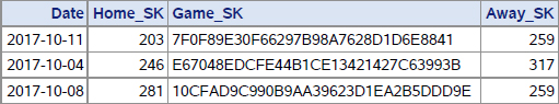
It often happens that the input we intend to process using a hash table is pre-sorted or pre-grouped by one or more leading variables of the composite key in question. For example, consider data set Dw.Runs where each run is recorded as a record. A subset of the file for two arbitrarily selected games is shown below. Note that the column From_obs is not a variable in the file; it just indicates the observations from which the records in the subset come.

Output 11.1 Chapter 11 Two Games from Dw.Runs

Suppose that we want to process it in some way using the hash object – for example, aggregate or unduplicate it – by the composite key (Game_SK,Top_Bot). In general, to do so, we would create a hash table keyed by the entire composite key and proceed as described earlier in the book according to the type of task at hand.

However, this file, though not sorted or grouped by the whole composite key, is intrinsically sorted by its leading component Game_SK, whose distinct values correspond to approximately an equal number of distinct key-values of the entire composite key. Since Game_SK is part of the composite key, no two composite key-values can be the same if their Game_SK values are different. It means that no composite key-value is shared between the groups of records with different values of Game_SK. Therefore, we can make use of Game_SK in the BY statement and process each BY group independently. After each BY

group is processed, we would add needed records to the output and clear the hash table to prepare it for processing the next BY group. From the standpoint of memory usage, doing so offers three advantages:

1. The hash table can now be keyed only by Top_Bot rather than by both Games_SK and Top_Bot. It shortens the key portion of the table.

2. Game_SK does not have to be replicated in the data portion. It shortens the data portion of the table.

3. The table has to hold the information pertaining to the largest BY group rather than the entire file. It reduces the maximum number of items the hash table must hold.

To see more clearly how this concept works, let us consider three very basic examples:

1. Data aggregation

2. Data unduplication

3. Joining data

11.3.1 Data Aggregation

Suppose that for each game (identified by Game_SK) we would like to find the score by each of the opposing teams. Since each record in the Runs file represents a run, it means that we would need to count the records for the top and bottom of the inning (i.e., the 2 values of Top_Bot) within each game. In other words, we would need to aggregate at each level of composite key (Game_SK,Top_Bot).

From the data aggregation chapter in this book (Chapter 8) we already know how a hash object frontal attack on this task can be carried out:

1. Use a hash table to count the records at each distinct (Game_SK,Top_Bot) key-value level.

2. Output its content when the input has been all processed.

Program 11.2 Chapter 11 Frontal Attack Aggregation.sas

data Scores (keep = Game_SK Top_Bot Score) ;

if _n_ = 1 then do ;

dcl hash h (ordered:"A") ;

h.defineKey ("Game_SK", "Top_Bot") ;

h.defineData ("Game_SK", "Top_Bot", "Score") ;

h.defineDone () ;

dcl hiter ih ("h") ;

end ;

do until (LR) ;

set Dw.Runs (keep = Game_SK Top_Bot) end = LR ;

if h.find() ne 0 then Score = 1 ;

else Score + 1 ;

h.replace() ;

end ;

do while (ih.next() = 0) ;

output ;

end ;

run ;

For detailed explanations of the mechanics of this basic aggregation process, see any of the examples in Chapter 8. Running the program, we get the following output for the two selected games shown in Output 11.1:

Output 11.2 Chapter 11 Dw.Runs Aggregates

Note that hash table H in its final state (before its content was written out to data set Scores) has 4 items, which corresponds to the number of output records.

However, we know that the input is pre-sorted by Game_SK. Thus, we can reduce both the key portion and data portion lengths by aggregating the same file one Game_SK BY group at a time. The changes from the frontal attack Program 11.2 are shown in bold:

Program 11.3 Chapter 11 Pregrouped Aggregation.sas

data Scores_grouped (keep = Game_SK Top_Bot Score) ;

if _n_ = 1 then do ;

dcl hash h (ordered:"A") ;

h.defineKey ("Top_Bot") ; ❶

h.defineData ("Top_Bot", "Score") ; ❷

h.defineDone () ;

dcl hiter ih ("h") ;

end ;

do until (last.Game_SK) ; ❸

set Dw.Runs (keep = Game_SK Top_Bot) ;

by Game_SK ;

if h.find() ne 0 then Score = 1 ;

else Score + 1 ;

h.replace() ;

end ;

do while (ih.next() = 0) ; ❹

output ;

end ;

h.clear() ; ❺

run ;

The program generates the same exact output as the frontal attack Program 11.2. For our two sample games, it is identical to Output 11.2 above. Let us go over some focal points of Program 11.3:

❶ When the key portion is defined, the leading component Game_SK of the composite key (Game_SK,Top_Bot) is omitted. Including it is unnecessary since the aggregation occurs by the level of Top_Bot alone within each separate BY value of Game_SK.

❷ The data portion does not contain Game_SK either. Its output value comes from the PDV as populated directly by the SET statement.

❸ The DoW loop, as opposed to iterating over the whole file, now iterates over one Game_SK BY group at a time per one execution of the DATA step (or one iteration of its implied loop). Note that the logical structure of the program remains intact. Also note that if the data were grouped, but not sorted by Game_SK, we could add the NOTSORTED option to the BY statement.

❹ At this point, hash table H contains the distinct key-values of Top_Bot and respective sums accumulated for the BY group just processed. Hash iterator IH linked to hash table H enumerates the table, and the data portion values of its items are written as records to the output data set Scores_grouped. Every BY group that follows adds its own records to the output file in the same manner.

❺ Now that the needed information (resulting from the processing of the current BY group) is written out, the table is cleared before the processing of the next BY group commences. Thus, the memory occupied by the hash data from the current BY group is released. Therefore, the largest hash memory footprint the program will create is that for the largest BY Game_SK group available in the file.

From the standpoint of saving hash memory, the more uniformly the values of Game_SK are distributed throughout the input file and the more distinct values of Game_SK (i.e., BY groups) we have, the better this method works. Running this program back-to-back with the frontal attack program with the FULLSTIMER system option turned on shows that, in this case, making use of the intrinsic leading key order cuts memory usage roughly by half. With a rather small file like Dw.Runs it may not matter much. However, in an industrial application working against billions of input records such a reduction can make a crucial difference.

Even if the distribution of the leading key(s) values is skewed, using the existing pre-grouping still saves hash memory by shortening both the key and data portions. In the examples shown above, the savings amount to 32 bytes per hash entry. Again, it may sound trivial but can be very significant if the items in a hash summary table should number in tens or hundreds of millions, as does indeed happen in reality. For example, if Bizarro Ball offered these services to college-level teams and they all accepted the offer, there would be orders of magnitude more games and thus Game_SK values.

It is all the more true that the composite key in question may have more than just two variables and may be pre-grouped by more than one. In general, a composite key (at whose level aggregation is requested) is composed of a number of leading key variables KL (by which the file is pre-grouped) and a number of trailing key variables KT:

(KL1, KL2, ..., KLn, KT1, KT2, ..., KTm)

In such a general case, both the key and data portions of the hash table would include:

("KT1", "KT2", ..., "KTm")

and the corresponding DoW loop similar to the loop shown in Program 11.3 would look as follows:

do until (last.KLn) ;

set ... ;

by KL1 KL2 ... KLn ;

...

end ;

The more leading keys KLn (by which the file is pre-grouped) are available relative to the number of the trailing keys KTm, the more hash memory this technique saves compared to the frontal attack by the whole composite key.

11.3.2 Data Unduplication

The same technique works, almost verbatim, for data unduplication. Suppose that we want to use the same file Dw.Runs to find, for each game, the inning and its half (i.e., top vs. bottom) in which each scoring player scored first. Let us look, for example, at the records for the first game in the file Dw.Runs (some variables are hidden, and the column From_obs indicates the respective observation numbers in the file):

Output 11.3 Chapter 11 Records for the First Game in Dw.Runs

From the data processing viewpoint, our task means that, for each game and runner, we need to output only the first record where the corresponding Runner_ID value is encountered. Thus, in the sample above, we would need to keep records 1, 2, 3, 5, 8, 11, and 13 and discard the rest. In other words, we would unduplicate the file based on the first distinct combination of key-values of composite key (Game_SK,Runner_ID).

If file Dw.Runs above were not pre-sorted by Game_SK, we would have to include the entire composite key (Game_SK,Runner_ID) in the key portion to execute a frontal attack as shown in Program 11.4 below. It uses the same logic as Program 10.2 in Chapter 10.

Program 11.4 Chapter 11 Frontal Attack Unduplication.sas

data First_scores ;

if _n_ = 1 then do ;

dcl hash h () ;

h.defineKey ("Game_SK", "Runner_ID") ;

h.defineData ("_N_") ;

h.defineDone () ;

dcl hiter ih ("h") ;

end ;

do until (LR) ;

set dw.Runs end = LR ;

if h.check() = 0 then continue ;

output ;

h.add() ;

end ;

run ;

The logic in the DO loop part requires no more than to check if the composite key-value from the current record of Dw.Runs is in table H. Therefore, the CHECK method is called to perform the Search operation. Hence, the data portion plays no functional role. However, as a hash table cannot exist without it, we are interested to make it as short as possible to minimize the hash memory footprint. The simplest way to do it is to define the data portion with a single numeric variable. Since in the context of the program it never interacts with the PDV, it does not matter which one we pick. The automatic variable _N_ chosen above to play the role of the dummy placeholder suits the purpose well since it is (a) numeric and (b) always present in the PDV. Therefore, no parameter type matching issues can arise.

For the input records of the game shown in Output 11.3, the program generates the following output:

Output 11.4 Chapter 11 Dw.Runs First Game Subset Unduplicated

However, if we make use of the fact that the file is intrinsically sorted by Game_SK, the program can be re-coded as shown in Program 11.5 below (the changes from Program 11.4 are shown in bold). This program generates exactly the same output as the frontal attack Program 11.4 above.

Program 11.5 Chapter 11 Pregrouped Unduplication.sas

data First_scores_grouped ;

if _n_ = 1 then do ;

dcl hash h () ;

h.defineKey ("Runner_ID") ; ❶

h.defineData ("_iorc_") ;

h.defineDone () ;

dcl hiter ih ("h") ;

end ;

do until (last.Game_SK) ; ❷

set dw.Runs (keep = Game_SK Inning Top_Bot Runner_ID) ;

by Game_SK ;

if h.check() = 0 then continue ;

output ;

h.add() ;

end ;

h.clear() ; ❹

run ;

❶ Note that Game_SK is no longer included in the key portion of table H.

❷ Instead of looping through the entire file, the DoW loop now iterates through each sorted group BY Game_SK one DATA step execution at a time.

❸ This is technically made possible by the BY statement, which sets last.Game_SK=1 each time the last game record is read and thus terminates the DoW loop.

❹ After the current game is processed, the hash table is cleared of all items, ceding the memory occupied by them to the operating system. Program control is then passed to the top of the DATA step, and the next game is processed.

Just like with data aggregation, taking advantage of partial pre-sorting saves hash memory in two ways:

● It reduces the key portion length by the summary length of the pre-sorted leading keys (in this case, just Game_SK).

● The ultimate number of items in the table corresponds to the game with the largest number of distinct runners. Contrast that with the frontal attack program above where the ultimate number of items is the number of distinct runners in the whole file. Note that from the perspective of understanding the data, we know that the number of runners in a given game can never exceed the total number of players on both teams. Thus, we have a virtual guarantee on the upper bound of the number of items in the hash table object at any given point in the data.

11.3.3 Joining Data

In the cases with data aggregation and unduplication, we have dealt with a single file partially pre-grouped by a leading component of the composite key. An inquisitive SAS programmer may ask whether one can take advantage, in a similar fashion, of partial pre-grouping if both files to be joined by using a hash table are identically pre-grouped by one leading key or more. The answer to this question is "Yes". However, the implementation is a tad more involved, as in this case it requires interleaving the files by the pre-grouped key components and a bit more of programming gymnastics.

To illustrate how this can be done, suppose that, for each runner record in data set Dw.Runs, we would like to obtain a number of related pieces of information from those records of data set Dw.AtBats where the value of variable Runs is not zero (indicating one or more runs). For example, we might want to know:

● The batter, i.e., what batter was responsible for the runner scoring.

● "How deep in the count" (reasonably standard baseball terminology for how many pitches there were in the at bat) the at bat went and what the ball/strike count was. The Dw.AtBats fields furnishing this information are Number_of_Pitches, Balls, and Strikes.

● Whether these were two out runs, i.e., scored when there had already been two outs. The Dw.AtBats field for this is Outs. (The batters and runners who contribute to runs with two outs are often considered to be clutch players.)

● Whether the runner scored as the result of a hit and the type of hit indicated by the values of variables Is_A_Hit and Result from file Dw.AtBats.

The files Dw.Runs and Dw.AtBats are linked by the following composite key:

(Game_SK, Inning, Top_Bot, AB_Number)

For the demo purposes, we have picked three games (the same from both files) and a few rows from each game. The samples are shown below in Output 11.5 and Output 11.6. Note that the column From_Obs is not a variable; it is included below just to show which observations have been picked. For Dw.Runs:

Output 11.5 Chapter 11 Dw.Runs Subset for Joining

For Dw.AtBats with Runs>0 and non-key variables limited to Batter_ID, Result, and Is_A_Hit:

Output 11.6 Chapter 11 Dw.AtBats Subset for Joining

To join the files by a hash object using a frontal attack, as in Program 6.6 Chapter 6 Left Join via Hash.sas, we have to:

● Key the hash table by all of the composite key variables.

● Place all of them, together with the satellite variables from Dw.AtBats, into the data portion.

Using this approach for the task at hand, we could proceed as follows.

Program 11.6 Chapter 11 Frontal Attack Join.sas

%let comp_keys = Game_SK Inning Top_Bot AB_Number ; ❶

%let data_vars = Batter_ID Is_A_Hit Result ;

%let data_list = %sysfunc (tranwrd (&data_vars, %str( ), %str(,))) ; ❷

data Join_Runs_AtBats (drop = _: Runs) ;

if _n_ = 1 then do ;

dcl hash h (multidata:"Y", ordered:"A") ;

do _k = 1 to countw ("&comp_keys") ; ❸

h.defineKey (scan ("&comp_keys", _k)) ;

end ;

do _k = 1 to countw ("&data_vars") ; ❹

h.defineData (scan ("&data_vars", _k)) ;

end ;

h.defineDone() ;

do until (LR) ;

set dw.AtBats (keep=&comp_keys &data_vars Runs

where=(Runs)) end = LR ;

h.add() ;

end ;

set dw.Runs ;

call missing (&data_list, _count) ;

do while (h.do_over() = 0) ;

_count = sum (_count, 1) ;

output ;

end ;

if not _count then output ;

run ;

❶ Assign the lists of key variables and satellite variables (from Dw.AtBats) to macro variables. Their resolved values are used later in the program instead of hard-coding the variable lists repeatedly.

❷ Create a comma-separated list of variable names in data_vars (using macro language facilities that we agreed to discuss with the IT users later) to be used in the CALL MISSING routine later.

❸ Place all the composite key variables in the key portion. Note that instead of passing their names to the DEFINEKEY method as a single comma-separated list of quoted names, the hash variables are added one at a time in a DO loop by passing a character expression with the SCAN function to the method call.

❹ Place the satellite variables into the data portion using the same looping technique.

In general, the program follows the principle of using a hash table to join files described in section 6.3.5 “Unique-Key Joins.” Running it results in the following joined output (for the sample rows from Output 11.5 and Output 11.6):

Output 11.7 Chapter 11 Dw.Runs and Dw.AtBats Subsets Join Result

From the standpoint of hash memory usage, this head-on approach has two disadvantages:

● All components of the composite key (Game_SK,Inning,Top_Bot,AB_Number) with the summary length of 40 bytes must be present in both the key and the data portions.

● The number of items in table H equals the total number of records in the file Dw.AtBats.

However, since files Dw.Runs and Dw.AtBats are both pre-sorted by their common leading key variables (Game_SK,Inning), both issues above can be addressed via processing each (Game_SK,Inning) BY group separately. But since now we have to deal with two files, it involves the extra technicality of interleaving them in the proper order and treating the records from each file differently within the same BY group. The differences between the head-on approach and this one are shown in bold:

Program 11.7 Chapter 11 Pregrouped Join.sas

%let comp_keys = Game_SK Inning Top_Bot AB_Number ;

%let data_vars = Batter_ID Is_A_Hit Result ;

%let data_list = Batter_ID,Is_A_Hit,Result ;

%let sort_keys = Game_SK Inning ; ❶

%let tail_keys = Top_Bot Ab_Number ; ❷

%let last_key = Inning ; ❸

data Join_Runs_AtBats_grouped (drop = _: Runs) ;

if _n_ = 1 then do ;

dcl hash h (multidata:"Y", ordered:"A") ;

do _k = 1 to countw ("&tail_keys") ;

h.defineKey (scan ("&tail_keys", _k)) ; ❹

end ;

do _k = 1 to countw ("&data_vars") ;

h.defineData (scan ("&data_vars", _k)) ;

end ;

h.defineDone() ;

end ;

do until (last.&last_key) ; ❺

set dw.atbats (in=A keep=&comp_keys &data_vars

Runs where=(Runs)) ❻

dw.runs (in=R keep=&comp_keys Runner_ID)

;

by &sort_keys ;

if A then h.add() ; ❼

if not R then continue ; ❽

call missing (&data_list, _count) ; ❾

do while (h.do_over() = 0) ;

_count = sum (_count, 1) ;

output ;

end ;

if not _count then output ;

end ;

h.clear() ;

run ;

❶ Assign the list of the leading key variable names by which the files are pre-sorted to macro variable sort_keys.

❷ Assign the list of the key variables names, except for those in sort_keys, to the macro variable tail_keys.

❸ Assign the name of the last key variable in sort_keys to the macro variable last_key. It is needed to properly specify the last.<variable-name> in the UNTIL condition of the DoW loop.

❹ Define the key portion only with the key variables in the tail_keys list – i.e., with those not in the sort_keys list. Note that, just as in the frontal attack program, they are defined dynamically one at a time.

❺ Use the DoW loop to process one (Game_SK,Inning) key-value BY group per DATA step execution. Note that the UNTIL condition includes the trailing key variable last.&last_key from the sort_keys list.

❻ Interleave Dw.AtBats and Dw.Runs – exactly in this sequence – using the key variables in the sort_keys list as BY variables. Doing so forces all the records from Dw.AtBats to come before those from Dw.Runs within each BY group. The automatic variables A and R assigned to the IN= data set option assume binary values (1,0) identifying the records from Dw.AtBats if A=1 (while R=0) and the records from Dw.Runs if R=1 (while A=0).

❼ Within each BY group, reading the records from Dw.AtBats before any records from Dw.Runs allows using the IF condition to load the hash table with the key and data values from Dw.AtBats only. If some BY group has no records from Dw.AtBats, so be it – all it means is that the hash table for this BY group will have no items.

❽ If this condition evaluates true, the record is not from Dw.Runs. Hence, we can just proceed to the next record.

❾ Otherwise, we use the standard Keynumerate operation to look up the current (Top_Bot,AB_Number) key-value pair coming from Dw.Runs in the hash table. If it is there, we retrieve the corresponding values of the satellite hash variables (listed in data_vars) into their PDV host variables. The loop outputs as many records as there are hash items with the current (Top_Bot,AB_Number) key-value in the current BY group. Calling the MISSING routine ensures that, if there is no match, the satellite variables from the data_vars list for the current output record have missing values regardless of the values that may have been retrieved in preceding records. (This is necessary to ensure proper output in the case of a left join.) The MISSING routine also initializes the value of _count for each new (Top_Bot,AB_Number) key-value.

Note that the "if not _count then output;" statement is needed only if a left join, rather than an inner join, is requested. With these two particular files, there is no difference, as every composite key in the comp_keys list in one file has its match in the other.

❿ After the current BY group is processed, the Clear operation is performed to empty out the table before it is loaded from the next BY group. Thus, in this program the topmost number of items in the hash table is controlled, not by the total number of records in file Dw.AtBats but by the number of records in its largest (Game_SK,Inning) BY group.

This program generates exactly the same output (Output 11.7) as the frontal attack Program 11.6.

Note that instead of hard-coding the lists data_list, tail_keys, and last_key, they can be composed automatically using the macro function %SYSFUNC:

%let comp_keys = Game_SK Inning Top_Bot AB_Number ;

%let data_vars = Batter_ID Is_A_Hit Result ;

%let sort_keys = Game_SK Inning ;

%let data_list = %sysfunc (tranwrd (&data_vars, %str( ), %str(,))) ; ❶

%let tail_keys = %sysfunc (tranwrd (&comp_keys, &sort_keys, %str())) ; ❷

%let last_key = %sysfunc (scan (&sort_keys, -1)) ; ❸

❶ Insert commas between the elements of the data_vars list by replacing the blanks between them with commas using the TRANWRD function.

❷ Take the sort keys out of the comp_keys list by replacing their names with single blanks using the TRANWRD function.

❸ Extract the trailing element from the sort_keys list using the SCAN function reading the list leftward (-1 means get the first element counting from the right instead of the left).

From now on, we are going to use this more robust functionality instead of hard-coded lists.

Although this program and the frontal attack Program 11.6 generate the same output, their hash memory usage is quite different. Tested under X64_7PRO, the frontal attack step consumes approximately 10 times more memory (about 12 megabytes) than the step-making use of the pre-sorted order. While a dozen of megabytes of RAM may be a pittance by today's standards, with much bigger data an order-of-magnitude reduction in hash memory footprint can make the difference between a program that successfully delivers its output on time and one that fails to run to completion.

11.4 MD5 Hash Key Reduction

In real-life industrial applications, data often needs to be processed by a number of long composite keys with numerous components of both numeric and character type. A typical example of such need is pre-aggregating data for online reporting at many levels of composite categorical variables. It is not uncommon in such cases to see a composite key grow to the length of hundreds of bytes. A large hash table keyed by such a multi-component key can easily present a serious challenge to the available memory resources.

It is all the more true that the entry size of a hash table in bytes does not merely equal the sum of the lengths of the variables in its key and data portions but usually exceeds it by a sizable margin. For example, let us consider a hash table below keyed by 20 numeric variables with only a single numeric variable in its data portion and use the ITEM_SIZE hash operator to find out what the resulting hash entry size will be. Then let us load the table with 1 million items and see if the DATA step memory footprint reported in the log is what we intuitively expect it to be.

Program 11.8 Chapter 11 Hash Entry Size Test.sas

data _null_ ;

array KN [20] (20 * 1) ;

dcl hash h() ;

do i = 1 to dim (KN) ;

h.defineKey (vname(KN[i])) ;

end ;

h.defineData ("KN1") ;

h.definedone() ;

Hash_Entry_Size = h.item_size ;

put Hash_Entry_Size= ;

do KN1 = 1 to 1E6 ;

h.add() ;

end ;

run ;

Running this step (on the X64_7PRO platform) results in the following printout in the SAS log:

Hash_Entry_Size=208

It would seem that, with 22 variables of 8 byte apiece, the hash entry size would be 176 bytes; yet in reality it is 208. Likewise, with 1 million items, we would expect the memory footprint of 167 megabytes or so, and yet the FULLSTIMER option reports that in actuality it is 208 megabytes, i.e., 25 percent larger. Though the hash entry size for given number, length, and data type of hash variables varies depending on the operating system (and whether it is 32-bit or 64-bit), the tendency of the hash memory footprint to be larger than perceived persists across the board.

Note that in order to determine the hash table entry size using the ITEM_SIZE attribute, it is unnecessary to load even a single item into the table. In fact, it makes good sense to do it against a (properly defined and created) empty table at the program planning stage if odds are that the table can be loaded with a lot of items. Estimating their future number and multiplying it by the hash entry size gives a fairly accurate idea of how much memory the table will consume when the program is actually run. In turn, the result may lead us to decide ahead of time whether any memory-saving techniques described here should be employed to reduce the hash memory footprint.

Table H used in the test above is actually rather small. The authors have encountered real-life projects where aggregate hash tables had to be keyed by composite keys with hash entry lengths upward of 400 bytes and would grow to hundreds of gigabytes of occupied memory if special measures to shorten their entries were not taken. One such measure, described above, makes use of an existing pre-sorted input order. However, in the situations where no such order exists, no variables can be relegated from the key portion of the hash table to the BY statement.

Thankfully, there exists another mechanism by means of which all key variables of the table (i.e., its composite key) can be effectively replaced by a single key variable of length $16 regardless of the number, data type, and lengths of the composite key components. "Effectively" means that from the standpoint of the data processing task result, using the replacement hash key is equivalent to using the composite key it replaces.

11.4.1 The General Concept

SAS software offers a number of one-way hash functions (note that, despite the name and using hashing algorithms, they are not related to the SAS hash object per se). The simplest and fastest of them is the MD5 function (apparently based on a well-known MD5 algorithm). It operates in the following manner:

signature = MD5 (<character_expression>) ;

If the defined length of character variable signature is greater than 16, MD5 populates it with 16 non-blank leading bytes followed by a number of trailing blanks. The non-blank part of the MD5 response (called the MD5 signature) is a 16-byte character string whose values are all different for all different values of any possible argument. This way, any character string has its own and only one MD5 signature value. (We will briefly address a theoretical possibility of deviation from this rule in section 11.10.1 “MD5 Collisions and SHA256.”)

The one-to-one relationship between the values of an MD5 argument and its response means that if we need to key a hash table by a composite key, we can instead:

● Concatenate its components into a character expression.

● Pass the expression to the MD5 function.

● Use its 16-byte signature in the key portion as a single simple key instead of the original composite key.

The advantage of this approach is a significant reduction of the key portion length and, consequently, of the entire hash entry length. Suppose, for instance, that the total length of the key portion composite key is 400 bytes, 25 times the length of its MD5 16-byte replacement key. Due to the internal hash object storage rules, it does not mean that the hash entry length will actually be reduced 25 times. For example, if the length of the keys is 400 bytes and the data portion has one 8-byte variable, replacing the composite key by its MD5 signature results in the total hash entry size of 64 bytes (as returned by the ITEM_SIZE operator on the X64_7PRO platform). While it is not the 25-fold reduction (which would be great, of course), the 7-fold hash memory footprint reduction is quite significant as well.

The concept delineated here is not unique to a particular data processing task. On the contrary, it applies to a great variety of them. As an alert IT user noticed, it is illustrated below using various data processing tasks. The intent is not to repeat what is already known but to drive home the point that the same concept works across the board and to demonstrate how it is implemented under different guises, at the same time offering the IT users a number of sample programs where specific technicalities of those guises have already been developed.

11.4.2 MD5 Key Reduction in Sample Data

Note that essentially the same technique has already been used in this book to generate sample data. To wit, in the program Chapter 5 GenerateSchedule.sas, the surrogate 16-byte character key Game_SK is created using the following expression:

Game_SK = md5 (catx (":", League, Away_SK, Home_SK, Date,Time)) ;

You can access the blog entry that describes this program from the author page at http://support.sas.com/authors. Select either “Paul Dorfman” or “Don Henderson.” Then look for the cover thumbnail of this book, and select “Blog Entries.” This variable is used as a universal surrogate key linking data files AtBats, Lineups, Pitches, and Runs to each other and to the data file Games. The latter cross-references each distinct value of Game_SK with the corresponding distinct value of composite key (League,Away_SK,Home_SK,Date,Time) along with other variables related to the specific game. Using this approach affords a number of advantages:

● Identifies each particular game in the data sets listed above using a single key instead of five separate keys.

● Reduces the record length of each of the data sets by (5*8-16)=22 bytes.

● Makes it easier and simpler to process (i.e., aggregate, unduplicate, join, etc.) these files anytime the program needs a game identifier, regardless of whether the hash object is used in the process or not.

● If the hash object is used, it needs a single $16 key Game_SK instead of the composite key with 5 components of 8 bytes each, thus reducing the hash table entry length. Also, it makes code shorter and clearer.

● This approach also provides great flexibility should the key structure need to change. For example, if the components of the key are augmented with additional variables, those fields can simply be included. For the example shown above that creates Game_SK, if an additional key (e.g., League Type: Majors, AAA, AA, A, Collegiate) is needed, the field League_Type would be included in the CATX function above and in our Games dimension table. No other program changes would be needed.

However, while having such a key as Game_SK already available as part of the data is of great utility, it does not mean that using the MD5 function to reduce the hash key portion length even further on the fly is not desirable or necessary. First, not all data collections have such a convenient provision as Game_SK in our sample data. Moreover, as we have seen in previous examples, data processing may involve more hash keys in addition to Game_SK. The examples in the rest of this section illustrate how this technique is used in terms of different data processing tasks.

In the following subsections we will illustrate the applicability of this approach to data aggregation, data unduplication and joining data just as we did in the section “Making Use of Existing Key Order”.

11.4.3 Data Aggregation

Suppose that we would like to expand the task of finding the score for each game already discussed above and find the score for each game and each inning using data set Dw.Runs. In other words, we need to count the records in the bottom and top of each inning of each game. To recap, for the two selected games shown in Output 11.1, the input data with the added variable Inning looks as follows:

Output 11.8 Chapter 11 Two Games from Dw.Runs

Using the hash object to solve the problem head-on is practically the same as in the first step of Program 11.3 Chapter 11 Pregrouped Aggregation.sas. The only difference is that now, in addition to Game_SK, we have to include both Top_Bot and Inning in the key portion and data portion:

Program 11.9 Chapter 11 Frontal Attack Aggregation Inning.sas

data Scores_game_inning (keep = Game_SK Inning Top_Bot Score) ;

if _n_ = 1 then do ;

dcl hash h (ordered:"A") ;

h.defineKey ("Game_SK", "Inning", "Top_Bot") ;

h.defineData ("Game_SK", "Inning", "Top_Bot", "Score") ;

h.defineDone () ;

dcl hiter ih ("h") ;

end ;

do until (LR) ;

set Dw.Runs (keep = Game_SK Inning Top_Bot) end = LR ;

if h.find() ne 0 then Score = 1 ;

else Score + 1 ;

h.replace() ;

end ;

do while (ih.next() = 0) ;

output ;

end ;

run ;

The output from the program (for our small visual input sample) looks as follows:

Output 11.9 Chapter 11 Frontal Attack Aggregation by (Game_SK,Top_Bot,Inning)

Note that all components of the composite key (Game_SK,Inning,Top_Bot) are included in the data portion of hash table H. Let us now use the MD5 function to replace the entire composite key with a single 16-byte key _MD5. The changes to the frontal attack Program 11.9 are shown below in bold:

Program 11.10 Chapter 11 MD5 Key Reduction Aggregation.sas

%let cat_length = 36 ; ❶

data Scores_game_inning_MD5 (keep = Game_SK Inning Top_Bot Score) ;

if _n_ = 1 then do ;

dcl hash h () ; ❷

h.defineKey ("_MD5") ;

h.defineData ("Game_SK", "Inning", "Top_Bot", "Score") ;

h.defineDone () ;

dcl hiter ih ("h") ;

end ;

do until (LR) ;

set Dw.Runs end = LR ;

length _concat $ &cat_length _MD5 $ 16 ; ❶

_concat = catx (":", Game_SK, Inning, Top_Bot) ; ❸

_MD5 = MD5 (_concat) ;

if h.find() ne 0 then Score = 1 ; ❹

else Score + 1 ;

h.replace() ;

end ;

do while (ih.next() = 0) ;

output ;

end ;

run ;

❶ Sizing _concat variable to accept the ensuing concatenation as $36 accounts for the actual system length of Game_SK ($16), Top_Bot ($1), 17 bytes for numeric variable Inning, plus 2 bytes for the CATX separator character. With only 3 key variables in question, it is not difficult to do; but with many more, this kind of hard-coding can become error-prone. So, instead of doing that, an astutely lazy programmer would notice that the key variables come from a SAS data set and use the system table Dictionary.Columns (or view Sashelp.Vcolumn) to populate the macro variable cat_length programmatically.

❷ No ORDERED argument tag is used here since the order by the _MD5 values is different from the order by the original composite key replaced by _MD5, and so ordering the output by _MD5 offers no benefit.

❸ Concatenate the components of the composite key using a colon as a separator. (Using the functions of the CAT family for the purpose is not without caveats. This is discussed in 11.10.1 MD5 Collisions and SHA256). Then feed variable _concat to the MD5 function. Its response _MD5 will be now used as the key-value.

❹ Invoke the standard data aggregation mechanism, except that now we are looking up, not the value of the original composite key, but its MD5 signature _MD5. As the relationship between them is one-to-one, it makes no difference for which one's distinct values Score is accumulated. Note that table H in this form is essentially a cross-reference between the _MD5 values in the key portion and the (Game_SK,Inning,Top_Bot) tuple in the data portion. Though the aggregation is done by the unique values of _MD5, the related values of the original composite key (Game_SK,Inning,Top_Bot) end up in the output.

For our two sample games, the program produces the following output:

Output 11.10 Chapter 11 MD5 Key Reduction Aggregation by (Game_SK,Top_Bot,Inning)

Note that its record order is different from that coming out of the frontal attack program. This is because the table is keyed by _MD5 whose values, though uniquely related to those of (Game_SK,Inning,Top_Bot), follow a totally different order. However, it does not present a problem because:

● Except for the inconvenience of eyeballing the unsorted result, the output is exactly the same.

● If we still want the file sorted by the original keys, it is not too much work since aggregate files are usually much smaller than unaggregated input. Also, the aggregated file can be indexed instead.

● If we wanted to display the values of the component variables used to create Game_SK, we could simply use it as a key to do a table lookup against the data set Games to get the desired values.

11.4.4 Data Unduplication

The same exact principle of using the MD5 function applies if we want to shorten the key portion when unduplicating data. Let us recall the DATA step of Program 11.4 Chapter 11 Frontal Attack Unduplication.sas in section 11.3.2. There, we used the composite hash key (Game_SK,Runner) to find and keep the records where each of its distinct key-values occurs first.

Using the MD5 function, we can now replace the composite key (Game_SK,Runner_ID) with a single 16-byte key _MD5 (the changes from Program 11.4 are shown in bold):

Program 11.11 Chapter 11 MD5 Key Reduction Unduplication.sas

%let cat_length = 34 ;

data First_scores_MD5 (drop = _:) ;

if _n_ = 1 then do ;

dcl hash h() ;

h.defineKey ("_MD5") ;

h.defineData ("_N_") ;

h.defineDone () ;

dcl hiter ih ("h") ;

end ;

do until (LR) ;

set dw.Runs end = LR ;

length _concat $ &cat_length _MD5 $ 16 ;

_concat = catx (":", Game_SK, Runner_ID) ;

_MD5 = MD5 (_concat) ;

if h.check() = 0 then continue ;

output ;

h.add() ;

end ;

run ;

The principal differences between the head-on and MD5 approaches are these:

● With the former, we store the distinct composite key-values (Game_SK,Runner) in the hash table and search the table to see if the key-value from the current record is already in the table.

● With the latter, we use the fact that the composite key-values of (Game_SK,Runner) and _MD5 are related as one-to-one and key the table with the latter.

Since in this case the sequence of the input records defines the output sequence, the relative record orders in both are the same (in other words, the unduplication process is stable), and the replacement of the composite key by _MD5 does not affect it. Note that if the SORT or SQL procedure were used to accomplish the task, the same record order would not (or would not be guaranteed to) be preserved.

For data unduplication the benefit of using the MD5 key-reduction technique is aided by the fact that nothing needs to be retrieved from the data portion (the very reason it is merely filled with the dummy placeholder _N_). So, the reduction of the hash entry length as a whole is roughly proportional to the reduction of the key portion length. In the example above, the shortening of the key length from 24 bytes to 16 may look trivial. However, under different circumstances it can reach an order of magnitude or more.

One such scenario is cleansing a data set where whole records, i.e., the values of all variables, have been duplicated for some reason, which is a typical occurrence in ETL processes. Imagine, say, that due to either programming or clerical error, some records in the data set Dw.Games have been completely duplicated. For example, suppose that the data for a given date were loaded twice. Since that did not occur when we created the sample data, we can emulate such a situation as follows:

Program 11.12 Chapter 11 Full Unduplication.sas (Part 1)

data Games_dup ;

set Dw.Games ;

do _n_ = 1 to floor (ranuni(1) * 4) ;

output ;

end ;

run ;

As a result, file Games_dup would have about twice as many records as the original, some records wholly duplicated. Output 11.8 below shows the first 8 records from Games_dup. The column From_obs is not a variable from the file but indicates the original observation numbers from Dw.Games.

Output 11.11 Chapter 11 Work.Games_dup Sample

Suppose that we need to cleanse the file by keeping only the first copy of each duplicate record while preserving the relative sequence of the input records. In other words, after the cleansing is done, our output should match the original file Dw.Games.

If we approached the task headlong using the frontal hash object attack, we would have to include all 9 variables from Games_dup (with the total byte length of 80) in the key portion, plus a dummy placeholder variable in the data portion. (Although, for this task, we do not need our key variables in the data portion since their output values come directly from the input file records, we still need at least one data portion variable due to the hash object design.) Having to include all input file variables in the key portion has its consequences:

● If the variables in the file are numerous, it will result in a large hash entry length.

● Even in this simple case with only 9 key portion variables (and 1 dummy data portion variable), the hash entry length on a 64-bit platform would be 128 bytes. For a real-world file with 100 million distinct records, it would result in the hash memory footprint close to 20 GB of RAM.

However, the problem can be easily addressed by using the MD5 key reduction approach because it replaces all key portion hash variables with a single 16-byte _MD5 key variable. This approach is demonstrated by the program below modified from Program 11.11 (the changes are shown in bold):

Program 11.12 Chapter 11 Full Unduplication.sas (Part 2)

%let cat_length = 53 ;

data Games_nodup (drop = _:) ;

if _n_ = 1 then do ;

dcl hash h() ;

h.defineKey ("_MD5") ;

h.defineData ("_N_") ;

h.defineDone () ;

dcl hiter ih ("h") ;

end ;

do until (LR) ;

set Games_dup end = LR ;

array NN[*] _numeric_ ; ❶

array CC[*] _character_ ;

length _concat $ &cat_length _MD5 $ 16 ;

_concat = catx (":", of NN[*], of CC[*]) ; ❷

_MD5 = MD5 (trim(_concat)) ;

if h.check() = 0 then continue ;

output ;

h.add() ;

end ;

run ;

Principally, the program is not much different from Program 11.11. The differences are noted below:

❶ The ARRAY statement in this form automatically incorporates all non-automatic numeric variables currently in the PDV into array NN. Likewise, the next statement automatically incorporates all non-automatic character variables currently in the PDV into array CC. Since during compile time at this point in the step the only non-automatic variables the compiler has seen are the variables from the descriptor of file Games_dup, these are the only variables the arrays incorporate. Note that it is incumbent upon the programmer to ensure that no other non-automatic variables get in the PDV before the arrays are declared; otherwise we may end up concatenating variables we do not need.

❷ Concatenate the needed variables into the MD5 argument using the shortcut array notation [*]. Note that since all the numeric variables are concatenated first followed by all the character variables (due to the order in which the arrays are declared), the concatenation order may differ from that of the variables in the file. This is okay since from the standpoint of the final result the concatenation order does not matter. This aspect of the technique (actually adding to its robustness) will be discussed in some more detail in the section "MD5 Argument Concatenation Ins and Outs".

For our first 8 sample records from Games_dup (Output 11.8), the program generates the following output:

Output 11.12 Chapter 11 Work.Games_dup Unduplicated

11.4.5 Joining Data

Let us now turn to the case of joining data already described and discussed earlier in the section “Joining Data”. There, Program 11.6 Chapter 11 Frontal Attack Join.sas represents a frontal attack where all components of the joining composite key (Game_SK, Inning,Top_Bot, AB_Number) are included in the key portion. In the program below, files Dw.Runs and Dw.AtBats are joined by a single key variable _MD5 instead. The differences between this code and the frontal attack Program 11.6 are shown in bold:

Program 11.13 Chapter 11 MD5 Key Reduction Join.sas

%let comp_keys = Game_SK Inning Top_Bot AB_Number ;

%let data_vars = Batter_ID Position_code Is_A_Hit Result ;

%let data_list = %sysfunc (tranwrd (&data_vars, %str( ), %str(,))) ;

%let keys_list = %sysfunc (tranwrd (&comp_keys, %str( ), %str(,))) ; ❶

%let cat_length = 52 ;

data Join_Runs_AtBats_MD5 (drop = _: Runs) ;

if _n_ = 1 then do ;

dcl hash h (multidata:"Y", ordered:"A") ;

h.defineKey ("_MD5") ; ❷

do _k = 1 to countw ("&data_vars") ;

h.defineData (scan ("&data_vars", _k)) ;

end ;

h.defineDone() ;

do until (LR) ;

set dw.AtBats (keep=&comp_keys &data_vars Runs

where=(Runs)) end = LR ;

link MD5 ; ❸

h.add() ;

end ;

set dw.Runs ;

link MD5 ; ❹

call missing (&data_list, _count) ;

do while (h.do_over() = 0) ;

_count = sum (_count, 1) ;

output ;

end ;

if not _count then output ;

return ;

MD5: length _concat $ &cat_length _MD5 $ 16 ; ❺

_concat = catx ("", &keys_list) ;

_MD5 = MD5 (_concat) ;

return ;

run ;

❶ A comma-separated list of key variable names is prepared to be used in the CATX function later.

❷ Rather than defining separate key variables in a loop, a single key variable _MD5 is defined.

❸ The LINK routine MD5 is called for every record from Dw.AtBats (the right side of the join) to concatenate the components of its composite key and pass the result to the MD5 function. Its signature _MD5 is added to table H along with the values of the data_vars list variables as a new hash item.

❹ For each record read from file Dw.Runs, the LINK routine MD5 is called again, now for the left side of the join. It generates the value of _MD5 key to be looked up in the hash table.

❺ The MD5 LINK routine is relegated to the bottom of the step to avoid repetitive coding. This way, we have only one set of code creating the _MD5 key for both data sets involved in the join; and this ensures that they are kept in synch (e.g., if the key structure should change for some reason, we would have only one set of code to change).

The principal difference between using the MD5 key reduction technique in this program and the programs used for data aggregation and unduplication is that since in this case we have two files (Dw.Runs and Dw.AtBats), the composite key needs to be converted to its MD5 signature for each record from both input files: For Dw.AtBats with the data to be loaded into the hash table and for Dw.Runs before the Keynumerate operation is invoked.

11.5 Data Portion Offload (Hash Index)

Thus far in this chapter, we have dealt with measures of reducing the length of the key portion by either moving its hash variables elsewhere or replacing them with a surrogate key. In the related examples, similar measures cannot be used to reduce the length of the data portion as well because its hash variables are needed for the Retrieve operation to extract the data into the PDV host variables.

However, in some cases the size of the data portion can be reduced by replacing the data retrieval from the hash table with extracting the same data directly from disk. Doing so effectively relegates the hash table to the role of a searchable hash index. This is a tradeoff: It sacrifices a small percentage of execution speed for the possibility to remove all data portion variables and replace them with a single numeric pointer variable. Two data processing tasks that benefit from this approach most readily are (a) joining data and (b) selective unduplication.

11.5.1 Joining Data

Let us return to our archetypal case of joining file Dw.Runs to file Dw.AtBats that we have already discussed in this chapter. See the section “Joining Data” for the task outline, visual data samples, and Program 11.6 Chapter 11 Frontal Attack Join.sas.

To recap, the task is to join the two files by composite key (Game_SK,Inning,Top_Bot,AB_Number) with the intent to enrich Dw.Runs with the satellite fields Batter_ID, Is_A_Hit, and Result from Dw.AtBats. In the frontal attack program, all these data fields are included in the data portion of the hash table. As mentioned earlier, we could potentially need to bring in many more fields depending on the questions asked about the game results. In real industrial applications, data portion variables may be much more numerous – the more of them, the greater hash memory footprint they impose. The question is, can their number be reduced; and if yes, then how?

To find out, let us observe that each observation in file Dw.AtBats can be marked by its serial number – that is, the observation number, in SAS terminology. This number is commonly referred to as the Record Identification Number (or RID Number or just RID). The idea here is to include RID in the data portion and load the table from Dw.AtBats with its RID values instead of the values of satellite variables. Then, for each hash item whose composite key (Game_SK,Inning,Top_Bot,AB_Number) matches its counterpart from Dw.Runs, the value of RID retrieved from the table can be used to extract the corresponding data directly from Dw.AtBats by using the SET statement with POINT=RID option. With these changes in mind, the frontal attack Program 11.6 can be re-coded this way (the changes are shown in bold):

Program 11.14 Chapter 11 Hash Index Join.sas

%let comp_keys = Game_SK Inning Top_Bot AB_Number ;

%let data_vars = Batter_ID Is_A_Hit Result ;

%let data_list = %sysfunc (tranwrd (&data_vars, %str( ), %str(,))) ;

data Join_Runs_AtBats_RID (drop = _: Runs) ;

if _n_ = 1 then do ;

dcl hash h (multidata:"Y", ordered:"A") ;

do _k = 1 to countw ("&comp_keys") ;

h.defineKey (scan ("&comp_keys", _k)) ;

end ;

h.defineData ("RID") ; ❶

h.defineDone() ;

do RID = 1 by 1 until (LR) ; ❷

set dw.AtBats (keep=&comp_keys Runs where=(Runs)) end = LR ;

h.add() ;

end ;

set dw.Runs ;

call missing (&data_list, _count) ;

do while (h.do_over() = 0) ; ❸

_count = sum (_count, 1) ;

set dw.Runs point = RID ; ❹

output ;

end ;

if not _count then output ;

run ;

❶ The data portion is defined with variable RID (i.e., Dw.AtBats observation number) and none of the satellite variables from the data_vars list.

❷ The sequential values of RID (i.e., the sequential observation number) are created here by incrementing RID up by 1 for each next record from Dw.Runs. Each value is inserted into the hash table as a new item along with the corresponding key-values from the comp_keys list. This way, the values of RID in the table are linked with the respective records from Dw.AtBats – and thus, with the respective values of the satellite variables.

❸ The Keynumerate operation searches the table for the key-values coming from each record from Dw.Runs and retrieves the RID values pointing to records in Dw.AtBats.

❹ If the PDV composite key-value accepted by the DO_OVER method is found in the table, the Keynumerate operation retrieves the RID values from the group of items with this key-value, one at a time, into PDV host variable RID. For each enumerated item, the retrieved value of RID is then used to access Dw.AtBats directly via the SET statement with the POINT=RID option, the value of RID pointing to the exact record we need. Thus, the values of the variables from the data_vars appear in the PDV because they are read directly from the file – not as a result of their retrieval from the hash table, as in the frontal attack program. (Note that since variable RID is named in the POINT= option, it is automatically dropped despite also being used as a DO loop index.)

Running this program generates exactly the same output as the frontal attack Program 11.6. The technique used in it is notable in a number of aspects:

● Memory-Disk Tradeoff. Offloading the data portion variables in this manner means that the satellite values are extracted from disk. Obviously, it is slower than retrieving them from hash table memory. However, this is offset by the fact that now those same variables need not be either loaded into or read from the hash table. More importantly, the action affecting performance most – namely, searching for a key – is still done using the hash lookup in memory.

● Performance. Testing shows that overall, the reduction in execution performance is insignificant because POINT= access (compared to SAS index access) is in itself extremely fast. If the satellites variables involved in the process are numerous and long, the trade-off is well worth the price, as it could reduce hash memory usage from the point where the table may fail to fit in memory (which would abend the program) to where the program still runs to completion successfully.

● Hash-Indexing. This technique has yet another interesting aspect. Effectively, by pairing RID in the hash table with its file record, we have created, for the duration of the DATA step, a hash index for file Dw.AtBats defined with the composite key from the comp_keys list. Both such hash index and a standard SAS index (residing in an index file) do essentially the same job: They search for RID given a key-value, simple or composite; and if it is found, both use the RID value to locate the corresponding record and extract the data from it. The difference is that the hash memory-resident index coupled with the hashing algorithm renders both the key search and data extraction (using the POINT=) option much faster.

● Hybrid Approach. The hash-indexing approach can be readily adapted to a hybrid situation where it may be expedient to have a few specific satellite variables defined in the data portion along with RID. This way, if programming logic dictates so, the values of these specific hash variables can be retrieved into their PDV host counterparts from the hash table without incurring extra I/O. And yet when it dictates, at some point, that the values from more (or, indeed, all) satellite variables are needed in the PDV, they can be extracted directly from disk via the SET statement with the POINT=RID option as shown above.

11.5.2 Selective Unduplication

The hash-indexing scheme as described above can work for any data task where a hash table is used to store satellite variables with the intent of eventually retrieving their hash values into the PDV – for example, for data manipulation or generating output. From this standpoint:

● Using it for simple file unduplication is pointless. Indeed, for this task the Retrieve operation is not used, and the only variable in the data portion is a dummy placeholder.

● By contrast, selective stable unduplication illustrated by Program 10.3 Chapter 10 Selective Unduplication via PROC SORT + DATA Step.sas can benefit from data portion disk offloading because, in this case, the variables in the data portion are retrieved from the hash table into the PDV in order to generate the output.

Let us recall the subset of file Dw.Games used to illustrate selective unduplication in Chapter 10. (Again, From_obs is not a data set variable. It just shows the observation numbers in Dw.Games related to the records in the subset below.)

Output 11.13 Chapter 11 Subset from Dw.Games for Selective Unduplication

To recap, the task lies in the following:

● Using this data, find the away team which each home team played last. In other words, we need to unduplicate the records for each key-value of Home_SK by selecting its record with the latest value of Date.

● Along with Home_SK, output the values of Away_SK, Date, and Game_SK from the corresponding record with the most recent value of Date.

● Note that this time, the requirements include the extra variable Game_SK in the output.

● Also note that in the data sample above, the records we want in the output are shown in bold.

To solve the task by using a frontal attack approach, it is enough to slightly modify Program 10.3 Chapter 10 Selective Unduplication via Hash:

Program 11.15. Chapter 11 Frontal Attack Selective Unduplication.sas

data _null_ ;

dcl hash h (ordered:"A") ; *Output in Home_SK order;

h.defineKey ("Home_SK") ;

h.defineData ("Home_SK", "Away_SK", "Date", "Game_SK") ;

h.defineDone () ;

do until (lr) ;

set dw.games (keep = Game_SK Date Home_SK Away_SK) end = lr ;

_Away_SK = Away_SK ;

_Date = Date ;

_Game_SK = Game_SK ;

if h.find() ne 0 then h.add() ;

else if _Date > Date then

h.replace (key:Home_SK, data:Home_SK, data:_Away_SK, data:_Date

, data:_Game_SK

) ;

end ;

h.output (dataset: "Last_games_hash") ;

stop ;

run ;

This program generates the following output for the records of our sample subset from Dw.Games:

Output 11.14 Chapter 11 Results of Frontal Attack Selective Unduplication

Note that the variables Away_SK and Game_SK are included in the data portion since their values are needed for the OUTPUT method call. Also, the temporary variables _Away_SK, and _Game_SK are included in the explicit REPLACE method call to update the data-values in table H for every input PDV value of Date greater than its presently stored hash value.

In this rather simple situation, there are only three satellite variables to be stored in the data portion and hard-coded in the explicit REPLACE method call. In other situations with many more satellite variables, two things with the frontal attack approach can become bothersome:

● With large data volumes and numerous satellite variables, hash memory can get overloaded.

● Hard-coding many arguments with the REPLACE method call is unwieldy and error-prone. In fact, even with a mere five arguments, as above, typing them in already gets pretty tedious.

However, both issues are easily addressed by using the hash index approach. In the program below, a hash table index keyed by Home_SK is used to keep the data portion variables that are not critical to the program logic out of the data portion. The program may seem to be a tad longer than the frontal attack. However, as we will see, its benefits far outweigh the cost of the few extra lines of code:

Program 11.16 Chapter 11 Hash Index Selective Unduplication.sas

data Last_away_hash_RID (drop = _:) ;

dcl hash h (ordered:"A") ;

h.defineKey ("Home_SK") ;

h.defineData ("Date", "RID") ; ❶

h.defineDone () ;

do _RID = 1 by 1 until (lr) ; ❷

set dw.Games (keep = Date Home_SK) end = lr ; ❸

_Date = Date ;

RID = _RID ; ❹

if h.find() ne 0 then h.add() ;

else if _Date > Date then

h.replace (key:Home_SK, data:_Date, data:_RID) ; ❺

end ;

dcl hiter hi ("h") ; ❻

do while (hi.next() = 0) ;

set dw.Games (keep = Home_SK Away_SK Game_SK) point = RID ; ❼

output ;

end ;

stop ;

run ;

❶ The data portion is defined with variables Date and RID. Note the absence of other variables needed in the frontal attack Program 11.15.

❷ A temporary variable _RID instead of RID is used to increment the record identifier to safeguard its values from being overwritten by the FIND method call.

❸ No need to keep Away_SK and Game_SK in this input, as their values on disk are linked to by RID.

❹ RID is repopulated with the memorized value of _RID to ensure its value is correct, just in case it may have been overwritten in the previous iteration of the DO loop by the FIND method call.

❺ RID in this explicit REPLACE call is used instead of Home_SK,_Away_SK, and _Game_SK. If we had more satellite variables, the _RID assigned to the argument tag DATA would replace the need to code any of them. Essentially, all references to the satellite variables here are replaced en masse with a single RID pointer to their location on disk.

❻ The hash iterator is used to render the output instead of the OUTPUT method since satellite variables needed in the output are no longer in the data portion (the same would be true of all other satellite variables if we had more of them). The satellite variable values will be extracted directly from the input file Dw.Games via POINT=RID option.

❼ Use RID as a record pointer to retrieve Home_SK, Away_SK, and Game_SK related to the highest value of (Home_SK,Date) directly from the file; then output a record with these values for the current hash item.

This program generates the following output for the sample records shown in Output 11.10:

Output 11.15 Chapter 11 Results of Hash Index Selective Unduplication

The output contains the same data as Output 11.14, except for the order of the variables. If it matters, it can be easily addressed by inserting a RETAIN statement listing the variables, unvalued, in the desired order immediately after the DATA statement. As we see, using a hash index instead of the frontal attack offers the following benefits:

● It reduces the data portion variables only to those required by the program logic (such as Date above) and the pointer variable RID.

● In turn, this may result in substantial savings in terms of the hash memory footprint.

● It greatly simplifies coding because it is no longer necessary to code numerous variable names in the DEFINEDATA or REPLACE method calls.

● Getting rid of hard-coding makes the program less error-prone and more robust.

11.6 Uniform Input Split

Certain industrial applications have input so large and output specifications so multi-leveled that when the hash object is used to do the processing, no memory-saving measures described in this chapter, even when combined, can fit the hash table into the available memory limits. Such situations raise the question whether there is a universal way to address the problem, even if it can be done at the expense of some reasonable trade off. "Reasonable" means an approach that would not sacrifice too much execution speed while still keeping the major benefits of the hash object.

In the quest to find such an approach, let us think why the technique of reducing the key portion length using pre-sorted order by one or more leading components of a composite key actually works. Fundamentally, it does because the existing order separates the input into distinct groups of records sharing no composite key-values with any other group. As the input is pre-ordered, BY group processing can be used to treat the BY groups independently and identically as if each were a separate input. And if the distinct composite key-values were distributed about equally between the BY groups, the hash memory load needed to process the file in a single chunk would be reduced roughly proportionally to their number.

11.6.1 Uniform Split Using Key Properties

Fundamentally the same scheme can be applied to an unsorted file if certain criteria are met. Let us call the key we are using in our data processing task – simple or composite – the process key. Now imagine that some part of our process key has such values (or ranges of values) that they split the input records into a number of groups with the following properties:

1. No value of the process key in any group is present in any other group. In other words, each group contains its own set of distinct values of the process key.

2. Each group contains roughly an equal number of distinct key-values of the process key.

Suppose we have managed to identify a part of the process key with these properties. From now on, we will call such a key part a Uniform Key Splitter (or a UKS, for short). If a UKS is found in the input, we can process each group of records identified by its values independently, simply combining the outputs generated from each separate group. This is true even in the case of non-additive aggregates because no key-values in different UKS-identified groups are shared.

To find a UKS candidate (if it exists), we should first remember that it must be part of the process key (including the entire key, if need be). That is, non-key data is irrelevant. If this requirement is met, the role of UKS can be played by a number of process key pieces, as long as the UKS values (or a number of their ranges) correspond to a more or less equal number of distinct key-values of the process key. For example:

● One or more components (i.e., partial keys) of a composite process key. It can be used because no two composite key-values can be equal if they differ in any component.

● A character or a combination of characters in fixed process key positions. It can be used because no two keys (simple or composite) can be equal if they differ even in a single same-position byte.

Often, a UKS can be found or is known a priori because of the knowledge of business data or its organization and structure. Consider, for example, our sample data file Dw.Runs. Even though in some innings and some inning halves no runs have been scored, we could expect from the nature of the game that overall, for each value of Inning from 1 to 9, we would have a more or less equal number of distinct values of (Game_SK,Top_Bot); or, for each value of Top_Bot ("T" and "B") we would have about the same number of unique values of (Game_SK, Inning). Therefore, both Inning and Top_Bot can be used as a UKS in hash data processing if either variable is part of the composite process key.

On the other hand, we know from the nature of our data organization that key variable Game_SK is an MD5 function signature; and since it is a uniform hash function, any byte of its response nearly randomly (and close to uniformly distributed) takes on the 256 values in the collating sequence. Hence, we can group these different values into 2, 4, 8, etc., range groups and use the group number as a UKS.

Some approaches based on these concepts are illustrated in the following subsections.

11.6.2 Aggregation via Partial Key Split

Let us revisit the task of obtaining the score for each game and inning from data set Dw.Runs and modify the basic frontal attack program in Program 11.9 Chapter 11 Frontal Attack Aggregation Inning.sas using the following plan:

● Select a number of groups N_groups among which the distinct values of Inning will be split. For example, let N_groups=3.

● Segment the values of Inning from 1 to 9 arbitrarily into 3 equal groups (e.g., 1-3, 4-6, 7-9, or in any other way) and assign the groups UKS_group values from 1 to 3.

● Read Dw.Runs using the WHERE clause to select the records with UKS_group=1, do the same aggregation processing as in the frontal attack program, output the hash data, and clear the hash table.

● Do the same for UKS_group=2 and UKS_group=3.

Essentially, we are going to loop through the 3 different ranges of Inning, each time re-reading the input file with a different WHERE clause according to the selected UKS_group. This process can be organized automatically in a variety of ways instead of coding a separate block of code for each UKS_group by hand. However, before getting to this stage, let us envision what kind of code we intend to generate.

Suppose that we have decided to separate the values of Inning into 3 value groups: (3,6,9), (1,4,7), and (2,5,8). Code we would like to assemble and include in the DATA step is shown below in bold:

Program 11.17 Chapter 11 Partial Key Split By Inning Aggregation – Code to Assemble.sas

data Scores_inning_split_test (keep = &comp_keys Score) ;

if _n_ = 1 then do ;

dcl hash h (ordered:"A") ;

do _k = 1 to countW ("&comp_keys") ;

h.defineKey (scan ("&comp_keys", _k)) ;

h.defineData (scan ("&comp_keys", _k)) ;

end ;

h.defineData ("Score") ;

h.defineDone () ;

dcl hiter ih ("h") ;

end ;

do LR = 0 by 0 until (LR) ;

set dw.Runs (where=(Inning in (3,6,9))) end = LR ;

link SCORE ;

end ;

link OUT ;

do LR = 0 by 0 until (LR) ;

set dw.Runs (where=(Inning in (1,4,7))) end = LR ;

link SCORE ;

end ;

link OUT ;

do LR = 0 by 0 until (LR) ;

set dw.Runs (where=(Inning in (2,5,8))) end = LR ;

link SCORE ;

end ;

link OUT ;

return ;

SCORE: if h.find() ne 0 then Score = 1 ;

else Score + 1 ;

h.replace() ;

return ;

OUT: do while (ih.next() = 0) ;

output ;

end ;

Num_items = h.num_items ;

put Num_items= ;

h.clear() ;

return ;

run ;

Though this program certainly works, in this form its code is rather unwieldy because whatever facility is used to assemble the code, the respective value lists (3,6,9), (1,4,7), and (2,5,8) would have to be hard-coded. It is not so bad with 3 lists of 3 values each, but in the real world (as well as later in this chapter), there can be a whole lot more distinct values and ranges.

However, this is SAS; and with its cornucopia of functions, there is nearly always a remedy. In our case at hand, it comes in the guise of the MOD(N,D) function whose response is the remainder of the N/D quotient. Because the remainder always ranges from 0 to (D-1), the function uniformly maps the values of its first argument to the D distinct values of its response. To check how it may work towards our goal, consider the following DATA step:

Program 11.18 Chapter 11 Splitting Inning Values via MOD.sas

%let N_groups = 3 ;

data Groups ;

do Inning = 1 to 9 ;

Group = 1 + mod (Inning, &N_groups) ;

Group_Seq = 1 + mod (Inning + &N_groups – 1

,&N_groups) ;

output ;

end ;

run ;

If we now print the output data set Groups, we will see the following picture:

Output 11.16 Chapter 11 Segmentation of Innings Using MOD

Evidently, the first expression maps the values of Inning (3,6,9) as Group=1, (1,4,7) as Group=2, and (2,5,8) as Group=3. The second expression also groups them uniformly but in a different order. Now if we still want to group the values of Inning in 3 groups as originally intended, we can replace the WHERE clauses with the explicitly hard-coded Inning ranges as follows:

where mod(Inning,3)+1 = 1

where mod(Inning,3)+1 = 2

where mod(Inning,3)+1 = 3

It means that the code assembling program has to generate only N_groups consecutive DO loops varying the integer on the right side of the WHERE equal sign clause from 1 to N_groups. Which particular MOD expression to use is merely a matter of choice. It can be assigned to a macro variable as a whole and will automatically appear in the WHERE clauses assembled by the code generator.

This subterfuge based on the MOD function comes in extremely handy whenever a number of distinct integer values have to be uniformly separated into a fixed number of groups. It eschews hard-coding of value ranges regardless of the hard-coding method, be it an IF-THEN-ELSE construct or the VALUE/INVALUE statement in the FORMAT procedure. (A hint: A MOD-base expression can be used to create a CNTLIN= data set for the FORMAT procedure to generate a value-grouping format for the WHERE clause.)

After this preamble, we can proceed directly to generating and executing code for splitting the input by the ranges of Inning. Below, it is done using the macro facility; however, any other code-generating technique can be used as well.

Program 11.19 Chapter 11 Partial Key Split by Inning Aggregation.sas

%let file_dsn = Dw.Runs ;

%let comp_keys = Game_SK Inning Top_Bot ;

%let UKS_base = Inning ; ❶

%let N_groups = 3 ;

%let UKS_group = mod (&UKS_base,&N_groups) + 1 ; ❷

%macro UKS() ; ❸

%do Group = 1 %to &N_groups ;

do LR = 0 by 0 until (LR) ;

set &file_dsn (where=(&UKS_group=&Group))

end = LR ;

link SCORE ;

end ;

link OUT ;

%end ;

%mEnd ;

data Scores_game_inning_split (keep = &comp_keys Score) ;

if _n_ = 1 then do ;

dcl hash h (ordered:"A") ;

do _k = 1 to countW ("&comp_keys") ;

h.defineKey (scan ("&comp_keys", _k)) ;

h.defineData (scan ("&comp_keys", _k)) ;

end ;

h.defineData ("Score") ;

h.defineDone () ;

dcl hiter ih ("h") ;

end ;

%UKS() ❹

return ;

SCORE: if h.find() ne 0 then Score = 1 ; ❺

else Score + 1 ;

h.replace() ;

return ;

OUT: do while (ih.next() = 0) ;

output ;

end ;

* Num_items = h.num_items ;

* put Num_items= ;

h.clear() ;

return ;

run ;

❶ Choose Inning as the UKS value base; then opt for dividing its values into N_groups=3 groups.

❷ Choose a formula to apportion the values of Inning among the 3 groups. This formula groups the values of Inning and UKS_group as (3,6,9)=1, (1,4,7)=2, and (2,5,8)=3. Of course, the values of Inning can be grouped differently. For example, formula mod(&UKS_base+&N_groups-1,&N_groups) would assign them as (1,2,3)=1, (4,5,6)=2, (7,8,9)=3. However, it does not really matter, as long as they are split equally evenly among the groups.

❸ Macro UKS is used to generate data aggregation code for each separate UKS group. In this case, it will generate 3 file-reading DoW loops (versus one in the frontal attack program). For every DoW loop it generates, it also generates the corresponding group value for the WHERE clause condition. (Also note how the automatic variable LR marking the last record in the file is auto-reinitialized for each new loop by the index construct LR=0 by 0.)

❹ Invoke macro UKS to generate the required multiple-loop block of code.

❺ The standard aggregation and output routines are relegated to the bottom of the step to avoid repetitive coding. Calls to them are also generated by macro UKS.

The SAS statements generated by macro UKS look as follows:

do LR=0 by 0 until (LR) ;

set Dw.Runs (where=(mod(Inning,3)+1=1)) end=LR ;

link SCORE ;

end ;

link OUT ;

do LR=0 by 0 until (LR) ;

set Dw.Runs (where=(mod(Inning,3)+1=2)) end=LR ;

link SCORE ;

end ;

link OUT ;

do LR=0 by 0 until (LR) ;

set Dw.Runs (where=(mod(Inning,3)+1=3)) end=LR ;

link SCORE ;

end ;

link OUT ;

Respectively, the SAS log reports:

NOTE: There were 25668 observations read from the

data set DW.RUNS.

WHERE (MOD(Inning,3)+1)=1;

NOTE: There were 26484 observations read from the

data set DW.RUNS.

WHERE (MOD(Inning,3)+1)=2;

NOTE: There were 26194 observations read from the

data set DW.RUNS.

WHERE (MOD(Inning,3)+1)=3;

NOTE: The data set WORK.SCORES_GAME_INNING_SPLIT

has 28790 observations and 4 variables.

If we uncomment the two commented-out statements before the CLEAR method call and rerun the program, the log notes generated by the PUT statement will show for each successive pass through the file:

Num_items=9388

Num_items=9806

Num_items=9596

These numbers reflect the maximal number of items in the hash table – in other words, the number of distinct values of composite key (Game_SK,Inning,Top_Bot) – in each successive UKS group. It means that compared to the frontal attack program, the topmost number of items in the table is reduced roughly by a factor of 3.

If instead of N_groups=3, we set N_groups=9, we would reduce memory load still further, but at the expense of 9 passes through Dw.Runs for each value of Inning. With our sample data volume it is hardly needed but might be worthwhile under other circumstances. Using the uniform input split technique is always a tradeoff between the hash memory usage and extra I/O.

11.6.3 Aggregation via Key Byte Split

As already noted above, the byte values of the composite key component variable Game_SK are distributed nearly randomly due to the nature of the MD5 hash function used to create it. Thus, we can base a UKS on any byte (or bytes) of this variable. To make use of it, we need not change anything in the preceding program except for some parameterization. However, before we do it, it needs to be preceded by a few preliminary technical notes.

When the MOD function is used for value-splitting, as we have done earlier, it takes a numeric argument. In our case above, the entire first argument is &UKS_base=Inning, which is perfectly okay since the variable is numeric. But if we base the splitting on a certain byte (or bytes) of the process key, they cannot be plugged directly into the MOD function since they are character strings. However, as any character string is uniquely associated with an integer numeric equivalent, all we need to do beforehand is obtain this equivalent numeric value and pass it to the MOD function.

Suppose that we want to base our UKS on the first byte of Game_SK. (Due to the nature of Game_SK, any of its bytes can be used but, as we will see shortly, using the leading byte or bytes is just simpler.) The numeric equivalent of a byte, i.e., a single character, is represented by its rank, which is its position in the collating sequence – a collection of all 256 standard characters ranked from 0 to 255. Unsurprisingly, this value is returned by the SAS function RANK. So, to get the numeric equivalent of the first byte of Game_SK, we can use the expression:

%let UKS_base = rank (char (Game_SK, 1)) ;

and then plug it in as &UKS_base directly into the MOD function as its first argument. Since the RANK function returns the rank of the first (i.e., leftmost) character of any string longer than $1, the expression can be coded even more simply as:

%let UKS_base = rank (Game_SK) ;

Using such a UKS base gives us 256 rank values to work with. If our input is large enough and the composite key-values used to make up Game_SK are distributed more or less evenly, each of the 256 distinct values returned by the UKS_base expression rank will be linked to a more or less equal number of different distinct composite key-values. Grouping the ranks into N_groups much fewer than 256 (e.g., 4, 8, etc.) is likely to lead to even more even distribution of the composite key-values among the groups.

Though the RANK function, as shown above, will surely work, a better and more general way is to use standard SAS numeric informats – the tools specifically designed to convert character values into their numeric equivalents in a variety of ways.

To see what kind of advantage the informats offer, suppose that we want to base our UKS on the numeric equivalent of the two leading bytes of Game_SK rather than one (aiming, for example, at a more even UKS values distribution). It is certainly possible to get what we need using the RANK function again:

%let UKS_base = rank (Game_SK)+ 256 * rank (char (Game_SK, 2)) ;

The expression looks awkward enough, even though only 2 first bytes are involved; and with 3 bytes and more it would get increasingly long, unwieldy, and slower to execute. However, there is the PIBw informat in the SAS arsenal designed exactly for the purpose:

%let UKS_base = input (Game_SK, PIB2.) ;

Resulting in the same value as the RANK formula above, the informat does the job in a much more straightforward manner and much faster to boot. It achieves two goals at once:

1. Extracts the needed number of leading Game_SK bytes.

2. Produces their integer equivalent in the range from 0 to 256**2-1=65,535.

If we need to involve 3 leading bytes in the process, we can simply widen the informat to PIB3, and so on. For each extra PIBw byte involved, we get a 256 more wider range of the integer equivalent values, as for a given informat width w, the range is 256**w:

Table 11.1 Chapter 11 PIBw Informat Value Ranges

Caution: Going wider than PIB6 is not recommended, as it can result in a value too large to be stored accurately. As a matter of aiming at a more even distribution of key-values among UKS ranges, even going as wide as PIB5 is quite unnecessary, as the evenness practically plateaus after w=3.

Therefore, if we decide to base our UKS on the w leading bytes of Game_SK, there is no reason to use anything but the PIBw informat, even if w=1:

%let UKS_base = input (Game_SK, PIB1.) ;

On the other end of the spectrum, suppose that instead of basing the UKS on a whole byte with its 256 distinct numeric equivalent values, we would like to limit this range by involving only a part of the byte in the process. For example, if we base the UKS on the first half of the byte, we will have 16 numeric equivalent values to work with. This can be easily done with the combination of the $HEX1 and HEX1 format and informat, like so:

%let UKS_base = input (put (Game_SK, $HEX1.), HEX1.) ;

On the other hand, it is even simpler to do in one fell swoop by using the BITSw informat:

%let UKS_base = input (Game_SK, BITS4.) ;

In fact, by using the BITSw informat, we can involve any number of leading bits (from 1 to 8) of the first byte of Game_SK in the process. The resulting maximum numbers of distinct numeric equivalent values for the BITSw informat is 2**w, so we have:

Table 11.2 Chapter 11 BITSw Informat Value Ranges

A benefit of using fewer than 8 leading bits is that we may be able to segment the UKS values into a small number of groups directly without resorting to the overhead of the MOD function. For example, BITS2 generates only 4 possible equivalent numeric values. So, if we wanted only a 4-way split, the expression:

input (Game_SK, bits2.) + 1

would result in 4 possible values from 1 to 4 that naturally segment the input into 4 groups. So, this expression can be used in the 4 WHERE clauses directly as the split group identifier.

Despite such convenience of using a shorter part of the process key for uniform splitting, the longer the part of the key involved, the more even the distribution of distinct key-values among the N_groups segments is likely to be. For example, if we segment data set Dw.Games into 4 groups based on the first 2, 4, 8, and 16 bits (i.e., 1/4 byte, 1/2 byte, 1 byte, and 2 bytes) using the above methods and count how many distinct values of the whole key Game_SK end up in each group, we will get the following picture:

Table 11.3 Chapter 11 Effect of BITSw Width on Game_SK Value Distribution

As we see, the more bits are involved in the process, the more uniform the distribution becomes. Thus, from the practical standpoint we can just base our UKS on one or two leading bytes of the MD5 signature, and, even better, this is the simplest thing to do.

Suppose, therefore, that now we want to:

● Base our UKS on the first byte of Game_SK, rather than whole variable Inning.

● Split the input into 4 record groups, aiming to have approximately equal number of distinct composite key-values in each.

Correspondingly, we can merely re-parameterize UKS_base and N_groups in Program 11.19 (Chapter 11 Partial Key Split by Inning Aggregation.sas) and leave everything else intact to arrive at the following program:

Program 11.20 Chapter 11 Key Byte Split by Game_SK Aggregation.sas

%let file_dsn = Dw.Runs ;

%let comp_keys = Game_SK Inning Top_Bot ;

*%let UKS_base = Inning ; /* Program 11.19 */

*%let N_groups = 3 ; /* Program 11.19 */

%let UKS_base = input (Game_SK, pib1.) ;

%let N_groups = 4 ;

%let UKS_group = mod (&UKS_base,&N_groups) + 1 ;

%macro UKS() ;

%do Group = 1 %to &N_groups ;

do LR = 0 by 0 until (LR) ;

set &file_dsn (where=(&UKS_group=&Group))

end = LR ;

link SCORE ;

end ;

link OUT ;

%end ;

%mEnd ;

data Scores_Game_SK_KeyByte_split (keep = &comp_keys Score) ;

if _n_ = 1 then do ;

dcl hash h (ordered:"A") ;

do _k = 1 to countW ("&comp_keys") ;

h.defineKey (scan ("&comp_keys", _k)) ;

h.defineData (scan ("&comp_keys", _k)) ;

end ;

h.defineData ("Score") ;

h.defineDone () ;

dcl hiter ih ("h") ;

end ;

%UKS()

return ;

SCORE: if h.find() ne 0 then Score = 1 ;

else Score + 1 ;

h.replace() ;

return ;

OUT: do while (ih.next() = 0) ;

output ;

end ;

* Num_items = h.num_items ;

* put Num_items= ;

h.clear() ;

return ;

run ;

and leave the rest of the program completely intact. Running it with this new parameterization generates the following notes in the SAS log:

NOTE: There were 19527 observations read from the data set DW.RUNS.

WHERE (MOD(((INPUT(Game_SK, PIB1.)+4)-1),4)+1)=1;

NOTE: There were 19307 observations read from the data set DW.RUNS.

WHERE (MOD(((INPUT(Game_SK, PIB1.)+4)-1),4)+1)=2;

NOTE: There were 19544 observations read from the data set DW.RUNS.

WHERE (MOD(((INPUT(Game_SK, PIB1.)+4)-1),4)+1)=3;

NOTE: There were 19968 observations read from the data set DW.RUNS.

WHERE (MOD(((INPUT(Game_SK, PIB1.)+4)-1),4)+1)=4;

NOTE: The data set WORK.SCORES_GAME_INNING_SPLIT has

28790 observations and 4 variables.

If we uncomment the two statements before the CLEAR method call and rerun the program, the SAS log notes generated by the PUT statement will show for each successive pass through Dw.Runs:

Num_items=7222

Num_items=7083

Num_items=7207

Num_items=7278

With the frontal attack approach, the topmost number of items in the hash table would equal the sum of the above numbers. As we see, using 4 value ranges of just the first Game_SK byte as a USK cuts the maximum number of items loaded into the hash table almost exactly by the factor of 4.

By varying the value of parameter N_groups and the width of the PIBw informat in parameter UKS_base, the number of groups into which the input is split can be selected practically arbitrarily. When the PIB1 informat is used, only the first Game_SK byte is involved, so the maximum number of split groups is 256. Using PIB2 informat instead would allow up to a 256**2=65536 way split, and so on.

As a practical matter of hash memory to I/O tradeoff, increasing the number of splits (i.e., the value of N_groups parameter) beyond 8 or 16 may be called for only under pretty extreme circumstances. When the N_groups value is left at a moderate level (4 or 8, say), using a wider PIBw informat to involve more leading bytes in the process may lead to a more even distribution among the split groups; yet going wider than PIB2 or PIB3 will hardly make any palpable difference. Also, going above PIB6 should be avoided, as an integer as high as 256**7 may fail to be stored accurately due to rounding.

Note that though, with this particular approach, it is more natural to set N_groups to a power of 2 (i.e., 2, 4, 8, 16, etc.) because each byte can take on 256 distinct values, nothing precludes using a different number of groups, such as 3, 5, 6, 7, etc. The only consequence of doing so may be a slightly less unform distribution of the distinct key-values among the groups.

11.6.4 Joining via Key Byte Split

If we need to join two files by a common key whose intrinsic properties allow it to be used as a good UKS candidate on both sides of the join, we can use the principles delineated above to execute the join. The only difference from data aggregation is that, in this case, we need to:

● Use a different hash object based routine.

● Split both inputs in the same exact manner into the same number of key-value groups.

We will illustrate it below by reusing the task of joining Dw.Runs to Dw.AtBats described earlier in the chapter and using the frontal attack Program 11.6 (Chapter 11 Frontal Attack Join.sas) as a foundation. Note that in both files, the variables Inning and Game_SK possess the properties needed to use either one

as a UKS basis in the same fashion as it was done for split data aggregation above. The plan of attack is simple:

1. Create a WHERE clause UKS_group expression to take on the values from 1 to N_groups.

2. Read file Dw.AtBats into the hash table filtering its input for split group #1.

3. Read file Dw.Runs filtering its input for split group #1.

4. Join the groups, output the results, and clear the hash table.

5. Repeat steps 2 through 4 for every remaining split group.

Here, we will skip the rather trivial case of splitting the inputs by the straight values of Inning and concentrate on using the Game_SK variable created using the MD5 function as a UKS basis. Below, we use the first 2 bytes of Game_SK to split each file into 3 groups. However, the program can be re-parameterized as desired (a feature our IT users have appreciated).

Program 11.21 Chapter 11 Key Byte Split by Game_SK Join.sas

%let comp_keys = Game_SK Inning Top_Bot AB_Number ;

%let data_vars = Batter_ID Position_code Is_A_Hit Result ;

%let data_list = %sysfunc (tranwrd (&data_vars, %str( ), %str(,))) ;

*%let UKS_base = Inning ;

%let UKS_base = input (Game_SK, pib2.) ;

%let N_groups = 3 ;

%let UKS_group = mod (&UKS_base,&N_groups) + 1 ;

%macro UKS() ;

%do Group = 1 %to &N_groups ;

do LR = 0 by 0 until (LR) ;

set dw.AtBats (keep=&comp_keys &data_vars Runs

where=(&UKS_group=&Group and Runs))

end=LR ;

h.add() ;

end ;

do LR = 0 by 0 until (LR) ;

set dw.Runs (where=(&UKS_group=&Group)) end=LR ;

call missing (&data_list, _count) ;

do while (h.do_over() = 0) ;

_count = sum (_count, 1) ;

output ;

end ;

if not _count then output ;

end ;

h.clear() ;

%end ;

%mEnd ;

data Join_Game_SK_split (drop = _: Runs) ;

dcl hash h (multidata:"Y", ordered:"A") ;

do _k = 1 to countw ("&comp_keys") ;

h.defineKey (scan ("&comp_keys", _k)) ;

end ;

do _k = 1 to countw ("&data_vars") ;

h.defineData (scan ("&data_vars", _k)) ;

end ;

h.defineDone() ;

%UKS()

stop ;

run ;

Running the program results in the same output data as the frontal attack program, save for the output record order. The SAS log is telling how many records have been read into each split segment using the WHERE clauses:

NOTE: There were 19401 observations read from the data set DW.ATBATS.

WHERE ((MOD(INPUT(Game_SK, PIB2.), 3)+1)=1) and Runs;

NOTE: There were 26234 observations read from the data set DW.RUNS.

WHERE (MOD(INPUT(Game_SK, PIB2.), 3)+1)=1;

NOTE: There were 19498 observations read from the data set DW.ATBATS.

WHERE ((MOD(INPUT(Game_SK, PIB2.), 3)+1)=2) and Runs;

NOTE: There were 26421 observations read from the data set DW.RUNS.

WHERE (MOD(INPUT(Game_SK, PIB2.), 3)+1)=2;

NOTE: There were 18880 observations read from the data set DW.ATBATS.

WHERE ((MOD(INPUT(Game_SK, PIB2.), 3)+1)=3) and Runs;

NOTE: There were 25691 observations read from the data set DW.RUNS.

WHERE (MOD(INPUT(Game_SK, PIB2.), 3)+1)=3;

As we see, on both the Dw.AtBats and Dw.Runs sides the split is quite even with little variance. Effectively, it means that the hash table, cleared after processing each split, consumes about 1/3 of the memory required by the frontal attack program. Of course, it comes at the price of reading the data three times; but it may be a small price to pay if the frontal attack should fail due to insufficient memory.

11.7 Uniform MD5 Split On the Fly

Situations where the key used in a hash object-based data processing happens to have a component good enough to play the role of UKS are rather fortuitous. More often than not, the keys we have to deal with are neither sorted the way we would like them to be, nor are they known to possess any properties in terms of serving as a good UKS foundation. At the same time, the key-values of long and complex composite keys used in industrial applications are typically distributed more or less evenly throughout the data collection.

Suppose that the data volume, the nature of the task, or other factors dictate that the input must be processed in split groups with about equal numbers of distinct keys. The question then is whether there exists a method to identify the data records for such segregation a priori without reading the data first or analyzing the distribution of different key components beforehand. Fortunately, the answer to the above question is "yes", and again it is the MD5 function that comes to rescue.

To see how it can work, let us turn again to the sample data sets Dw.Runs and Dw.AtBats and pretend that we have no prior knowledge about any of the following:

● The distribution of values of any component that can be used in the process key, such as Game_SK, Inning, Top_Bot, or AB_Number.

● That the data sets are pre-sorted by any variables.

● The special way used to create variable Game_SK and the distribution of its bytes.

In other words, suppose that we know nothing special about our keys, including Game_SK – it is just another key. Of course, no special a priori knowledge is needed to process the data using a frontal hash object attack and let the memory chips fall where they may. Yet let us recall that our goal in this chapter is learning how to reduce the hash memory footprint with an eye toward real-world situations where a hash table may grow so large that it may overwhelm the available memory resources.

We already know how beneficial in terms of input splitting a variable created in the image of Game_SK can be; yet now, according to our pretense above, we cannot base our UKS on it. However, we can use the same concept to create a variable similar to Game_SK on the fly. Let us see how it can work for data aggregation and joining.

11.7.1 MD5 Split Aggregation On the Fly

Recall how we approached the data aggregation task earlier in the section “Aggregation via Key Byte Split” by using one or more bytes of Game_SK as a UKS foundation. Since we have now pretended that Game_SK is nothing but an ordinary key and cannot be used for the purpose, the solution is to use the MD5 function on the fly to create another 16-byte temporary variable (let us call it _MD5). Furthermore, in order to make the distribution of key-values between the split groups as uniform as possible, we are going to involve all the components of the composite key into the concatenated argument before passing it to the MD5 function.

Implementing this approach is logically and functionally similar to the scheme used in Program 11.19 Chapter 11 Partial Key Split by Inning Aggregation.sas. The principal difference is that instead of using an already existing input variable created via MD5, we are going to create it on the fly using the input key components. In the program below, it is done in a separate data view vRuns that reads Dw.Runs and creates the _MD5 key. The reference to vRuns, rather than Dw.Runs, is included in macro UKS. It makes _MD5 available to the DATA step calling macro UKS to do the actual aggregation.

The program below is derived from Program 11.20 Chapter 11 Key Byte Split by Game_SK Aggregation.sas. The differences are shown in bold.

Program 11.22 Chapter 11 MD5 Split Aggregation On the Fly.sas

%let comp_keys = Game_SK Inning Top_Bot ;

%let keys_list = %sysfunc (tranwrd (&comp_keys, %str( ), %str(,))) ; ❶

%let UKS_base = input (_MD5, pib2.) ;

%let N_groups = 4 ;

%let UKS_group = mod (&UKS_base,&N_groups) + 1 ;

data vRuns / view = vRuns ; ❷

set dw.Runs ;

length _concat $ 32 _MD5 $ 16 ;

_concat = catx (":", &keys_list) ;

_MD5 = md5 (_concat) ;

run ;

%macro UKS() ;

%do Group = 1 %to &N_groups ;

do LR = 0 by 0 until (LR) ;

set vRuns (where=(&UKS_group=&Group)) end = LR ; ❸

link SCORE ;

end ;

link OUT ;

%end ;

%mEnd ;

data Scores_MD5_OnTheFly_Split (keep = &comp_keys Score) ; ❹

if _n_ = 1 then do ;

dcl hash h (ordered:"A") ;

do _k = 1 to countW ("&comp_keys") ;

h.defineKey (scan ("&comp_keys", _k)) ;

h.defineData (scan ("&comp_keys", _k)) ;

end ;

h.defineData ("Score") ;

h.defineDone () ;

dcl hiter ih ("h") ;

end ;

%UKS()

return ;

SCORE: if h.find() ne 0 then Score = 1 ;

else Score + 1 ;

h.replace() ;

return ;

OUT: do while (ih.next() = 0) ;

output ;

end ;

* Num_items = h.num_items ;

* put Num_items= ;

h.clear() ;

return ;

run ;

❶ Create a comma-separated list of key variables keys_list to use in the CATX function.

❷ Create a DATA step view vRuns as input to the DATA step doing the split aggregation. This is necessary because the variable _MD5 created in it is not in Dw.Runs and so could not be used in the WHERE clause if Dw.Runs were read in directly. It is this view that creates _MD5.

❸ Macro UKS is the same as before, except that it assembles code to read view vRuns instead of data set Dw.Runs.

❹ Same as in Program 11.19 (Chapter 11 Partial Key Split by Inning Aggregation.sas).

When the program is run, macro UKS generates the following code for the 2-way split (turn the system option MPRINT on to see it in the SAS log):

do LR = 0 by 0 until (LR) ;

set vRuns (where=(mod (input (_MD5, pib2.),4) + 1=1)) end = LR ;

link SCORE ;

end ;

link OUT ;

do LR = 0 by 0 until (LR) ;

set vRuns (where=(mod (input (_MD5, pib2.),4) + 1=2)) end = LR ;

link SCORE ;

end ;

link OUT ;

do LR = 0 by 0 until (LR) ;

set vRuns (where=(mod (input (_MD5, pib2.),4) + 1=3)) end = LR ;

link SCORE ;

end ;

link OUT ;

do LR = 0 by 0 until (LR) ;

set vRuns (where=(mod (input (_MD5, pib2.),4) + 1=4)) end = LR ;

link SCORE ;

end ;

link OUT ;

When the assembled code is then executed in the rest of the DATA step, it generates the following log notes:

NOTE: There were 78346 observations read from the data set DW.RUNS.

NOTE: There were 19774 observations read from the data set WORK.VRUNS.

WHERE (MOD(INPUT(_MD5, PIB2.), 4)+1)=1;

NOTE: There were 19351 observations read from the data set WORK.VRUNS.

WHERE (MOD(INPUT(_MD5, PIB2.), 4)+1)=2;

NOTE: There were 19490 observations read from the data set WORK.VRUNS.

WHERE (MOD(INPUT(_MD5, PIB2.), 4)+1)=3;

NOTE: There were 19731 observations read from the data set WORK.VRUNS.

WHERE (MOD(INPUT(_MD5, PIB2.), 4)+1)=4;

NOTE: The data set WORK.SCORES_MD5_ONTHEFLY_SPLIT has 28790

observations and 4 variables.

The PUT statement before the CLEAR method call prints the numbers of unique composite key-values in the hash table at the end of each split:

Num_items=7254

Num_items=7157

Num_items=7231

Num_items=7148

Evidently, a UKS based on the _MD5 variable splits both the input records and the numbers of unique key-values in the hash table almost evenly among the four segments.

11.7.2 MD5 Split Join On the Fly

Precisely the same principle applies to joining data, except that now we have two input files instead of one and so must have two views rather than one. Program 11.21 Chapter 11 Key Byte Split by Game_SK Join.sas that uses Game_SK for split joining provides a template for using the _MD5 key created on the fly instead. We only need to (a) add two views per Dw.AtBats and Dw.Runs, respectively, and (b) recode macro UKS to reference the views instead of the underlying data sets. The parameterization and the DATA step calling macro UKS and doing the actual joining remain. The code blocks where the alterations are made are shown below in bold.

Program 11.23 Chapter 11 MD5 Split Join On the Fly.sas

%let comp_keys = Game_SK Inning Top_Bot AB_Number ;

%let data_vars = Batter_ID Position_code Is_A_Hit Result ;

%let keys_list = %sysfunc (tranwrd (&comp_keys, %str( ), %str(,))) ;

%let data_list = %sysfunc (tranwrd (&data_vars, %str( ), %str(,))) ;

%let UKS_base = input (_MD5, pib2.) ;

%let N_groups = 3 ;

%let UKS_group = mod (&UKS_base,&N_groups) + 1 ;

data vRuns / view = vRuns ; ❶

set dw.Runs ;

length _concat $ 32 _MD5 $ 16 ;

_concat = catx (":", &keys_list) ;

_MD5 = md5 (_concat) ;

run ;

data vAtBats / view = vatBats ; ❷

set dw.AtBats ;

length _concat $ 32 _MD5 $ 16 ;

_concat = catx (":", &keys_list) ;

_MD5 = md5 (_concat) ;

run ;

%macro UKS() ;

%do Group = 1 %to &N_groups ;

do LR = 0 by 0 until (LR) ;

set vAtBats (keep=&comp_keys &data_vars Runs _MD5 ❸

where=(&UKS_group=&Group and Runs))

end=LR ;

h.add() ;

end ;

do LR = 0 by 0 until (LR) ;

set vRuns (where=(&UKS_group=&Group)) end=LR ; ❹

call missing (&data_list, _count) ;

do while (h.do_over() = 0) ;

_count = sum (_count, 1) ;

output ;

end ;

if not _count then output ;

end ;

h.clear() ;

%end ;

%mEnd ;

data Join_MD5_OnTheFly_Split (drop = _: Runs) ; ❺

dcl hash h (multidata:"Y", ordered:"A") ;

do _k = 1 to countw ("&comp_keys") ;

h.defineKey (scan ("&comp_keys", _k)) ;

end ;

do _k = 1 to countw ("&data_vars") ;

h.defineData (scan ("&data_vars", _k)) ;

end ;

h.defineDone() ;

%UKS()

stop ;

run ;

❶ Create a view vRuns with Dw.Runs as input and size and populate the UKS variable _MD5.

❷ Create a view vAtBats with Dw.AtBats as input and size and populate the UKS variable _MD5. in exactly the same way as for view vRuns.

❸ In macro UKS, use view vAtBats instead of data set AtBats and keep variable _MD5.

❹ In macro UKS, use view vRuns instead of data set Runs.

❺ Use the same DATA step code as in Program 11.21 Chapter 11 Key Byte Split by Game_SK Join.sas.

Running this program shows that it generates the same data as the frontal attack join program, except for the different output record order because of the split input.

The ability to join files via table hash table lookup more quickly and efficiently than the SORT-MERGE or SQL was the hash object's first claim to fame. Its only major drawback is greater memory usage. The techniques demonstrated in this section (and this chapter in general) help alleviate the problem by reasonable memory and I/O tradeoffs. The input splitting methods offer the programmer a wide range of options for choosing the number of splits N_groups versus the available memory resources, data volume, and the task at hand.

Note that the MD5-based input splitting techniques described here are rather universal. They can be used not only when the hash object is used for data processing but also with other aggregation or joining methodologies anytime the data volume becomes problematic enough to force the programmer to think of a divide-and-conquer approach.

11.8 Uniform Split Using a SAS Index

In all input-splitting examples illustrated above, we have surrendered to the stream-of-the-consciousness apparently dictated by the nature of the method. To wit, if we need to split the input N-way to reduce the hash memory footprint (hopefully, N times), then we must generate code reading the input N times for N ranges of the UKS variable. Above, it was done by using the macro language. But if we step back a little, we may recall that, in SAS, the primary method of working with separate groups of file records is BY-group processing. In fact, we have already used it earlier to shorten the hash entry length by taking advantage of an existing order. By doing so we, in effect, were processing the input in separate groups.

In this section, though, we are dealing with situations where the input is neither pre-sorted nor pre-grouped. Let us recall, however, that if a data set is indexed by one or more variables, those variables can be used as BY variables, too. So, if the input had a variable created according to our UKS group-splitting expression and it were indexed, it could lend itself to input split processing in a much more natural way than generating SAS code for each separate split group.

The problem is, of course, that we do not have such a variable in the data file being processed, and we need to create it if we want to use a SAS index in this manner. In turn, it means that we have to create a copy of our input with the UKS variable added to it and indexed. It definitely means extra I/O and disk storage. However, under certain circumstances it may be well worth the price. It is particularly true if a data collection created with an eye toward a specific type of processing (e.g., data aggregation) has a deliberately created and indexed UKS variable.

As an example, let us recall the last data aggregation example where file Dw.Runs is aggregated by splitting the input using the leading bytes of the newly created variable _MD5 (Program 11.22 Chapter 11 MD5 Split Aggregation On the Fly.sas). Imagine that a file Dw.Runs_UKS has been created as a copy of Dw.Runs, with a UKS variable added and indexed as follows:

Program 11.24 Chapter 11 MD5 Split SAS Index Aggregation.sas (Part 1)

%let N_groups = 256 ;

data Dw.Runs_UKS (index=(UKS) drop = _:) ;

set Dw.Runs ;

length _concat $ 32 _MD5 $ 16 ;

_concat = catx (":", Game_SK, Inning, Top_Bot) ;

_MD5 = md5 (_concat) ;

UKS = 1 + mod (input (_MD5, pib4.), &N_groups) ;

run ;

If we had this kind of indexed file, we would not need to assemble a SAS program for split processing using a macro or any other means. Instead, we could simply make use of BY group processing relying on the fact that the input file is now indexed by the UKS variable:

Program 11.24 Chapter 11 MD5 Split SAS Index Aggregation.sas (Part 2)

%let comp_keys = Game_SK Inning Top_Bot ;

data Scores_split_index (keep = &comp_keys Score) ;

if _n_ = 1 then do ;

dcl hash h() ;

do _k = 1 to countW ("&comp_keys") ;

h.defineKey (scan ("&comp_keys", _k)) ;

h.defineData (scan ("&comp_keys", _k)) ;

end ;

h.defineData("Score") ;

h.defineDone() ;

dcl hiter ih("h") ;

end ;

do until (last.UKS) ;

set Dw.Runs_UKS ;

by UKS ;

if h.find() ne 0 then Score = 1 ;

else Score + 1 ;

h.replace() ;

end ;

do while (ih.next() = 0) ;

output ;

end ;

h.clear() ;

run ;

The principal difference between this program and Program 11.22 (Chapter 11 MD5 Split Aggregation On the Fly.sas) is that here we no longer need to assemble code to re-read the file 256 times for each value of variable UKS. Instead, the SAS index does the job by automatically selecting a file subset with the needed value of UKS (in order ascending by UKS) for each BY group.

This is why we can afford not to worry about the number of re-reads (and increasing the number of the corresponding file buffers that also use their fair share of memory) and select the number of split groups as large as we want. Note that the value for N_groups=256 and the width for the PIB4. informat above were picked rather arbitrarily following the "big enough" principle. A rather large number of rather small split groups is of advantage in this case since: (a) it further decreases the hash memory footprint and (b) if desired, the values of UKS could be combined in a number of ranges.

One disadvantage of this methodology is the need to create a copy of the input file, add the UKS variable, and index the file, all of which consume system resources. However, on the bright side:

● An index on a single numeric uniformly distributed key is not too costly and performs well.

● There is no need to assemble code by using a macro or by any other means.

● The input-splitting program is simpler and easier to maintain.

● In a data warehouse environment (which is what our IT users plan to implement), a UKS variable can be created and indexed during the load time.

This technique lends itself equally well to any other type of input-splitting data processing described in this chapter – provided, of course that a file (or files) with a proper indexed UKS variable have been pre-created. In fact, if our proposed data organization is accepted by the Bizarro Ball users, we will ask them to include a specified indexed UKS variable in the data warehouse tables.

To illustrate the programmatic advantages of such an arrangement, suppose that in addition to file Dw.Runs_UKS, another file has been created from Dw.AtBats as follows (picking N_groups=16 this time around just for the sake of diversity):

Program 11.25 Chapter 11 MD5 Split SAS Index Join.sas (Part 1)

%let N_groups = 16 ;

data Dw.Runs_UKS (index=(UKS) keep=UKS Game_SK Inning Top_Bot AB_Number

Runner_ID)

Dw.AtBats_UKS (index=(UKS) drop = _: Runner_ID) ;

set Dw.Runs (in=R) Dw.AtBats ;

length _concat $ 32 _MD5 $ 16 ;

_concat = catx (":", Game_SK, Inning, Top_Bot) ;

_MD5 = md5 (_concat) ;

UKS = 1 + mod (input (_MD5, pib4.), &N_groups) ;

if R then output Dw.Runs_UKS ;

else output Dw.AtBats_UKS ;

run ;

Then we could execute a N_groups-way input-split join simply by repurposing the joining code from Program 11.7 Chapter 11 Pregrouped Join.sas. Essentially, the only difference is using the UKS variable UKS as a BY variable instead of the pre-sorted variables (Game_SK,Inning):

Program 11.25 Chapter 11 MD5 Split SAS Index Join.sas (Part 2)

%let comp_keys = Game_SK Inning Top_Bot AB_Number ;

%let data_vars = Batter_ID Position_code Is_A_Hit Result ;

%let data_list = %sysfunc (tranwrd (&data_vars, %str( ), %str(,))) ;

data Join_Runs_AtBats_MD5_SAS_Index (drop = _: Runs) ;

if _n_ = 1 then do ;

dcl hash h (multidata:"Y", ordered:"A") ;

do _k = 1 to countw ("&comp_keys") ;

h.defineKey (scan ("&comp_keys", _k)) ;

end ;

do _k = 1 to countw ("&data_vars") ;

h.defineData (scan ("&data_vars", _k)) ;

end ;

h.defineDone() ;

end ;

do until (last.UKS) ;

set dw.AtBats_UKS (in=A keep = UKS &comp_keys &data_vars Runs

where=(Runs))

dw.Runs_UKS (in=R keep = UKS &comp_keys Runner_ID) ;

by UKS ;

if A then h.add() ;

if not R then continue ;

call missing (&data_list, _count) ;

do while (h.do_over() = 0) ;

_count = sum (_count, 1) ;

output ;

end ;

if not _count then output ;

end ;

h.clear() ;

run ;

Caveat: Above (shown in bold italics), the UKS variable is based on (Game_SK,Inning,Top_Bot), while the processing is done by (Game_SK,Inning,Top_Bot,AB_Number). Note that the latter contains one more key component. It works perfectly fine – as it would if UKS were based on all four variables above.

However, it will not work the other way around, i.e., if UKS were based on (Game_SK,Inning,Top_Bot,AB_Number) but the processing were done by Game_SK, Inning, Top_Bot, or any of their combinations thereof. This is because the extra variable AB_Number would cause the composite key-values of (Game_SK,Inning,Top_Bot) to overlap between the split groups the UKS variable identifies.

The takeaway is that the UKS variable must be based on the same or fewer process key components versus those used as the hash table composite key. Of course, if the same composite key components that are used in the hash table are also used to create the UKS variable, the processing results will be correct.

11.9 Combining Hash Memory-Saving Techniques

As we have noted earlier, the hash memory-saving techniques discussed in this chapter are by no means exclusive to each other. In fact, all of them can be combined in one and the same program if the circumstances dictate the need to go to such lengths. Doing so can be particularly useful in a situation when the hash object must be used as the data processing tool because, due to the input data volume and the nature of the task (a) other SAS tools are not efficient enough to deliver the necessary output on time, and (b) system memory resources limit the size to which a hash table can grow. A typical situation of this sort arises in various industries when massive data needs to be pre-aggregated for online processing by tens of millions of key-value levels of numerous categorical variables.

Below, the concept of combining memory-saving techniques will be illustrated by the example of joining file Dw.Runs to Dw.AtBats using three approaches at once:

1. Exploit the pre-existing key order by key variable Game_SK and move it from the hash table to the BY statement.

2. Shorten the key portion length via the MD5 function by replacing the remaining key variables Inning, Top_Bot, and AB_Number with their MD5 function signature.

3. Offload the hash table data portion that would otherwise carry the data variables from Dw.AtBats by using the hash index keyed by the observation number from file Dw.AtBats.

Program 11.26 Chapter 11 Combined Techniques Join.sas

%let comp_keys = Game_SK Inning Top_Bot AB_Number ; ❶

%let sort_keys = Game_SK ; ❷

%let data_vars = Batter_ID Position_code Is_A_Hit Result ; ❸

%let tail_keys = %sysfunc (tranwrd (&comp_keys, &sort_keys, %str())) ; ❹

%let last_key = %sysfunc (scan (&sort_keys, -1)) ; ❺

%let tail_list = %sysfunc (tranwrd (&tail_keys, %str( ), %str(,))) ; ❻

%let data_list = %sysfunc (tranwrd (&data_vars, %str( ), %str(,))) ; ❼

data Join_Runs_AtBats_combine (drop = _: Runs) ;

if _n_ = 1 then do ;

dcl hash h (multidata:"Y", ordered:"A") ;

h.defineKey ("_MD5") ; ❽

h.defineData ("RID") ; ❾

h.defineDone() ;

end ;

do until (last.&last_key) ; ➓

set dw.AtBats (in=A keep=&comp_keys Runs)

dw.Runs (in=R keep=&comp_keys Runner_ID) ;

by &sort_keys ;

if A = 1 then do ;

_RID + 1 ;

if not Runs then continue ;

end ;

length _concat $ 37 _MD5 $ 16 ;

_concat = catx (":", &tail_list) ;

_MD5 = md5 (_concat) ;

if A = 1 then h.add(key:_MD5, data:_RID) ;

if R = 0 then continue ;

do while (h.do_over() = 0) ;

_count = sum (_count, 1) ;

set dw.AtBats (keep=&data_vars) point=RID ;

output ;

end ;

if not _count then output ;

call missing (&data_list, _count) ;

end ;

h.clear() ;

run ;

❶ The common composite key by which the data sets are joined.

❷ The leading keys by which both files are pre-sorted.

❸ The variables from Dw.AtBats with which we need to enrich Dw.Runs.

❹ The list of the composite key components minus the leading keys by which the files are pre-sorted.

❺ The trailing component in the pre-sorted key list needed for the LAST.X expression in the DoW loop.

❻ Same as tail_keys list but comma-separated to be used as an argument to the CATX function.

❼ Same as data_vars list but comma-separated to be used in the CALL MISSING routine.

❽ The key portion of table H is keyed by a single _MD5 variable instead of the keys in the comp_keys list.

❾ The data portion of H is defined with a record pointer RID to Dw.AtBats instead of the data_vars variables.

❿ Force the DoW loop reading interleaved files Dw.AtBats and Dw.Runs to iterate through each BY group with the distinct key-value of sort_keys. Note that the data variables in the data_vars list are not kept because we are going to extract them using the POINT= option later when we need them.

A=1 indicates that the current record comes from file Dw.AtBats.

If so, increment temporary variable _RID for every single record coming from Dw.AtBats. This way, its values stored in the hash table will point exactly to the Dw.AtBats records we will eventually need to extract.

If variable Runs from Dw.AtBats has the value Runs=0, we no longer need this record, so read the next one. Note that the CONTINUE statement is executed after every observation number in Dw.AtBats is assigned to _RID correctly. For the same reason, this is why Dw.AtBats is filtered for Runs>0 in this manner instead of using the WHERE clause (as we have done before). If the WHERE clause were used, _RID would take on the observation numbers of the filtered subset of Dw.AtBats and later on point to the wrong records in the unfiltered file.

Size and create key variable _MD5 for (a) every composite key in the comp_keys list coming from the Dw.AtBats records with Runs>0 and (b) every such composite key for every record from Dw.Runs.

For every Dw.AtBats record where Runs>0, add its observation number _RID to table H along with the key _MD5.

If R=0, the BY group has no records from Dw.Runs. Hence, no joining for this BY group is necessary, and so, proceed to the next record.

Otherwise, for each record in the BY group coming from Dw.Runs, execute the standard Keynumerate lookup-retrieve routine. If the _MD5 value for the current Dw.Runs record is in table H (populated in the same BY group from the Dw.AtBats records), retrieve the RID values from all hash items with this value of _MD5 into the PDV one at a time in the DO WHILE loop.

For each RID value retrieved from the table, use it with the POINT=RID option to extract the values of variables in the data_vars list.

This IF statement is needed if a left join (rather than inner) is required. Because of the program logic, variable _count can have a non-missing value only if the DO WHILE loop has iterated at least once. The latter can happen only if the current PDV value of _MD5 from file Dw.Runs has at least one item with such a key-value in the hash table. Otherwise, the DO_OVER method call will return a non-zero code and terminate the loop before the statement with the SUM function is executed. Therefore, the condition not _count signals that there is no match. If we need a left join, we still need to output a record for the current record from Dw.Runs with all satellite Dw.AtBats variables in the data_vars list missing. If all we need is an inner join, the IF statement in question should be removed, commented out, or made dependent on a parameter.

Calling the MISSING routine here ensures that no non-missing PDV values created by the Keynumerate operation persist when the next record is processed (thus helping abide by the left join rules). Also, it initializes the variable _count to a missing value before the next record is read.

At this point, the file joining process for the current BY group is complete, and so the hash table items inserted using the Dw.AtBat records in this BY group are no longer needed. So, they can (and should) be deleted before the next BY group is read in.

This program combining hash memory-saving approaches cuts the hash memory footprint about 10 times compared to the frontal attack program.

Other memory-conserving techniques described in this chapter but not used in the above example can be added to the mix since, as noted earlier, they are completely independent. As this example shows, it may require a degree of ingenuity, understanding of each technique, and attention to programming details.

11.10 MD5 Argument Concatenation Ins and Outs

In this chapter, as well as the rest of the book, we have made extensive use of the MD5 function that accepts a string with concatenated key components as an argument. Typically, the routine looks as follows (the key components passed to the CATX function may vary):

length _concat $ 37 _MD5 $ 16 ;

_concat = catx (":", Inning, Top_Bot, AB_Number) ;

_MD5 = md5 (_concat) ;

The signature returned by the function, _MD5, has been used in the book for a number of purposes, such as:

● Creating surrogate key Game_SK for our sample data collection to facilitate better linkage between its data sets, simplify coding, and conserve storage.

● Reducing hash object memory usage by shortening the key portion length.

● Creating uniform key splitter (UKS) variables to facilitate uniform input splitting.

In order for any of the above to work correctly, the routine used to obtain a signature for the process key has to satisfy two fundamental requirements:

1. It must ensure a fixed one-to-one relationship between the key and its signature. That is, the same key-value must always get the same signature; and different key-values must get different signatures.

2. It should be reasonably fast, for a routine taking too long to compute would compromise one of the rationales of using the hash object in the first place.

In order to satisfy the requirement #1, two conditions must be met:

● First, for any two distinct values of _concat, MD5 must generate two distinct 16-byte signature strings.

● Second, for any two distinct values of the process key, the concatenation routine must generate two distinct values of variable _concat.

In the subsections below, these two aspects will be addressed separately.

11.10.1 MD5 Collisions and SHA256

The MD5 function is specifically designed to generate a distinct signature for any distinct value of its argument. However, you may have heard that this MD5 property is not bulletproof. In other words there is a small chance that two distinct MD5 arguments may generate the same response, i.e., result in what is termed a collision.

This is actually true; and it worries some folks (particularly those who believe in the inviolability of Murphy's law) so much that they shy away from using the MD5 function altogether. Let us assess, though, how well those fears are grounded by putting the meaning of "small chance" into practical data processing perspective.

In the worst case scenario, the approximate number of items that need to be hashed to get a 50 percent chance of an MD5 collision is about 2**64≃2E+19. It means that to encounter just 1 collision, the MD5 function has to be executed against 100 quintillion distinct arguments the equal number of times, i.e., approximately 1 trillion times per second for 100 years. The probability of such an event is so infinitesimally negligible that one truly has an enormously greater chance of living through a baseball season where every single pitch is a strike and no batter ever gets on base. (Amusingly, some people who will confidently say that can never, ever happen may believe that an MD5 collision can happen.)

Those worriers not sufficiently convinced by this logical excursion can eschew MD5 and use the SAS function SHA256 (available since the advent of SAS 9.4) instead. SHA256 generates a 32-byte (rather than 16-byte) signature and is deemed fully bulletproof with zero chance of collisions. Its usage exactly mirrors that of MD5; in other words, instead of MD5, one would code:

length _concat $ 37 _SHA $ 32 ;

_concat = catx (":", Inning, Top_Bot, AB_Number) ;

_SHA = sha256 (_concat) ;

So, why not do away with MD5 altogether and use SHA256 instead at all times? The answer actually dovetails with the requirement #2 listed above: The SHA256 function is much slower. Program file Chapter 11 MD5 vs SHA256 Test.sas includes a program for a simple programming experiment where both functions are executed 1 million times against the same non-blank arguments with different lengths. Running this experiment under the X64_7PRO platform reveals the following picture:

Output 11.17 Chapter 11 MD5 vs SHA256 Execution Times

As we see, in the best case scenario, SHA256 is 4 times slower compared to MD5; and for the argument lengths we are most likely to deal with, it is 10 to 36 times slower. If this is the price one is willing to pay for the reluctance to take a 1 in 100 quintillion chance, one can always use the SHA256 function no matter what. We told our IT users that they could re-enact the experiment above, since its code, though not shown here, is included in the program file Chapter 11 MD5 vs SHA256 Test.sas.

Now that we know that the uniqueness of the one-way hash function response can be ascertained (at the extra expense of using SHA256 if desired), let us turn to various aspects of the other potential source of breaking the one-to-one relationship between the process key and _MD5 (or _SHA) , i.e., to the concatenation routine.

11.10.2 Concatenation Length Sizing

The CATX function is used throughout the book to form the MD5 argument for a number of reasons:

● It is simpler to code than an equivalent expression using the || concatenation operator.

● It provides for using a concatenation separator (as its first argument).

● It automatically strips the leading and trailing blanks from the values of its arguments.

● It automatically converts numeric variable values to digit strings using the BESTw. format.

However, using the CATX function is not without caveats. To begin with, it is sensitive to the combined lengths of its arguments. If we simply code:

_concat = catx (":", comp1, comp2, ...,compN) ;

without sizing _concat variable beforehand, the compiler will set its system length to $200 since, by default, CATX (and the rest of the CAT family functions) allocates 200 bytes for its buffer. There are two problems with it:

1. First, suppose that the combined length of the key-components plus (N-1) bytes to account for the separators exceeded 200. Then, the function would return the same _concat value for all composite key-values whose concatenations do not differ in the first (200-N+1) positions, even if they differ in any position after that. Obviously, this would map different process key-values to the same _concat value and, by extension, to the same MD5 (or SHA) signature. In other words, two different key-values would be scrambled to the same signature value. Hence, the one-to-one relationship requirement we seek to enforce would not be met.

2. Second, even if the default 200 bytes of the CATX buffer are sufficient to cover the entire concatenation length (including the separators), it may end up hampering performance if the actual concatenation length is much shorter. This is because the time it takes the CATX function to execute is almost directly proportional to its buffer size.

A CATX buffer size different from the default length of 200 bytes can be allocated in two ways. Using the composite key (Inning,Top_Bot,AB_Number), as in the example above, it can be coded either:

length _concat $ 37 ;

_concat = catx (":", Inning, Top_Bot, AB_Number) ;

or:

_concat = put (catx (":", Inning, Top_Bot, AB_Number)

, $37.) ;

In either case, the compiler sets the length of the CATX buffer to 37 bytes. If you wonder why the length of 37 is chosen in this case, there is method in the madness. Both Inning and AB_Number variables are numeric, so the maximum length of an integer they can accurately store under any operating system is 17 digits. The length of Top_Bot is $1. Adding two bytes for the colons makes a total of 37.

Therefore, it is imperative to allocate an appropriate buffer size for CATX instead of relying on the default value of 200. In case one might be tempted to use the "big enough" approach and allocate the buffer size at the longest possible character length of $32767 to cover all the bases and simplify coding, it would be really ill-advised. This is because it takes the CATX function 100 times [sic!] longer to execute with the buffer size of 32767 than with the buffer size of 200 (which again dovetails with the #2 "reasonably fast" requirement stated in the beginning of the section).

If the key component variables to be concatenated come from a specific SAS data set (as happens most often), we can use the dictionary tables to determine the exact CATX buffer size we need instead of relying on the default, calculating it by hand, or going the "big enough" route.

Our IT users have asked us to provide some code to do this auto-sizing. We have agreed to do that later. You can access the blog entry that describes this program from the author page at http://support.sas.com/authors. Select either “Paul Dorfman” or “Don Henderson.” Then look for the cover thumbnail of this book, and select “Blog Entries.”

11.10.4 Concatenation Delimiters and Endpoints

By taking care of the concatenation length properly, we eliminate just one, pretty obvious, reason why two distinct composite key-values may scramble into the same value of _concat. However, there exists another, less overt, possibility related to the choice of a character used to delimit the concatenated values.

The reason to use a concatenation delimiter (such as a colon ":" in our examples) in the first place is to prevent two different adjacent key components from being concatenated into the same string. For example, consider a two-component composite key (K_num, K_char) with two different composite key-values:

(K_num,K_char) = ( 1234, "5ABCD")

(K_num,K_char) = (12345, "ABCD" )

Since the composite values are different, they should result in different values after the concatenation. However, if we blindly bunch them together (for example, by using the CATS function), the result would be the same:

catS ( 1234, "5ABCD") = "12345ABCD"

catS (12345, "ABCD" ) = "12345ABCD"

That is, the difference between the two composite key-values would be scrambled since they concatenate to the same value of _concat. This is what we aim to prevent from occurring by using a separator character. For example, if we put a dash between the concatenated values, it will resolve this particular problem because now the concatenated values will differ:

catX ("-", 1234, "5ABCD") = "1234-5ABCD"

catX ("-",12345, "ABCD" ) = "12345-ABCD"

Unfortunately, it does not solve the scrambling problem in general. Consider, for example, another (K_char,K_num) pair with two different composite key-values:

(K_char,K_num) = ("ABCDE", -12345)

(K_char,K_num) = ("ABCDE-", 12345)

Now if the CATX function were used with the same delimiter, it would result in two identical concatenated values:

catX ("-", "ABCDE" ,-12345) = "ABCDE--12345"

catX ("-", "ABCDE-", 12345) = "ABCDE--12345"

Evidently, we can run into this problem with any two adjacent components (Left and Right, say) if either the rightmost character of Left or the leftmost character of Right happens to be the same as the delimiter itself. In other words, the delimiter conflates with the end points of the components it is intended to discriminate.

Note that though in the examples throughout this book the colon character is used as a separator, it is safe vis-à-vis our sample data since we know that none of our key-values contains a colon. It is very likely for other people dealing with their own data (they know better than anyone else) to encounter the same kind of situation and thus be able to judiciously select a delimiting character never present in their key-values. For instance, if an ETL cleansing process guarantees that no key ever contains low-values or high-values ("00"x or "FF"x in hex), these characters can be safely used as concatenation delimiters. In all such cases, the discourse offered below is largely of academic interest.

Yet, there are also many people (for example, consultants) whose business is to deal with other people's data. And in the real data processing world, any kind of data can occur, including key components that may begin and end with any character available in the collating sequence. As this is the only character set from which the delimiter can be selected, no choice of it alone can prevent a potential delimiter-endpoint conflation. For the same reason, replacing an endpoint character with some other character – in hope that it will be different from the separator – will not work, either.

Fortunately, even though we have no control over the input key-values and their endpoints, there is still a solution to the problem. Before we get to it, let us make one general observation about the nature of the routine in question. Its goal is not to create an image of _concat looking exactly like the key components bunched up into one string. Rather, it is to create a unique character value of _concat for passing it to MD5 (or SHA256) for each unique value of the process key by transforming the latter in some manner. How the values of _concat look as a result does not matter as long as they are related to the process key-values one-to-one. Therefore, before the concatenation is done, any key component can be changed (i.e., transformed) in any manner so long as its values are uniquely (i.e., one-to-one) related to the result of the change. For example, we can do any of the following (note that when the CATX function is used, a number of these things are done automatically behind the scenes):

● Precede and/or follow a string component with any non-blank character or characters.

● Add a constant to a numeric component, multiply it by a constant, etc., if its integer precision is not compromised.

● Apply a format to any string or numeric component if the format maps its argument to its response as one-to-one. Formats of such kind include (but are not limited to) $HEXw for string components and RB8 or HEX16 for numeric components.

● Apply a function, so long as its argument and response have a one-to-one relationship. Notably, applying the MD5 function to long string components before concatenation can be used to reduce the CATX buffer length.

Back to the conflation problem at hand, its root cause is the possibility that some component's endpoint character may be the same as the delimiter. Hence, if we change (i.e., transform) the component in such a way that its endpoint bytes always differ from the delimiting character, we have a solution.

In fact, it is easy to achieve if we surround the key component by two extra non-blank characters different from the delimiter. Among themselves, these two characters can be different or the same: It does not matter as long as they are different from the delimiter. However, if the concatenated value is going to be viewed, it may be convenient to opt for a pair of symmetrical characters, such as parentheses or brackets, as shown below.

Returning to our simple example above, suppose that we keep the dash as the delimiter but add characters different from it (for example, a pair of brackets) to the beginning and the end of each component (after converting K_num to a string):

catX ("-", "[ABCDE]", "[-12345]") = "[ABCDE]-[-12345]"

catX ("-", "[ABCDE-]", "[12345]") = "[ABCDE-]-[12345]"

The reason this subterfuge works is that we have forced the newly created endpoint bytes to be never the same as the delimiting character. It renders the original endpoint values (i.e., A,E,-,1,5 above) incapable of causing a conflation with the delimiter because they no longer represent the endpoints. Also note that surrounding a component with new non-blank endpoints preserves the one-to-one relationship between the value of the component and the augmented value that goes into concatenation.

The augmentation can be done in a number of ways. If the key components are not too numerous, it can be simply hard-coded according to their data types, for instance:

drop _comp_: ;

_comp_Inning = "("||put(Inning,RB8.)||")" ;

_comp_Top_Bot = "("||Top_Bot||")" ;

_comp_AB_Number = "("||put(AB_Number,RB8.)||")" ;

length _concat $ 19 ;

_concat = catx (":", of _comp_:) ;

Of course, the expressions for the _comp_: variables can be plugged in directly as arguments of the CATX function (or as operands of the concatenation operator if we decide to go that route). Alternatively, this kind of code can be generated programmatically using the dictionary tables and some method of assembling code on the fly (such as the SQL procedure, the macro facility, the CALL EXECUTE routine, etc.).

11.10.5 Auto-Formatting and Explicit Formatting

When the CATX function is used to concatenate the key components, it automatically formats them before they are concatenated according to its own internal rules for each data type (i.e., character or numeric). Let us discuss the different data types separately.

Character components are always formatted using the $CHARw. format (same as $w.). For each particular component, the width w is set to the width of its actual character value. If a component is a character variable (rather than a character literal, such as "A1B2C3") and carries with it a different format (e.g., $HEXw., $OCTALw., etc.), its format is disregarded and $CHARw. is used anyway.

Such a default behavior is logical since, in terms of the number of bytes, the $CHARw. format results in the shortest possible formatted value and hence the shortest concatenation buffer size. Also, it presents no problems in terms of the one-to-one correspondence between the character component and its formatted value.

However, if there is a need to apply a different character format (for which there are conceivable use cases), it has to be done explicitly. For example, if one wanted to format Top_Bot as $HEX2., one would have to code:

_concat = catx (":", Inning

, put(Top_Bot,$hex2.)

, AB_Number) ;

and not forget to size _concat longer accordingly beforehand.

Numeric components are formatted by default using the BEST32.-L format (the modifier -L means that, after the conversion, the formatted value is left-aligned). In terms of the concatenation buffer length, the formatted value length simply depends on the number of formatted digits. With long integers, such as 10-15 digits long, it may not be optimal, as other numeric formats result in shorter strings, but it is not a big problem, either.

A meaningful problem may arise if the stored value is fractional. For instance, if we pass a numeric variable holding with the stored values of 1234567890.67 and 1234567890.68 to any function of the CAT family, we will get a formatted value "1234567890.7" in response in both cases. While the BEST32.2 format would preserve all the digits, this is not what the CATX function uses internally using BEST32. instead. Of course, one may object that the practice of using fractional numeric values as key components is questionable. Yet it does occur in the real world, and so the possibility must be accounted for as well.

The solution is to use a format whose formatted value always represents the numeric variable value being formatted exactly. The shortest (and fastest) SAS format among those that guarantee this to happen is RB8. (The format HEX16. will do the job, too, but its formatted value is twice as long, and it is not as fast.) So, if we used RB8. to convert any numeric variable to an 8-byte string and then pass the latter to the CATX function, it would totally ensure that no too-different numeric variable values could be ever scrambled to the same formatted value. It would be very convenient if a specific numeric-to-character conversion format could be specified with the CATX function. As no such provision exists, the conversion has to be done explicitly.

In terms of our concatenation routine, the RB8. format is much more preferable to any other numeric format (especially the default BESTw.) for a variety of reasons, such as:

● RB8. maps the value of a numeric variable to an 8-byte character string exactly as it is stored, never losing precision regardless of whether the value is integer or fractional.

● Thus, it maintains a strictly one-to-one relationship between the numeric value and its formatted 8-byte string.

● The value formatted by RB8. never contains endpoint blanks, so there is no need to strip them.

● Of all numeric formats, RB8. is the fastest because this is the way SAS numbers are stored in memory. So, when the format is called, no manipulations are involved: The 8-byte RB8. numeric value string image is copied directly from the physical memory address of the numeric variable in question. As a result, RB8. formats numeric values a whopping 6 times faster than BESTw.

If CATX is used, its default formatting behavior can be changed by formatting numeric components explicitly. For example:

_concat = catx (":", put(Inning,RB8.)

, Top_Bot

, put(AB_Number,RB8.)) ;

Or, if the concatenation operator || is used, we would code:

_concat = put(Inning,RB8.)

||":"

||Top_Bot

||put(AB_Number,RB8.) ;

If the concatenation operator method is used, we have to format the numeric components explicitly using some format, for otherwise:

● The BEST12. format will be used by default, which can lead to scrambling meaningful digits.

● The log will be peppered with pesky numeric-to-character conversion notes.

But if we need to use a format anyway, it is better to select one doing its job more safely and faster than BESTw., and RB8. is the best tool for the job. In fact, its superiority is another good reason to concatenate via the || operator (in addition to the automatic length sizing this approach offers).

However, there is another format worth considering in the specific situation when the number being formatted is an integer less than 256**4=4,294,967,296. In this case, the PIB4. format can be used to write the number as a 4-byte formatted value, thus saving 4 bytes of the buffer length for every component it formats, while its formatting speed is practically the same as that of RB8.

11.10.6 Concatenation Order and Consistency

Simply put, from the standpoint of our goal of mapping composite key-values to their _concat counterparts in a one-to-one manner, the order in which the components are concatenated does not matter. Obviously, different concatenation orders produce different _concat values, but this is of no concern so long as the key-values and the values of the resulting _concat are related uniquely.

Therefore, if it is deemed more expedient or convenient to concatenate all character components first and numeric components – second (or the other way around), so be it. We have seen an example of doing just that in the program included in the program file Chapter 11 Full Unduplication.sas (Program 11.12) where arrays are used to segregate the numeric and character components into two separate collections and feed them to the CATX function in that order.

A final note concerning concatenation consistency is due, lest the above be misunderstood in the sense that one concatenation order can be used to populate _concat in one record and a different order – in another. It needs to be emphasized that throughout the entire data processing task, not only the concatenation order but also the entire routine of creating an MD5 (or SHA256) signature must be exactly consistent for every data element (a file record, a hash item, etc.) the signature is supposed to identify.

For example, if two files are joined by keying a hash table with _MD5 variable (e.g., as in Program 11.13, Chapter 11 MD5 Key Reduction Join.sas), the routine of valuing _MD5 must be exactly the same for every record on both sides being joined. The concatenation order in the routine itself can be a matter of choice, but once it is selected, it must be persisted throughout the task. The same pertains to every other element of the routine.

11.11 Summary

This chapter provides a deep dive into a number of alternative methods to deal with sizing and performance issues. It is targeted to our IT users to provide a foundation for alternative approaches they could investigate to address sizing and performance issues. The IT users have expressed their appreciation for this detailed discussion, adding that it would take them some time to fully digest it.

..................Content has been hidden....................

You can't read the all page of ebook, please click here login for view all page.

Table of Contents for Chapter 11: Hash Object Memory Management

Create new playlist

Sign In

Sign Up