In this chapter we describe the method of discriminant analysis, which is a model-based approach to classification. We discuss the main principle, where classification is based on the distance of an observation from each class average. We explain the underlying measure of "statistical distance," which takes into account the correlation between predictors. The output of a discriminant analysis procedure generates estimated "classification functions," which are then used to produce classification scores that can be translated into classifications or probabilities of class membership. One can also directly integrate misclassification costs into the discriminant analysis setup, and we explain how this is achieved. Finally, we discuss the underlying model assumptions, the practical robustness to some, and the advantages of discriminant analysis when the assumptions are reasonably met (e.g., the sufficiency of a small training sample).
Discriminant analysis is another classification method. Like logistic regression, it is a classical statistical technique that can be used for classification and profiling. It uses continuous variable measurements on different classes of items to classify new items into one of those classes (classification). Common uses of the method have been in classifying organisms into species and subspecies; classifying applications for loans, credit cards, and insurance into low- and high-risk categories; classifying customers of new products into early adopters, early majority, late majority, and laggards; classifying bonds into bond rating categories; classifying skulls of human fossils; as well as in research studies involving disputed authorship, decision on college admission, medical studies involving alcoholics and nonalcoholics, and methods to identify human fingerprints. Discriminant analysis can also be used to highlight aspects that distinguish the classes (profiling).
We return to two examples that were described in earlier chapters and use them to illustrate discriminant analysis.
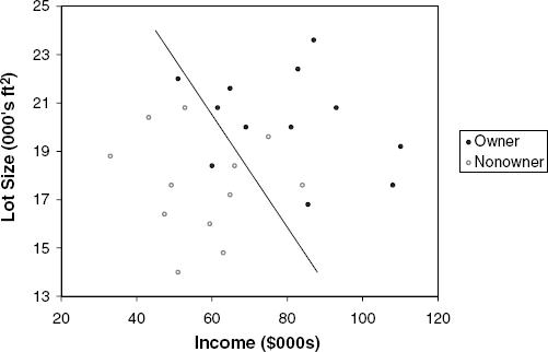
We return to the example from Chapter 7, where a riding-mower manufacturer would like to find a way of classifying families in a city into those likely to purchase a riding mower and those not likely to buy one. A pilot random sample of 12 owners and 12 nonowners in the city is undertaken. The data are given in Table 7.1, and a scatterplot is shown in Figure 12.1. We can think of a linear classification rule as a line that separates the two-dimensional region into two parts, with most of the owners in one half-plane and most nonowners in the complementary half-plane. A good classification rule would separate the data so that the fewest points are misclassified: The line shown in Figure 12.1 seems to do a good job in discriminating between the two classes as it makes 4 misclassifications out of 24 points. Can we do better?
The riding-mower example is a classic example and is useful in describing the concept and goal of discriminant analysis. However, in today's business applications, the number of records is much larger, and their separation into classes is much less distinct. To illustrate this, we return to the Universal Bank example described in Chapter 9, where the bank's goal is to find which factors make a customer more likely to accept a personal loan. For simplicity, we consider only two variables: the customer's annual income (Income, in $000s), and the average monthly credit card spending (CCAvg, in $000s). The first part of Figure 12.2 shows the acceptance of a personal loan by a subset of 200 customers from the bank's database as a function of Income and CCAvg. We use a log scale on both axes to enhance visibility because there are many points condensed in the low-income, low-CC spending area. Even for this small subset, the separation is not clear. The second figure shows all 5000 customers and the added complexity of dealing with large numbers of observations.

Finding the best separation between items involves measuring their distance from their class. The general idea is to classify an item to the class to which it is closest. Suppose that we are required to classify a new customer of Universal Bank as being an acceptor or a nonacceptor of its personal loan offer, based on an income of x. From the bank's database we find that the average income for loan acceptors was $144.75K and for nonacceptors $66.24K. We can use Income as a predictor of loan acceptance via a simple Euclidean distance rule: If x is closer to the average income of the acceptor class than to the average income of the nonacceptor class, classify the customer as an acceptor; otherwise, classify the customer as a nonacceptor. In other words, if |x − 144.75| < |x − 66.24|, classification = acceptor; otherwise, nonacceptor. Moving from a single variable (income) to two or more variables, the equivalent of the mean of a class is the centroid of a class. This is simply the vector of means
Using the Euclidean distance has three drawbacks. First, the distance depends on the units we choose to measure the variables. We will get different answers if we decide to measure income in dollars, for instance, rather than in thousands of dollars.
Second, Euclidean distance does not take into account the variability of the variables. For example, if we compare the variability in income in the two classes, we find that for acceptors the standard deviation is lower than for nonacceptors ($31.6K vs. $40.6K). Therefore, the income of a new customer might be closer to the acceptors' average income in dollars, but because of the large variability in income for nonacceptors, this customer is just as likely to be a nonacceptor. We therefore want the distance measure to take into account the variance of the different variables and measure a distance in standard deviations rather than in the original units. This is equivalent to z scores.
Third, Euclidean distance ignores the correlation between the variables. This is often a very important consideration, especially when we are using many variables to separate classes. In this case there will often be variables, which, by themselves, are useful discriminators between classes, but in the presence of other variables are practically redundant, as they capture the same effects as the other variables.
A solution to these drawbacks is to use a measure called statistical distance (or Mahalanobis distance). Let us denote by S the covariance matrix between the p variables. The definition of a statistical distance is
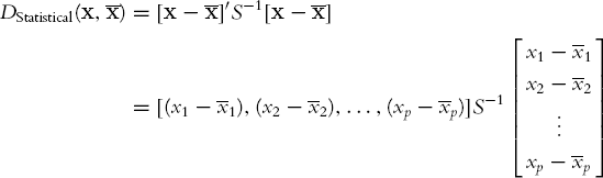
(the notation' represents transpose operation, which simply turns the column vector into a row vector). S−1 is the inverse matrix of S, which is the p-dimension extension to division. When there is a single predictor (p = 1), this reduces to a z score since we subtract the mean and divide by the standard deviation. The statistical distance takes into account not only the predictor averages but also the spread of the predictor values and the correlations between the different predictors. To compute a statistical distance between an observation and a class, we must compute the predictor averages (the centroid) and the covariances between each pair of variables. These are used to construct the distances. The method of discriminant analysis uses statistical distance as the basis for finding a separating line (or, if there are more than two variables, a separating hyperplane) that is equally distant from the different class means.[31] It is based on measuring the statistical distances of an observation to each of the classes and allocating it to the closest class. This is done through classification functions, which are explained next.
Linear classification functions were suggested in 1936 by the noted statistician R. A. Fisher as the basis for improved separation of observations into classes. The idea is to find linear functions of the measurements that maximize the ratio of between-class variability to within-class variability. In other words, we would obtain classes that are very homogeneous and differ the most from each other. For each observation, these functions are used to compute scores that measure the proximity of that observation to each of the classes. An observation is classified as belonging to the class for which it has the highest classification score (equivalent to the smallest statistical distance).
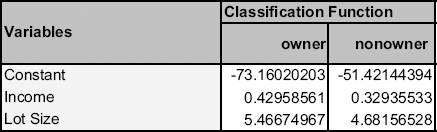
Figure 12.3. DISCRIMINANT ANALYSIS OUTPUT FOR RIDING-MOWER DATA, DISPLAYING THE ESTIMATED CLASSIFICATION FUNCTIONS
The classification functions are estimated using software (see Figure 12.3). Note that the number of classification functions is equal to the number of classes (in this case, 2).
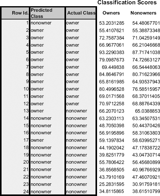
To classify a family into the class of owners or nonowners, we use the functions above to compute the family's classification scores: A family is classified into the class of owners if the owner function is higher than the nonowner function and into nonowners if the reverse is the case. These functions are specified in a way that can be generalized easily to more than two classes. The values given for the functions are simply the weights to be associated with each variable in the linear function in a manner analogous to multiple linear regression. For instance, the first household has an income of $60K and a lot size of 18.4K ft2. Their owner score is therefore −73.16 + (0.43)(60) + (5.47)(18.4) = 53.2, and their nonowner score is −51.42 + (0.33)(60) + (4.68)(18.4) = 54.48. Since the second score is higher, the household is (mis)classified by the model as a nonowner. The scores for all 24 households are given in Figure 12.4.
An alternative way for classifying an observation into one of the classes is to compute the probability of belonging to each of the classes and assigning the observation to the most likely class. If we have two classes, we need only compute a single probability for each observation (e.g., of belonging to owners). Using a cutoff of 0.5 is equivalent to assigning the observation to the class with the highest classification score. The advantage of this approach is that we can sort the records in order of descending probabilities and generate lift curves. Let us assume that there are m classes. To compute the probability of belonging to a certain class k, for a certain observation i, we need to compute all the classification scores c1(i),..., cm(i) and combine them using the following formula:
P[observation i(with measurements x1, x2, ..., xp) belongs to class k]
In XLMiner these probabilities are computed automatically, as can be seen in Figure 12.5.
We now have three misclassifications, compared to four in our original (ad hoc) classifications. This can be seen in Figure 12.6, which includes the line resulting from the discriminant model.[32]
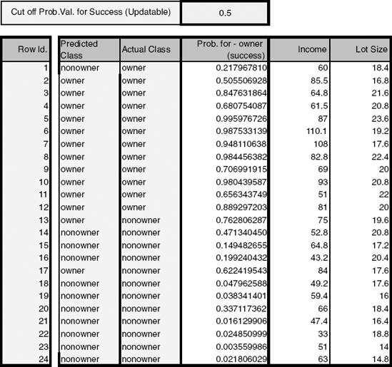
Figure 12.5. DISCRIMINANT ANALYSIS OUTPUT FOR RIDING-MOWER DATA, DISPLAYING THE ESTIMATED PROBABILITY OF OWNERSHIP FOR EACH FAMILY
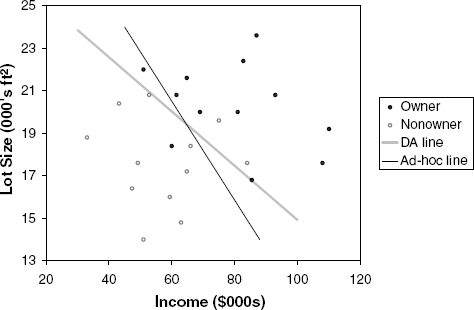
Figure 12.6. CLASS SEPARATION OBTAINED FROM THE DISCRIMINANT MODEL (COMPARED TO AD HOC LINE FROM Figure 12.1)
The discriminant analysis method relies on two main assumptions to arrive at classification scores: First, it assumes that the measurements in all classes come from a multivariate normal distribution. When this assumption is reasonably met, discriminant analysis is a more powerful tool than other classification methods, such as logistic regression. In fact, it is 30% more efficient than logistic regression if the data are multivariate normal, in the sense that we require 30% less data to arrive at the same results. In practice, it has been shown that this method is relatively robust to departures from normality in the sense that predictors can be nonnormal and even dummy variables. This is true as long as the smallest class is sufficiently large (approximately more than 20 cases). This method is also known to be sensitive to outliers in both the univariate space of single predictors and in the multivariate space. Exploratory analysis should therefore be used to locate extreme cases and determine whether they can be eliminated.
The second assumption behind discriminant analysis is that the correlation structure between the different measurements within a class is the same across classes. This can be roughly checked by estimating the correlation matrix for each class and comparing matrices. If the correlations differ substantially across classes, the classifier will tend to classify cases into the class with the largest variability. When the correlation structure differs significantly and the dataset is very large, an alternative is to use quadratic discriminant analysis.[33]
With respect to the evaluation of classification accuracy, we once again use the general measures of performance that were described in Chapter 5 (judging the performance of a classifier), with the principal ones based on the confusion matrix (accuracy alone or combined with costs) and the lift chart. The same argument for using the validation set for evaluating performance still holds. For example, in the riding-mower example, families 1, 13, and 17 are misclassified. This means that the model yields an error rate of 12.5% for these data. However, this rate is a biased estimate—it is overly optimistic because we have used the same data for fitting the classification parameters and for estimating the error. Therefore, as with all other models, we test performance on a validation set that includes data that were not involved in estimating the classification functions.
To obtain the confusion matrix from a discriminant analysis, we either use the classification scores directly or the probabilities of class membership that are computed from the classification scores. In both cases we decide on the class assignment of each observation based on the highest score or probability. We then compare these classifications to the actual class memberships of these observations. This yields the confusion matrix. In the Universal Bank case we use the estimated classification functions in Figure 12.4 to predict the probability of loan acceptance in a validation set that contains 2000 customers (these data were not used in the modeling step).
So far we have assumed that our objective is to minimize the classification error. The method presented above assumes that the chances of encountering an item from either class requiring classification is the same. If the probability of encountering an item for classification in the future is not equal for the different classes, we should modify our functions to reduce our expected (long-run average) error rate. The modification is done as follows: Let us denote by pj the prior or future probability of membership in class j (in the two-class case we have p1 and p2 = 1 − p1). We modify the classification function for each class by adding log(pj). [34] To illustrate this, suppose that the percentage of riding-mower owners in the population is 15% (compared to 50% in the sample). This means that the model should classify fewer households as owners. To account for this, we adjust the constants in the classification functions from Figure 12.3 and obtain the adjusted constants −73.16 + log(0.15) = −75.06 for owners and −51.42 + log(0.85) = −50.58 for nonowners. To see how this can affect classifications, consider family 13, which was misclassified as an owner in the case involving equal probability of class membership. When we account for the lower probability of owning a mower in the population, family 13 is classified properly as a nonowner (its owner classification score exceeds the nonowner score).
A second practical modification is needed when misclassification costs are not symmetrical. If the cost of misclassifying a class 1 item is very different from the cost of misclassifying a class 2 item, we may want to minimize the expected cost of misclassification rather than the simple error rate (which does not take cognizance of unequal misclassification costs). In the two-class case, it is easy to manipulate the classification functions to account for differing misclassification costs (in addition to prior probabilities). We denote by C1 the cost of misclassifying a class 1 member (into class 2). Similarly, C2 denotes the cost of misclassifying a class 2 member (into class 1). These costs are integrated into the constants of the classification functions by adding log(C1) to the constant for class 1 and log(C2) to the constant of class 2. To incorporate both prior probabilities and misclassification costs, add log(p1C1) to the constant of class 1 and log(p2C2) to that of class 2.
In practice, it is not always simple to come up with misclassification costs C1 and C2 for each class. It is usually much easier to estimate the ratio of costs C2/C1 (e.g., the cost of misclassifying a credit defaulter is 10 times more expensive than that of misclassifying a nondefaulter). Luckily, the relationship between the classification functions depends only on this ratio. Therefore, we can set C1 = 1 and C2 = ratio and simply add log(C2/C1) to the constant for class 2.
Ideally, every automobile accident call to 911 results in the immediate dispatch of an ambulance to the accident scene. However, in some cases the dispatch might be delayed (e.g., at peak accident hours or in some resource-strapped towns or shifts). In such cases, the 911 dispatchers must make decisions about which units to send based on sketchy information. It is useful to augment the limited information provided in the initial call with additional information in order to classify the accident as minor injury, serious injury, or death. For this purpose we can use data that were collected on automobile accidents in the United States in 2001 that involved some type of injury. For each accident, additional information is recorded, such as day of week, weather conditions, and road type. Figure 12.7 shows a small sample of records with 10 measurements of interest.
The goal is to see how well the predictors can be used to classify injury type correctly. To evaluate this, a sample of 1000 records was drawn and partitioned into training and validation sets, and a discriminant analysis was performed on the training data. The output structure is very similar to that for the two-class case. The only difference is that each observation now has three classification functions (one for each injury type), and the confusion and error matrices are 3 × 3 to account for all the combinations of correct and incorrect classifications (see Figure 12.8). The rule for classification is still to classify an observation to the class that has the highest corresponding classification score. The classification scores are computed, as before, using the classification function coefficients. This can be seen in Figure 12.9. For instance, the no injury classification score for the first accident in the training set is −24.51 + 1.95(1) + 1.19(0) + ... + 16.36(1) = 30.93. The nonfatal score is similarly computed as 31.42 and the fatal score as 25.94. Since the nonfatal score is highest, this accident is (correctly) classified as having nonfatal injuries.
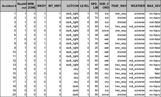
Figure 12.7. SAMPLE OF 20 AUTOMOBILE ACCIDENTS FROM THE 2001 DEPARTMENT OF TRANSPORTATION DATABASE. EACH ACCIDENT IS CLASSIFIED AS ONE OF THREE INJURY TYPES (NO INJURY, NONFATAL, OR FATAL) AND HAS 10 MEASUREMENTS (EXTRACTED FROM A LARGER SET OF MEASUREMENTS)
We can also compute for each accident the estimated probabilities of belonging to each of the three classes using the same relationship between classification scores and probabilities as in the two-class case. For instance, the probability of the above accident involving nonfatal injuries is estimated by the model as
The probabilities of an accident involving no injuries or fatal injuries are computed in a similar manner. For the first accident in the training set, the highest probability is that of involving no injuries, and therefore it is classified as a no injury accident. In general, membership probabilities can be obtained directly from XLMiner for the training set, the validation set, or for new observations.
Discriminant analysis tends to be considered more of a statistical classification method than a data mining method. This is reflected in its absence or short mention in many data mining resources. However, it is very popular in social sciences and has shown good performance. The use and performance of discriminant analysis are similar to those of multiple linear regression. The two methods therefore share several advantages and weaknesses.
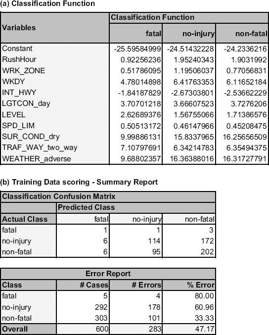
Figure 12.8. XLMINER'S DISCRIMINANT ANALYSIS OUTPUT FOR THE THREE-CLASS INJURY EXAMPLE: (A) CLASSIFICATION FUNCTIONS AND (B) CONFUSION MATRIX FOR TRAINING SET
Like linear regression, discriminant analysis searches for the optimal weighting of predictors. In linear regression the weighting is with relation to the response, whereas in discriminant analysis it is with relation to separating the classes. Both use the same estimation method of least squares, and the resulting estimates are robust to local optima.
In both methods an underlying assumption is normality. In discriminant analysis we assume that the predictors are approximately from a multivariate normal distribution. Although this assumption is violated in many practical situations (such as with commonly used binary predictors), the method is surprisingly robust. According to Hastie et al. (2001), the reason might be that data can usually support only simple separation boundaries, such as linear boundaries. However, for continuous variables that are found to be very skewed (e.g., through a histogram), transformations such as the log transform can improve performance. In addition, the method's sensitivity to outliers commands exploring the data for extreme values and removing those records from the analysis.
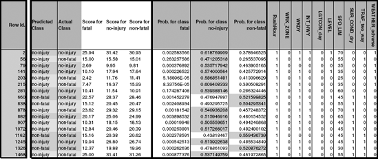
Figure 12.9. CLASSIFICATION SCORES, MEMBERSHIP PROBABILITIES, AND CLASSIFICATIONS FOR THE THREE-CLASS INJURY TRAINING DATASET.
An advantage of discriminant analysis as a classifier (it is like logistic regression in this respect) is that it provides estimates of single-predictor contributions. This is useful for obtaining a ranking of the importance of predictors, and for variable selection.
Finally, the method is computationally simple, parsimonious, and especially useful for small datasets. With its parametric form, discriminant analysis makes the most out of the data and is therefore especially useful where the data are few (as explained in Section 12.4).
Personal Loan Acceptance. Universal Bank is a relatively young bank growing rapidly in terms of overall customer acquisition. The majority of these customers are liability customers with varying sizes of relationship with the bank. The customer base of asset customers is quite small, and the bank is interested in expanding this base rapidly to bring in more loan business. In particular, it wants to explore ways of converting its liability customers to personal loan customers.
A campaign the bank ran for liability customers last year showed a healthy conversion rate of over 9% successes. This has encouraged the retail marketing department to devise smarter campaigns with better target marketing. The goal of our analysis is to model the previous campaign's customer behavior to analyze what combination of factors make a customer more likely to accept a personal loan. This will serve as the basis for the design of a new campaign.
The file UniversalBank.xls contains data on 5000 customers. The data include customer demographic information (e.g., age, income), the customer's relationship with the bank (e.g., mortgage, securities account), and the customer response to the last personal loan campaign (Personal Loan). Among these 5000 customers, only 480 (= 9.6%) accepted the personal loan that was offered to them in the previous campaign.
Partition the data (60% training and 40% validation) and then perform a discriminant analysis that models Personal Loan as a function of the remaining predictors (excluding zip code). Remember to turn categorical predictors with more than two categories into dummy variables first. Specify the success class as 1 (loan acceptance), and use the default cutoff value of 0.5.
Compute summary statistics for the predictors separately for loan acceptors and nonacceptors. For continuous predictors, compute the mean and standard deviation. For categorical predictors, compute the percentages. Are there predictors where the two classes differ substantially?
Examine the model performance on the validation set.
What is the misclassification rate?
Is one type of misclassification more likely than the other?
Select three customers who were misclassified as acceptors and three who were misclassified as nonacceptors. The goal is to determine why they are misclassified. First, examine their probability of being classified as acceptors: Is it close to the threshold of 0.5? If not, compare their predictor values to the summary statistics of the two classes to determine why they were misclassified.
As in many marketing campaigns, it is more important to identify customers who will accept the offer rather than customers who will not accept it. Therefore, a good model should be especially accurate at detecting acceptors. Examine the lift chart and decile chart for the validation set and interpret them in light of this goal.
Compare the results from the discriminant analysis with those from a logistic regression (both with cutoff 0.5 and the same predictors). Examine the confusion matrices, the lift charts, and the decile charts. Which method performs better on your validation set in detecting the acceptors?
The bank is planning to continue its campaign by sending its offer to 1000 additional customers. Suppose that the cost of sending the offer is $1 and the profit from an accepted offer is $50. What is the expected profitability of this campaign?
The cost of misclassifying a loan acceptor customer as a nonacceptor is much higher than the opposite misclassification cost. To minimize the expected cost of misclassification, should the cutoff value for classification (which is currently at 0.5) be increased or decreased?
Identifying Good System Administrators. A management consultant is studying the roles played by experience and training in a system administrator's ability to complete a set of tasks in a specified amount of time. In particular, she is interested in discriminating between administrators who are able to complete given tasks within a specified time and those who are not. Data are collected on the performance of 75 randomly selected admin istrators. They are stored in the file SystemAdministrators.xls.
Using these data, the consultant performs a discriminant analysis. The variable Experience measures months of full-time system administrator experience, while Training measures number of relevant training credits. The dependent variable Completed is either Yes or No, according to whether or not the administrator completed the tasks.
Create a scatterplot of Experience versus Training using color or symbol to differentiate administrators who completed the tasks from those who did not complete them. See if you can identify a line that separates the two classes with minimum misclassification.
Run a discriminant analysis with both predictors using the entire dataset as training data. Among those who completed the tasks, what is the percentage of administrators who are classified incorrectly as failing to complete the tasks?
Compute the two classification scores for an administrator with 4 years of higher education and 6 credits of training. Based on these, how would you classify this administrator?
How much experience must be accumulated by a administrator with 4 training credits before his or her estimated probability of completing the tasks exceeds 50%?
Compare the classification accuracy of this model to that resulting from a logistic regression with cutoff 0.5.
Compute the correlation between Experience and Training for administrators that completed the tasks and compare it to the correlation of administrators who did not complete the tasks. Does the equal correlation assumption seem reasonable?
Detecting Spam E-mail (from the UCI Machine Learning Repository). A team at Hewlett-Packard collected data on a large number of e-mail messages from their post master and personal e-mail for the purpose of finding a classifier that can separate e-mail messages that are spam versus nonspam (a.k.a. "ham"). The spam concept is diverse: It includes advertisements for products or websites, "make money fast" schemes, chain letters, pornography, and so on. The definition used here is "unsolicited commercial e-mail." The file Spambase.xls contains information on 4601 e-mail messages, among which 1813 are tagged "spam." The predictors include 57 attributes, most of them are the average number of times a certain word (e.g., mail, George) or symbol (e.g., #, !) appears in the e-mail. A few predictors are related to the number and length of capitalized words.
To reduce the number of predictors to a manageable size, examine how each predictor differs between the spam and nonspam e-mails by comparing the spam-class average and nonspam-class average. Which are the 11 predictors that appear to vary the most between spam and nonspam e-mails? From these 11, which words or signs occur more often in spam?
Partition the data into training and validation sets; then perform a discriminant analysis on the training data using only the 11 predictors.
If we are interested mainly in detecting spam messages, is this model useful? Use the confusion matrix, lift chart, and decile chart for the validation set for the evaluation.
In the sample, almost 40% of the e-mail messages were tagged as spam. However, suppose that the actual proportion of spam messages in these e-mail accounts is 10%. Compute the constants of the classification functions to account for this information.
A spam filter that is based on your model is used, so that only messages that are classified as nonspam are delivered, while messages that are classified as spam are quarantined. In this case, misclassifying a nonspam e-mail (as spam) has much heftier results. Suppose that the cost of quarantining a nonspam e-mail is 20 times that of not detecting a spam message. Compute the constants of the classification functions to account for these costs (assume that the proportion of spam is reflected correctly by the sample proportion).
[30] Data Mining for Business Intelligence, By Galit Shmueli, Nitin R. Patel, and Peter C. Bruce
[31] An alternative approach finds a separating line or hyperplane that is "best" at separating the different clouds of points. In the case of two classes, the two methods coincide.
[32] The slope of the line is given by -a1/a2 and the intercept is
[33] In practice, quadratic discriminant analysis has not been found useful except when the difference in the correlation matrices is large and the number of observations available for training and testing is large. The reason is that the quadratic model requires estimating many more parameters that are all subject to error [for c classes and p variables, the total number of parameters to be estimated for all the different correlation matrices is cp (p + 1)/2].
[34] XLMiner also has the option to set the prior probabilities as the ratios that are encountered in the dataset. This is based on the assumption that a random sample will yield a reasonable estimate of membership probabilities. However, for other prior probabilities the classification functions should be modified manually.