In this chapter we describe the unsupervised learning methods of association rules (also called "affinity analysis"), where the goal is to identify item clusterings in transaction-type databases. Association rule discovery is popular in marketing, where it is called "market basket analysis" and is aimed at discovering which groups of products tend to be purchased together. We describe the two-stage process of rule generation and then assessment of rule strength to choose a subset. We describe the popular rule-generating Apriori algorithm and then criteria for judging the strength of rules. We also discuss issues related to the required data format and nonautomated methods for condensing the list of generated rules. The entire process is illustrated in a numerical example.
Put simply, association rules, or affinity analysis, constitute a study of "what goes with what." For example, a medical researcher wants to learn what symptoms go with what confirmed diagnoses. This method is also called market basket analysis because it originated with the study of customer transactions databases to determine dependencies between purchases of different items.
The availability of detailed information on customer transactions has led to the development of techniques that automatically look for associations between items that are stored in the database. An example is data collected using bar code scanners in supermarkets. Such market basket databases consist of a large number of transaction records. Each record lists all items bought by a customer on a single-purchase transaction. Managers would be interested to know if certain groups of items are consistently purchased together. They could use these data for store layouts to place items optimally with respect to each other, or they could use such information for cross selling, for promotions, for catalog design, and to identify customer segments based on buying patterns. Association rules provide information of this type in the form of "if—then" statements. These rules are computed from the data; unlike the if—then rules of logic, association rules are probabilistic in nature.
Such rules are commonly encountered in online recommendation systems(or recommender systems), where customers examining an item or items for possible purchase are shown other items that are often purchased in conjunction with the first item(s). The display from Amazon.com's online shopping system illustrates the application of rules such as this. In the example shown in Figure 13.1 a purchaser of Last Train Homeo's Bound Away audio CD is shown the other CDs most frequently purchased by other Amazon purchasers of this CD.

Table 13.1. TRANSACTIONS FOR PURCHASES OF DIFFERENT-COLORED CELLULAR PHONE FACEPLATES
Transaction | Faceplate | Colors | Purchases | |
|---|---|---|---|---|
1 | red | white | green | |
2 | white | orange | ||
3 | white | blue | ||
4 | red | white | orange | |
5 | red | blue | ||
6 | white | blue | ||
7 | white | orange | ||
8 | red | white | blue | green |
9 | red | white | blue | |
10 | yellow |
We introduce a simple artificial example and use it throughout the chapter to demonstrate the concepts, computations, and steps of affinity analysis. We end by applying affinity analysis to a more realistic example of book purchases.
A store that sells accessories for cellular phones runs a promotion on faceplates. Customers who purchase multiple faceplates from a choice of six different colors get a discount. The store managers, who would like to know what colors of faceplates customers are likely to purchase together, collected the transaction database as shown in Table 13.1.
The idea behind association rules is to examine all possible rules between items in an if–then format and select only those that are most likely to be indicators of true dependence. We use the term antecedent to describe the "if" part, and consequent to describe the "then" part. In association analysis, the antecedent and consequent are sets of items (called item sets) that are disjoint (do not have any items in common).
Returning to the phone faceplate purchase example, one example of a possible rule is "if red, then white," meaning that if a red faceplate is purchased, a white one is, too. Here the antecedent is red and the consequent is white. The antecedent and consequent each contain a single item in this case. Another possible rule is "if red and white, then green." Here the antecedent includes the item set {red, white} and the consequent is {green}.
The first step in affinity analysis is to generate all the rules that would be candidates for indicating associations between items. Ideally, we might want to look at all possible combinations of items in a database with p distinct items (in the phone faceplate example, p = 6). This means finding all combinations of single items, pairs of items, triplets of items, and so on in the transactions database. However, generating all these combinations requires a long computation time that grows exponentially in k. A practical solution is to consider only combinations that occur with higher frequency in the database. These are called frequent item sets.
Determining what consists of a frequent item set is related to the concept of support. The support of a rule is simply the number of transactions that include both the antecedent and consequent item sets. It is called a support because it measures the degree to which the data "support" the validity of the rule. The support is sometimes expressed as a percentage of the total number of records in the database. For example, the support for the item set {red,white}in the phone faceplate example is 4 (100 x 140= 40%).
What constitutes a frequent item set is therefore defined as an item set that has a support that exceeds a selected minimum support, determined by the user.
Several algorithms have been proposed for generating frequent item sets, but the classic algorithm is the Apriori algorithm of Agrawal et al. (1993). The key idea of the algorithm is to begin by generating frequent item sets with just one item (one-item sets) and to recursively generate frequent item sets with two items, then with three items, and so on until we have generated frequent item sets of all sizes.
It is easy to generate frequent one-item sets. All we need to do is to count, for each item, how many transactions in the database include the item. These transaction counts are the supports for the one-item sets. We drop one-item sets that have support below the desired minimum support to create a list of the frequent one-item sets.
To generate frequent two-item sets, we use the frequent one-item sets. The reasoning is that if a certain one-item set did not exceed the minimum support, any larger size item set that includes it will not exceed the minimum support. In general, generating k-item sets uses the frequent (k – 1)-item sets that were generated in the preceding step. Each step requires a single run through the database, and therefore the Apriori algorithm is very fast even for a large number of unique items in a database.
From the abundance of rules generated, the goal is to find only the rules that indicate a strong dependence between the antecedent and consequent item sets. To measure the strength of association implied by a rule, we use the measures of confidence and lift ratio, as described below.
In addition to support, which we described earlier, there is another measure that expresses the degree of uncertainty about the if—then rule. This is known as the confidence[36] of the rule. This measure compares the co-occurrence of the antecedent and consequent item sets in the database to the occurrence of the antecedent item sets. Confidence is defined as the ratio of the number of transactions that include all antecedent and consequent item sets (namely, the support) to the number of transactions that include all the antecedent item sets:
For example, suppose that a supermarket database has 100,000 point-of-sale transactions. Of these transactions, 2000 include both orange juice and (over-the-counter) flu medication, and 800 of these include soup purchases. The association rule "IF orange juice and flu medication are purchased THEN soup is purchased on the same trip" has a support of 800 transactions (alternatively, 0.8% = 800/100,000) and a confidence of 40% (= 800/2000).
To see the relationship between support and confidence, let us think about what each is measuring (estimating). One way to think of support is that it is the (estimated) probability that a transaction selected randomly from the database will contain all items in the antecedent and the consequent:
In comparison, the confidence is the (estimated) conditional probability that a transaction selected randomly will include all the items in the consequent given that the transaction includes all the items in the antecedent:
A high value of confidence suggests a strong association rule (in which we are highly confident). However, this can be deceptive because if the antecedent and/or the consequent has a high level of support, we can have a high value for confidence even when the antecedent and consequent are independent! For example, if nearly all customers buy bananas and nearly all customers buy ice cream, the confidence level will be high regardless of whether there is an association between the items.
A better way to judge the strength of an association rule is to compare the confidence of the rule with a benchmark value, where we assume that the occurrence of the consequent item set in a transaction is independent of the occurrence of the antecedent for each rule. In other words, if the antecedent and consequent item sets are independent, what confidence values would we expect to see? Under independence, the support would be
and the benchmark confidence would be
The estimate of this benchmark from the data, called the benchmark confidence value for a rule, is computed by
We compare the confidence to the benchmark confidence by looking at their ratio: This is called the lift ratio of a rule. The lift ratio is the confidence of the rule divided by the confidence, assuming independence of consequent from antecedent:
A lift ratio greater than 1.0 suggests that there is some usefulness to the rule. In other words, the level of association between the antecedent and consequent item sets is higher than would be expected if they were independent. The larger the lift ratio, the greater the strength of the association.
To illustrate the computation of support, confidence, and lift ratio for the cellular phone faceplate example, we introduce a presentation of the data better suited to this purpose.
Transaction data are usually displayed in one of two formats: a list of items purchased (each row representing a transaction), or a binary matrix in which columns are items, rows again represent transactions, and each cell has either a 1 or a 0, indicating the presence or absence of an item in the transaction. For example, Table 13.1 displays the data for the cellular faceplate purchases in item list format. We translate these into binary matrix format in Table 13.2.
Table 13.2. PHONE FACEPLATE DATE IN BINARY MATRIX FORMAT
Transaction | Red | White | Blue | Orange | Green | Yellow |
|---|---|---|---|---|---|---|
1 | 1 | 1 | 0 | 0 | 1 | 0 |
2 | 0 | 1 | 0 | 1 | 0 | 0 |
3 | 0 | 1 | 1 | 0 | 0 | 0 |
4 | 1 | 1 | 0 | 1 | 0 | 0 |
5 | 1 | 0 | 1 | 0 | 0 | 0 |
6 | 0 | 1 | 1 | 0 | 0 | 0 |
7 | 1 | 0 | 1 | 0 | 0 | 0 |
8 | 1 | 1 | 1 | 0 | 1 | 0 |
9 | 1 | 1 | 1 | 0 | 0 | 0 |
10 | 0 | 0 | 0 | 0 | 0 | 1 |
Now suppose that we want association rules between items for this database that have a support count of at least 2 (equivalent to a percentage support of 2/10 = 20%): in other words, rules based on items that were purchased together in at least 20% of the transactions. By enumeration, we can see that only the item sets listed in Table 13.3 have a count of at least 2.
Table 13.3. ITEM SETS WITH SUPPORT COUNT OF AT LEAST TWO
Item Set | Support (Count) |
|---|---|
{red} | 6 |
{white} | 7 |
{blue} | 6 |
{orange} | 2 |
{green} | 2 |
{red, white} | 4 |
{red, blue} | 4 |
{red, green} | 2 |
{white, blue} | 4 |
{white, orange} | 2 |
{white, green} | 2 |
{red, white, blue} | 2 |
{red, white, green} | 2 |
The first item set {red}has a support of 6 because six of the transactions included a red faceplate. Similarly, the last item set {red, white, green}has a support of 2 because only two transactions included red, white, and green faceplates.
Note
In XLMiner the user can choose to input data using the Affinity> Association Rules facility in either item list format or binary matrix format.
The process of selecting strong rules is based on generating all association rules that meet stipulated support and confidence requirements. This is done in two stages. The first stage, described in Section 13.3, consists of finding all "frequent" item sets, those item sets that have a requisite support. In the second stage we generate, from the frequent item sets, association rules that meet a confidence requirement. The first step is aimed at removing item combinations that are rare in the database. The second stage then filters the remaining rules and selects only those with high confidence. For most association analysis data, the computational challenge is the first stage, as described in the discussion of the Apriori algorithm.
The computation of confidence in the second stage is simple. Since any subset (e.g., {red}in the phone faceplate example) must occur at least as frequently as the set it belongs to (e.g., {red, white}), each subset will also be in the list. It is then straightforward to compute the confidence as the ratio of the support for the item set to the support for each subset of the item set. We retain the corresponding association rule only if it exceeds the desired cutoff value for confidence. For example, from the item set {red, white, green}in the phone faceplate purchases, we get the following association rules:


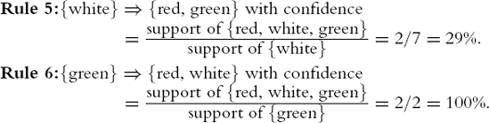
If the desired minimum confidence is 70%, we would report only the second, third, and last rules.
We can generate association rules in XLMiner by specifying the minimum support count (2) and minimum confidence level percentage (70%). Figure 13.2 shows the output. Note that here we consider all possible item sets, not just { red, white, green}as above.
The output includes information on the support of the antecedent, the support of the consequent, and the support of the combined set [denoted by Support (aU c)]. It also gives the confidence of the rule (in percent) and the lift ratio. In addition, XLMiner has an interpreter that translates the rule from a certain row into English. In the snapshot shown in Figure 13.2, the first rule is highlighted (by clicking), and the corresponding English rule appears in the yellow box:
Rule 1: If item(s) green= is/are purchased, then this implies item(s) red, white is/are also purchased. This rule has confidence of 100%.
In interpreting results, it is useful to look at the various measures. The support for the rule indicates its impact in terms of overall size: What proportion of transactions is affected? If only a small number of transactions are affected, the rule may be of little use (unless the consequent is very valuable and/or the rule is very efficient in finding it).
The lift ratio indicates how efficient the rule is in finding consequents, compared to random selection. A very efficient rule is preferred to an inefficient rule, but we must still consider support: A very efficient rule that has very low support may not be as desirable as a less efficient rule with much greater support.
The confidence tells us at what rate consequents will be found and is useful in determining the business or operational usefulness of a rule: A rule with low confidence may find consequents at too low a rate to be worth the cost of (say) promoting the consequent in all the transactions that involve the antecedent.
What about confidence in the nontechnical sense? How sure can we be that the rules we develop are meaningful? Considering the matter from a statistical perspective, we can ask: Are we finding associations that are really just chance occurrences?
Let us examine the output from an application of this algorithm to a small database of 50 transactions, where each of the 9 items is assigned randomly to each transaction. The data are shown in Table 13.4, and the association rules generated are shown in Table 13.5.
Table 13.4. FIFTY TRANSACTION OF RANDOMLY ASSIGNED ITEMS
Transaction | Items | Transaction | Items | Transaction | Items |
|---|---|---|---|---|---|
1 | 8 | 18 | 8 | 35 | 3 4 6 8 |
2 | 3 4 8 | 19 | 36 | 1 4 8 | |
3 | 8 | 20 | 9 | 37 | 4 7 8 |
4 | 3 9 | 21 | 2 5 6 8 | 38 | 8 9 |
5 | 9 | 22 | 4 6 9 | 39 | 4 5 7 9 |
6 | 1 8 | 23 | 4 9 | 40 | 2 8 9 |
7 | 6 9 | 24 | 8 9 | 41 | 2 5 9 |
8 | 3 5 7 9 | 25 | 6 8 | 42 | 1 2 7 9 |
9 | 8 | 26 | 1 6 8 | 43 | 5 8 |
10 | 27 | 5 8 | 44 | 1 7 8 | |
11 | 1 7 9 | 28 | 4 8 9 | 45 | 8 |
12 | 1 4 5 8 9 | 29 | 9 | 46 | 2 7 9 |
13 | 5 7 9 | 30 | 8 | 47 | 4 6 9 |
14 | 6 7 8 | 31 | 1 5 8 | 48 | 9 |
15 | 3 7 9 | 32 | 3 6 9 | 49 | 9 |
16 | 1 4 9 | 33 | 7 9 | 50 | 6 7 8 |
17 | 6 7 8 | 34 | 7 8 9 |
Table 13.5. ASSOCIATION RULES OUTPUT FOR RANDOM DATA
|
Min. Support: 2 = 4% Min. Conf. % : 70 | |||||||||
|---|---|---|---|---|---|---|---|---|---|
Rule | Confidence (%) | Anteced., a | Conseq., c | Support (a) | Support (c) | Support (a U c) | Confidence If P(c|a)= P(c) (%) | Lift Ratio (conf./ prev.col.) | |
1 | 80 | 2 | ⇒ | 9 | 5 | 27 | 4 | 54 | 1.5 |
2 | 100 | 5.7 | ⇒ | 9 | 3 | 27 | 3 | 54 | 1.9 |
3 | 100 | 6.7 | ⇒ | 8 | 3 | 29 | 3 | 58 | 1.7 |
4 | 100 | 1,5 | ⇒ | 8 | 2 | 29 | 2 | 58 | 1.7 |
5 | 100 | 2,7 | ⇒ | 9 | 2 | 27 | 2 | 54 | 1.9 |
6 | 100 | 3,8 | ⇒ | 4 | 2 | 11 | 2 | 22 | 4.5 |
7 | 100 | 3,4 | ⇒ | 8 | 2 | 29 | 2 | 58 | 1.7 |
8 | 100 | 3,7 | ⇒ | 9 | 2 | 27 | 2 | 547 | 1.9 |
9 | 100 | 4,5 | ⇒ | 9 | 2 | 27 | 2 | 54 | 1.9 |
In this example, the lift ratios highlight rule 6 as most interesting, as it suggests that purchase of item 4 is almost five times as likely when items 3 and 8 are purchased than if item 4 was not associated with the item set {3,8}. Yet we know there is no fundamental association underlying these data–they were generated randomly.
Two principles can guide us in assessing rules for possible spuriousness due to chance effects:
The more records the rule is based on, the more solid the conclusion. The key evaluative statistics are based on ratios and proportions, and we can look to statistical confidence intervals on proportions, such as political polls, for a rough preliminary idea of how variable rules might be owing to chance sampling variation. Polls based on 1500 respondents, for example, yield margins of error in the range of ±1.5%.
The more distinct rules we consider seriously (perhaps consolidating multiple rules that deal with the same items), the more likely it is that at least some will be based on chance sampling results. For one person to toss a coin 10 times and get 10 heads would be quite surprising. If 1000 people toss a coin 10 times apiece, it would not be nearly so surprising to have one get 10 heads. Formal adjustment of "statistical significance" when multiple comparisons are made is a complex subject in its own right and beyond the scope of this book. A reasonable approach is to consider rules from the top down in terms of business or operational applicability and not consider more than can reasonably be incorporated in a human decision-making process. This will impose a rough constraint on the dangers that arise from an automated review of hundreds or thousands of rules in search of "something interesting."
We now consider a more realistic example, using a larger database and real transactional data.
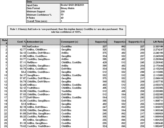
The following example (drawn from the Charles Book Club case) examines associations among transactions involving various types of books. The database includes 2000 transactions, and there are 11 different types of books. The data, in binary matrix form, are shown in Figure 13.3. For instance, the first transaction included YouthBks (youth books), DoItYBks (do-it-yourself books), and GeogBks (geography books). Figure 13.4 shows (part of) the rules generated by XLMiner's Association Rules on these data. We specified a minimal support of 200 transactions and a minimal confidence of 50%. This resulted in 49 rules (the first 26 rules are shown in Figure 13.4.
In reviewing these rules, we can see that the information can be compressed. First, rule 1, which appears from the confidence level to be a very promising rule, is probably meaningless. It says: "If Italian cooking books have been purchased, then cookbooks are purchased." It seems likely that Italian cooking books are simply a subset of cookbooks. Rules 2 and 7 involve the same trio of books, with different antecedents and consequents. The same is true of rules 14 and 15 and rules 9 and 10. (Pairs and groups like this are easy to track down by looking for rows that share the same support.) This does not mean that the rules are not useful. On the contrary, it can reduce the number of item sets to be considered for possible action from a business perspective.

Affinity analysis (also called market basket analysis) is a method for deducing rules on associations between purchased items from databases of transactions. The main advantage of this method is that it generates clear, simple rules of the form "IF X is purchased THEN Y is also likely to be purchased." The method is very transparent and easy to understand.
The process of creating association rules is two staged. First, a set of candidate rules based on frequent item sets is generated (the Apriori algorithm being the most popular rule-generating algorithm). Then from these candidate rules, the rules that indicate the strongest association between items are selected. We use the measures of support and confidence to evaluate the uncertainty in a rule. The user also specifies minimal support and confidence values to be used in the rule generation and selection process. A third measure, the lift ratio, compares the efficiency of the rule to detect a real association compared to a random combination.
One shortcoming of association rules is the profusion of rules that are generated. There is therefore a need for ways to reduce these to a small set of useful and strong rules. An important nonautomated method to condense the information involves examining the rules for noninformative and trivial rules as well as for rules that share the same support.
Another issue that needs to be kept in mind is that rare combinations tend to be ignored because they do not meet the minimum support requirement. For this reason it is better to have items that are approximately equally frequent in the data. This can be achieved by using higher level hierarchies as the items. An example is to use types of audio CDs rather than names of individual audio CDs in deriving association rules from a database of music store transactions.
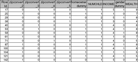
13.1 Satellite Radio Customers. An analyst at a subscription-based satellite radio company has been given a sample of data from their customer database, with the goal of finding groups of customers that are associated with one another. The data consist of company data, together with purchased demographic data that are mapped to the company data (see Figure 13.5). The analyst decides to apply association rules to learn more about the associations between customers. Comment on this approach.
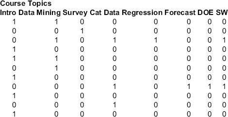
13.2 Online Statistics Courses. Consider the data in the file CourseTopics.xls, the first few rows of which are shown in Figure 13.6. These data are for purchases of online statistics courses at
statistics.com. Each row represents the courses attended by a single customer.The firm wishes to assess alternative sequencings and combinations of courses. Use association rules to analyze these data and interpret several of the resulting rules.
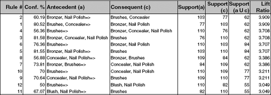
13.3 Cosmetics Purchases. The data shown in Figure 13.7 are a subset of a dataset on cosmetic purchases given in binary matrix form. The complete dataset (in the file Cosmetics.xls) contains data on the purchases of different cosmetic items at a large chain drugstore. The store wants to analyze associations among purchases of these items for purposes of point-of-sale display, guidance to sales personnel in promoting cross sales, and guidance for piloting an eventual time-of-purchase electronic recommender system to boost cross sales. Consider first only the subset shown in Figure 13.7.
Select several values in the matrix and explain their meaning.
Consider the results of the association rules analysis shown in Figure 13.8 and:
For the first row, explain the "Conf. %" output and how it is calculated.
For the first row, explain the "Support(a)," "Support(c)," and "Support(a c)" output and how it is calculated.
For the first row, explain the "Lift Ratio" and how it is calculated.
For the first row, explain the rule that is represented there in words. Now, use the complete dataset on the cosmetics purchases (in the file Cosmet-ics.xls).
Using XLMiner, apply association rules to these data.
Interpret the first three rules in the output in words.
Reviewing the first couple of dozen rules, comment on their redundancy and how you would assess their utility.