
In this chapter we describe neural nets, a flexible data-driven method that can be used for classification or prediction. Although considered a "blackbox" in terms of interpretability, neural nets have been highly successful in terms of predictive accuracy. We discuss the concepts of "nodes" and "layers" (input layers, output layers, and hidden layers) and how they connect to form the structure of a network. We then explain how a neural network is fitted to data using a numerical example. Because overfitting is a major danger with neural nets, we present a strategy for avoiding it. We describe the different parameters that a user must specify and explain the effect of each on the process. Finally, we discuss the usefulness of neural nets and their limitations.
Neural networks, also called artificial neural networks, are models for classification and prediction. The neural network is based on a model of biological activity in the brain, where neurons are interconnected and learn from experience. Neural networks mimic the way that human experts learn. The learning and memory properties of neural networks resemble the properties of human learning and memory, and they also have a capacity to generalize from particulars.
A number of successful applications have been reported in financial applications [see Trippi and Turban, (1996)] such as bankruptcy predictions, currency market trading, picking stocks and commodity trading, detecting fraud in credit card and monetary transactions, and customer relationship management (CRM). There have also been a number of very successful applications of neural nets in engineering applications. One of the best known is ALVINN, an autonomous vehicle driving application for normal speeds on highways. Using as input a 30 × 32 grid of pixel intensities from a fixed camera on the vehicle, the classifier provides the direction of steering. The response variable is a categorical one with 30 classes, such as sharp left, straight ahead, and bear right.
The main strength of neural networks is their high predictive performance. Their structure supports capturing very complex relationships between predictors and a response, which is often not possible with other classifiers.
The idea behind neural networks is to combine the input information in a very flexible way that captures complicated relationships among these variables and between them and the response variable. For instance, recall that in linear regression models the form of the relationship between the response and the predictors is assumed to be linear. In many cases the exact form of the relationship is much more complicated or is generally unknown. In linear regression modeling we might try different transformations of the predictors, interactions between predictors, and so on. In comparison, in neural networks the user is not required to specify the correct form. Instead, the network tries to learn about such relationships from the data. In fact, linear regression and logistic regression can be thought of as special cases of very simple neural networks that have only input and output layers and no hidden layers.
Although researchers have studied numerous different neural network architectures, the most successful applications in data mining of neural networks have been multilayer feedforward networks. These are networks in which there is an input layer consisting of nodes that simply accept the input values and successive layers of nodes that receive input from the previous layers. The outputs of nodes in a layer are inputs to nodes in the next layer. The last layer is called the output layer. Layers between the input and output layers are known as hidden layers. A feedforward network is a fully connected network with a one-way flow and no cycles. Figure 11.1 shows a diagram for this architecture (two hidden layers are shown in this example).
To illustrate how a neural network is fitted to data, we start with a very small illustrative example. Although the method is by no means operational in such a small example, it is useful for explaining the main steps and operations, for showing how computations are done, and for integrating all the different aspects of neural network data fitting. We later discuss a more realistic setting.

Consider the following very small dataset. Table 11.1 includes information on a tasting score for a certain processed cheese. The two predictors are scores for fat and salt, indicating the relative presence of fat and salt in the particular cheese sample (where 0 is the minimum amount possible in the manufacturing process and 1 the maximum). The output variable is the cheese sample's consumer taste acceptance, where 1 indicates that a taste test panel likes the cheese and 0 that it does not like it.
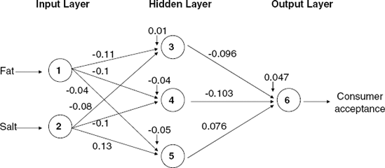
Figure 11.2 describes an example of a typical neural net that could be used for predicting the acceptance for these data. We numbered the nodes in the example from 1 to 6. Nodes 1 and 2 belong to the input layer, nodes 3-5 belong to the hidden layer, and node 6 belongs to the output layer. The values on the connecting arrows are called weights, and the weight on the arrow from node i to node j is denoted by wij. The additional bias nodes, denoted by θj, serve as an intercept for the output from node j. These are all explained in further detail below.

We discuss the input and output of the nodes separately for each of the three types of layers (input, hidden, and output). The main difference is the function used to map from the input to the output of the node.
Input nodes take as input the values of the predictors. Their output is the same as the input. If we have p predictors, the input layer will usually include p nodes. In our example there are two predictors, and therefore the input layer (shown in Figure 11.2) includes two nodes, each feeding into each node of the hidden layer. Consider the first observation: The input into the input layer is fat = 0.2 and salt = 0.9, and the output of this layer is also x1 = 0.2 and x2 = 0.9.
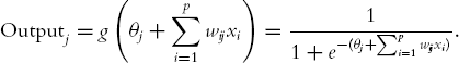
Hidden layer nodes take as input the output values from the input layer. The hidden layer in this example consists of three nodes, each receiving input from all the input nodes. To compute the output of a hidden layer node, we compute a weighted sum of the inputs and apply a certain function to it. More formally, for a set of input values x1, x2, . . ., xp, we compute the output of node j by taking the weighted sum[29]
If we use a logistic function, we can write the output of node j in the hidden layer as
Initializing the Weights The values of θj and wij are typically initialized to small (generally random) numbers in the range 0.00 ± 0.05. Such values represent a state of no knowledge by the network, similar to a model with no predictors. The initial weights are used in the first round of training.
Returning to our example, suppose that the initial weights for node 3 are θ3= −0.3, w1,3 = 0.05, and w2,3 = 0.01 (as shown in Figure 11.3). Using the logistic function, we can compute the output of node 3 in the hidden layer (using the first observation) as
Figure 11.3 shows the initial weights, inputs, and outputs for observation 1 in our tiny example. If there is more than one hidden layer, the same calculation applies, except that the input values for the second, third, and so on hidden layers would be the output of the preceding hidden layer. This means that the number of input values into a certain node is equal to the number of nodes in the preceding layer. (If there was an additional hidden layer in our example, its nodes would receive input from the three nodes in the first hidden layer.)
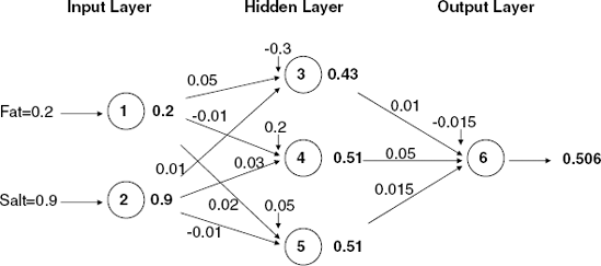
Figure 11.3. COMPUTING NODE OUTPUTS (IN BOLDFACE TYPE) USING THE FIRST OBSERVATION IN THE TINY EXAMPLE AND A LOGISTIC FUNCTION
Finally, the output layer obtains input values from the (last) hidden layer. It applies the same function as above to create the output. In other words, it takes a weighted average of its input values and then applies the function g. This is the prediction of the model. For classification we use a cutoff value (for a binary response) or the output node with the largest value (for more than two classes).
Returning to our example, the single output node (node 6) receives input from the three hidden layer nodes. We can compute the prediction (the output of node 6) by
To classify this record, we use the cutoff of 0.5 and obtain the classification into class 1 (because 0.506 > 0.5).
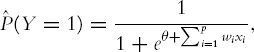
Relation to Linear and Logistic Regression Consider a neural network with a single output node and no hidden layers. For a dataset with p predictors, the output node receives x1, x2, . . ., xp, takes a weighted sum of these, and applies the g function. The output of the neural network is therefore
First, consider a numerical output variable y. If g is the identity function [g(s) = s], the output is simply

This is exactly equivalent to the formulation of a multiple linear regression! This means that a neural network with no hidden layers, a single output node, and an identity function g searches only for linear relationships between the response and the predictors.
Now consider a binary output variable y. If g is the logistic function, the output is simply
which is equivalent to the logistic regression formulation!
In both cases, although the formulation is equivalent to the linear and logistic regression models, the resulting estimates for the weights (coefficients in linear and logistic regression) can differ because the estimation method is different. The neural net estimation method is different from least squares, the method used to calculate coefficients in linear regression, or the maximum-likelihood method used in logistic regression. We explain below the method by which the neural network learns.
Neural networks perform best when the predictors and response variables are on a scale of [0,1]. For this reason, all variables should be scaled to a [0,1] interval before entering them into the network. For a numerical variable X that takes values in the range [a, b] (a < b), we normalize the measurements by subtracting a and dividing by b – a. The normalized measurement is then
Note that if [a, b] is within the [0,1] interval, the original scale will be stretched.
If a and b are not known, we can estimate them from the minimal and maximal values of X in the data. Even if new data exceed this range by a small amount, yielding normalized values slightly lower than 0 or larger than 1, this will not affect the results much.
For binary variables, no adjustment needs to be made other than creating dummy variables. For categorical variables with m categories, if they are ordinal in nature, a choice of m fractions in [0,1] should reflect their perceived ordering. For example, if four ordinal categories are equally distant from each other, we can map them to [0, 0.25, 0.5, 1]. If the categories are nominal, transforming into m-1 dummies is a good solution.
Another operation that improves the performance of the network is to transform highly skewed predictors. In business applications, there tend to be many highly right-skewed variables (such as income). Taking a log transform of a right-skewed variable will usually spread out the values more symmetrically.
Training the model means estimating the weights θj and wij that lead to the best predictive results. The process that we described earlier for computing the neural network output for an observation is repeated for all the observations in the training set. For each observation the model produces a prediction that is then compared with the actual response value. Their difference is the error for the output node. However, unlike least squares or maximum likelihood, where a global function of the errors (e.g., sum of squared errors) is used for estimating the coefficients, in neural networks the estimation process uses the errors iteratively to update the estimated weights.
In particular, the error for the output node is distributed across all the hidden nodes that led to it, so that each node is assigned "responsibility" for part of the error. Each of these node-specific errors is then used for updating the weights.
Back Propagation of Error The most popular method for using model errors to update weights ("learning") is an algorithm called back propagation. As the name implies, errors are computed from the last layer (the output layer) back to the hidden layers.
Let us denote by ŷk the output from output node k. The error associated with output node k is computed by
errk = ŷk(1 – ŷk)(yk – ŷk)
Notice that this is similar to the ordinary definition of an error (yk- yk) multiplied by a correction factor. The weights are then updated as follows:

where l is a learning rate or weight decay parameter, a constant ranging typically between 0 and 1, which controls the amount of change in weights from one iteration to the other.
In our example, the error associated with the output node for the first observation is (0.506)(1 −0.506)(1- 0.506) = 0.123. This error is then used to compute the errors associated with the hidden layer nodes, and those weights are updated accordingly using a formula similar to (11.2).
Two methods for updating the weights are case updating and batch updating. In case updating, the weights are updated after each observation is run through the network (called a trial). For example, if we used case updating in the tiny example, the weights would first be updated after running observation 1 as follows: Using a learning rate of 0.5, the weights θ6 and w3,6, w4,6, and w5,6 are updated to

These new weights are next updated after the second observation is run through the network, the third, and so on, until all observations are used. This is called one epoch, sweep, or iteration through the data. Typically, there are many epochs.
In batch updating, the entire training set is run through the network before each updating of weights takes place. In that case, the errors errk in the updating equation is the sum of the errors from all observations. In practice, case updating tends to yield more accurate results than batch updating but requires a longer runtime. This is a serious consideration since, even in batch updating, hundreds or even thousands of sweeps through the training data are executed.
When does the updating stop? The most common conditions are one of the following:
When the new weights are only incrementally different from those of the preceding iteration
When the misclassification rate reaches a required threshold
When the limit on the number of runs is reached
Let us examine the output from running a neural network on the tiny data. Following Figures 11.2 and 11.3, we used a single hidden layer with three nodes. The weights and classification matrix are shown in Figure 11.4. We can see that the network misclassifies all 1 observations and correctly classifies all 0 observations. This is not surprising since the number of observations is too small for estimating the 13 weights. However, for purposes of illustration we discuss the remainder of the output.

Figure 11.4. OUTPUT FOR NEURAL NETWORK WITH A SINGLE HIDDEN LAYER WITH THREE NODES FOR THE TINY DATA EXAMPLE
Note
To run a neural net in XLMiner, choose the Neural Network option in either the Prediction or Classification menu, depending on whether your response variable is quantitative or categorical. There are several options that the user can choose, which are described in the software guide. Notice, however, two points:
Normalize input data applies standard normalization (subtracting the mean and dividing by the standard deviation). Scaling to a [0,1] interval should be done beforehand.
XLMiner employs case updating. The user can specify the number of epochs to run.
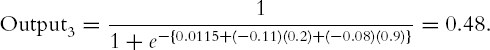
The final network weights are shown in two tables in the XLMiner output under Inter-layer connection weights. The upper table shows these weights in a format similar to that of our previous diagrams. The first table in Figure 11.4 shows the weights that connect the input layer and the hidden layer. The bias nodes in the last column are the weights θ3, θ4, and θ5. The weights in this table are used to compute the output of the hidden layer nodes. Figure 11.5 shows these weights in a format similar to that of our previous diagrams. The weights were computed iteratively after choosing a random initial set of weights (like the set we chose in Figure 11.3). We use the weights in the way we described earlier to compute the hidden layer's output. For instance, for the first observation, the output of our previous node 3 (denoted Node #1 in XLMiner) is
Similarly, we can compute the output from the two other hidden nodes for the same observation and get output4 = 046 and output5 = 0.51.
The second table in Figure 11.4 gives the weights connecting the hidden and output layer nodes. Note that XLMiner uses two output nodes even though we have a binary response. This is equivalent to using a single node with a cutoff value. To compute the output from the (first) output node for the first observation, we use the outputs from the hidden layer that we computed above, and get
This is the probability shown in the bottom-most table in Figure 11.4 (for observation 1), which gives the neural network's predicted probabilities and the classifications based on these values. The probabilities for the other five observations are computed equivalently, replacing the input value in the computation of the hidden layer outputs and then plugging these outputs into the computation for the output layer.
Let us apply the network training process to some real data: U.S. automobile accidents that have been classified by their level of severity as no injury, injury, or fatality. A firm might be interested in developing a system for quickly classifying the severity of an accident, based on initial reports and associated data in the system (some of which rely on GPS-assisted reporting). Such a system could be used to assign emergency response team priorities. Figure 11.6 shows a small extract (999 records, 4 predictor variables) from a U.S. government database. The explanation of the four predictor variables and response is given in Table 11.2.

Table 11.2. DESCRIPTION OF VARIABLES FOR AUTOMOBILE ACCIDENT EXAMPLE
ALCHL I | Presence (1) or absence (2) of alcohol |
PROFIL I R | Profile of the roadway: level (1), grade (2), hillcrest (3), other (4), unknown (5) |
SUR COND | Surface condition of the road: dry (1), wet (2), snow/slush (3), ice (4), sand/dirt (5), other (6), unknown (7) |
VEH INVL | Number of vehicles involved |
MAX SEV IR | Presence of injuries/fatalities: no injuries (0), injury (1), fatality (2) |
With the exception of alcohol involvement and a few other variables in the larger database, most of the variables are ones that we might reasonably expect to be available at the time of the initial accident report, before accident details and severity have been determined by first responders. A data mining model that could predict accident severity on the basis of these initial reports would have value in allocating first responder resources.
To use a neural net architecture for this classification problem we use four nodes in the input layer, one for each of the four predictors, and three neurons (one for each class) in the output layer. We use a single hidden layer and experiment with the number of nodes. Increasing the number of nodes from four to eight and examining the resulting confusion matrices, we find that five nodes gave a good balance between improving the predictive performance on the training set without deteriorating the performance on the validation set. In fact, networks with more than five nodes in the hidden layer performed as well as the five-node network.
Note that there is a total of five connections from each node in the input layer to each node in the hidden layer, a total of 4 × 5 = 20 connections between the input layer and the hidden layer. In addition, there is a total of three connections from each node in the hidden layer to each node in the output layer, a total of 5 × 3 = 15 connections between the hidden layer and the output layer.
We train the network on the training partition of 600 records. Each iteration in the neural network process consists of presentation to the input layer of the predictors in a case, followed by successive computations of the outputs of the hidden layer nodes and the output layer nodes using the appropriate weights. The output values of the output layer nodes are used to compute the error. This error is used to adjust the weights of all the connections in the network using the backward propagation algorithm to complete the iteration. Since the training data has 600 cases, one sweep through the data, termed an epoch, consists of 600 iterations. We will train the network using 30 epochs, so there will be a total of 18,000 iterations. The resulting classification results, error rates, and weights following the last epoch of training the neural net on this data are shown in Figure 11.7.
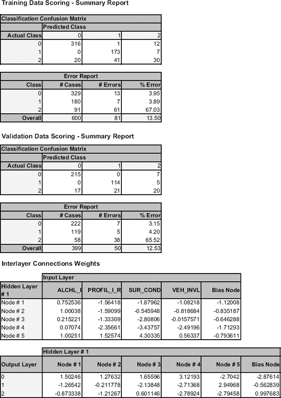
Figure 11.7. XLMINER OUTPUT FOR NEURAL NETWORK FOR ACCIDENT DATA, WITH FIVE NODES IN THE HIDDEN LAYER, AFTER 30 EPOCHS
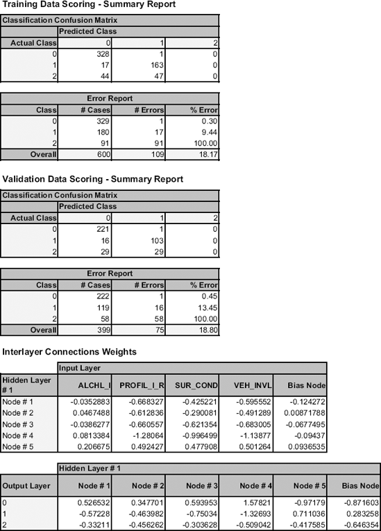
Note that had we stopped after only one pass of the data (600 iterations), the error would have been much worse, and none of the fatal accidents (coded as 2) would have been spotted, as can be seen in Figure 11.8. Our results can depend on how we set the different parameters, and there are a few pitfalls to avoid. We discuss these next.
A weakness of the neural network is that it can easily overfit the data, causing the error rate on validation data (and most important, on new data) to be too large. It is therefore important to limit the number of training epochs and not to overtrain the data. As in classification and regression trees, overfitting can be detected by examining the performance on the validation set and seeing when it starts deteriorating (while the training set performance is still improving). This approach is used in some algorithms (but not in XLMiner) to limit the number of training epochs: Periodically, the error rate on the validation dataset is computed while the network is being trained. The validation error decreases in the early epochs of the training, but after awhile it begins to increase. The point of minimum validation error is a good indicator of the best number of epochs for training, and the weights at that stage are likely to provide the best error rate in new data.

To illustrate the effect of overfitting, compare the confusion matrices of the 5-node network (Figure 11.7) with those from a 25-node network (Figure 11.9). Both networks perform similarly on the training set, but the 25-node network does worse on the validation set.
When the neural network is used for predicting a numerical response, the resulting output needs to be scaled back to the original units of that response. Recall that numerical variables (both predictor and response variables) are usually rescaled to a [0,1] interval before being used by the network. The output therefore will also be on a [0,1] scale. To transform the prediction back to the original y units, which were in the range [a, b], we multiply the network output by b – a and add a.
When the neural net is used for classification and we have m classes, we will obtain an output from each of the m output nodes. How do we translate these m outputs into a classification rule? Usually, the output node with the largest value determines the net's classification.
In the case of a binary response (m = 2), we can use just one output node with a cutoff value to map a numerical output value to one of the two classes. Although we typically use a cutoff of 0.5 with other classifiers, in neural networks there is a tendency for values to cluster around 0.5 (from above and below). An alternative is to use the validation set to determine a cutoff that produces reasonable predictive performance.
One of the time-consuming and complex aspects of training a model using back propagation is that we first need to decide on a network architecture. This means specifying the number of hidden layers and the number of nodes in each layer. The usual procedure is to make intelligent guesses using past experience and to do several trial-and-error runs on different architectures. Algorithms exist that grow the number of nodes selectively during training or trim them in a manner analogous to what is done in classification and regression trees (see Chapter 9). Research continues on such methods. As of now, no automatic method seems clearly superior to the trial-and-error approach. A few general guidelines for choosing an architecture follow.
Number of Hidden Layers The most popular choice for the number of hidden layers is one. A single hidden layer is usually sufficient to capture even very complex relationships between the predictors.
Size of Hidden Layer The number of nodes in the hidden layer also determines the level of complexity of the relationship between the predictors that the network captures. The trade-off is between under- and overfitting. Using too few nodes might not be sufficient to capture complex relationships (recall the special cases of a linear relationship such as in linear and logistic regression, in the extreme case of zero nodes or no hidden layer). On the other hand, too many nodes might lead to overfitting. A rule of thumb is to start with p (number of predictors) nodes and gradually decrease or increase a bit while checking for overfitting.
Number of Output Nodes For a binary response, a single node is sufficient, and a cutoff is used for classification. For a categorical response with m >2 classes, the number of nodes should equal the number of classes. Finally, for a numerical response, typically a single output node is used unless we are interested in predicting more than one function.
In addition to the choice of architecture, the user should pay attention to the choice of predictors. Since neural networks are highly dependent on the quality of their input, the choice of predictors should be done carefully, using domain knowledge, variable selection, and dimension reduction techniques before using the network. We return to this point in the discussion of advantages and weaknesses below.
Other parameters that the user can control are the learning rate (a.k.a. weight decay), l, and the momentum. The first is used primarily to avoid overfitting, by down-weighting new information. This helps to tone down the effect of outliers on the weights and avoids getting stuck in local optima. This parameter typically takes a value in the range [0, 1]. Berry and Linoff (2000) suggest starting with a large value (moving away from the random initial weights, thereby "learning quickly" from the data) and then slowly decreasing it as the iterations progress and the weights are more reliable. Han and Kamber (2001) suggest the more concrete rule of thumb of setting l = 1/(current number of iterations). This means that at the start, l = 1, during the second iteration it is l = 0.5, and then it keeps decaying toward l = 0. Notice that in XLMiner the default is l = 0, which means that the weights do not decay at all.
The second parameter, called momentum, is used to "keep the ball rolling" (hence the term momentum) in the convergence of the weights to the optimum. The idea is to keep the weights changing in the same direction as they did in the preceding iteration. This helps to avoid getting stuck in a local optimum. High values of momentum mean that the network will be "reluctant" to learn from data that want to change the direction of the weights, especially when we consider case updating. In general, values in the range 0–2 are used.
Neural networks are known to be "black boxes" in the sense that their output does not shed light on the patterns in the data that it models (like our brains). In fact, that is one of the biggest criticism of the method. However, in some cases it is possible to learn more about the relationships that the network captures, by conducting a sensitivity analysis on validation set. This is done by setting all predictor values to their mean and obtaining the network's prediction. Then the process is repeated by setting each predictor sequentially to its minimum (and then maximum) value. By comparing the predictions from different levels of the predictors, we can get a sense of which predictors affect predictions more and in what way.
As mentioned in Section 11.1, the most prominent advantage of neural networks is their good predictive performance. They are known to have high tolerance to noisy data and the ability to capture highly complicated relationships between the predictors and a response. Their weakest point is in providing insight into the structure of the relationship, hence their black-box reputation.
Several considerations and dangers should be kept in mind when using neural networks. First, although they are capable of generalizing from a set of examples, extrapolation is still a serious danger. If the network sees only cases in a certain range, its predictions outside this range can be completely invalid.
Second, neural networks do not have a built-in variable selection mechanism. This means that there is need for careful consideration of predictors. Combination with classification and regression trees (see Chapter 9) and other dimension reduction techniques (e.g., principal components analysis in Chapter 4) is often used to identify key predictors.
Third, the extreme flexibility of the neural network relies heavily on having sufficient data for training purposes. As our tiny example shows, a neural network performs poorly when the training set size is insufficient, even when the relationship between the response and predictors is very simple. A related issue is that in classification problems, the network requires sufficient records of the minority class in order to learn it. This is achieved by oversampling, as explained in Chapter 2.
Fourth, a technical problem is the risk of obtaining weights that lead to a local optimum rather than the global optimum, in the sense that the weights converge to values that do not provide the best fit to the training data. We described several parameters that are used to try to avoid this situation (such as controlling the learning rate and slowly reducing the momentum). However, there is no guarantee that the resulting weights are indeed the optimal ones.
Finally, a practical consideration that can determine the usefulness of a neural network is the timeliness of computation. Neural networks are relatively heavy on computation time, requiring a longer runtime than other classifiers. This runtime grows greatly when the number of predictors is increased (as there will be many more weights to compute). In applications where real-time or near-real-time prediction is required, runtime should be measured to make sure that it does not cause unacceptable delay in the decision making.
Credit Card Use. Consider the following hypothetical bank data on consumers' use of credit card credit facilities in Table 11.3. Create a small worksheet in Excel, like that used in Example 1, to illustrate one pass through a simple neural network.
11.1 Neural Net Evolution. A neural net typically starts out with random coefficients; hence, it produces essentially random predictions when presented with its first case. What is the key ingredient by which the net evolves to produce a more accurate prediction?
11.2 Neural Net Evolution. A neural net typically starts out with random coefficients; hence, it produces essentially random predictions when presented with its first case. What is the key ingredient by which the net evolves to produce a more accurate prediction?
11.3 Car Sales. Consider again the data on used cars (ToyotaCorolla.xls) with 1436 records and details on 38 attributes, including Price, Age, KM, HP, and other specifications. The goal is to predict the price of a used Toyota Corolla based on its specifications.
Use XLMiner's neural network routine to fit a model using the XLMiner default values for the neural net parameters, except normalizing the data. Record the RMS error for the training data and the validation data. Repeat the process, changing the number of epochs (and only this) to 300, 3000, and 10,000.
What happens to the RMS error for the training data as the number of epochs increases?
What happens to the RMS error for the validation data?
Comment on the appropriate number of epochs for the model.
Conduct a similar experiment to assess the effect of changing the number of layers in the network as well as the gradient descent step size.
11.4 Direct Mailing to Airline Customers. East-West Airlines has entered into a partnership with the wireless phone company Telcon to sell the latter's service via direct mail. The file EastWestAirlinesNN.xls contains a subset of a data sample of who has already received a test offer. About 13% accepted.
You are asked to develop a model to classify East-West customers as to whether they purchased a wireless phone service contract (target variable Phone Sale), a model that can be used to predict classifications for additional customers.
Using XLMiner, run a neural net model on these data, using the option to normalize the data, setting the number of epochs at 3000, and requesting lift charts for both the training and validation data. Interpret the meaning (in business terms) of the leftmost bar of the validation lift chart (the bar chart).
Table 11.3. DATA FOR CREDIT CARD EXAMPLE AND VARIABLE DESCRIPTIONSa
Years
Salary
Used Credit
Years = Number of years that a customer has been with the bank; Salary = customer's salary (in thousands of dollars); Used Credit 1 = customer has left an unpaid credit card balance at the end of at least one month in the prior year and 0 = balance was paid off at the end of each month.
4
43
0
18
65
1
1
53
0
3
95
0
15
88
1
6
112
1
Comment on the difference between the training and validation lift charts.
Run a second neural net model on the data, this time setting the number of epochs at 100. Comment now on the difference between this model and the model you ran earlier, and how overfitting might have affected results.
What sort of information, if any, is provided about the effects of the various variables?