
This chapter describes a flexible data-driven method that can be used for both classification (called classification tree) and prediction (called regression tree). Among the data-driven methods, trees are the most transparent and easy to interpret. Trees are based on separating observations into subgroups by creating splits on predictors. These splits create logical rules that are transparent and easily understandable, for examples "If Age<55 AND Education>12 THEN class=1." The resulting subgroups should be more homogeneous in terms of the outcome variable, thereby creating useful prediction or classification rules. We discuss the two key ideas underlying trees: recursive partitioning (for constructing the tree) and pruning (for cutting the tree back). In the context of tree construction, we also describe a few metrics of homogeneity that are popular in tree algorithms, for determining the homogeneity of the resulting subgroups of observations. We explain that pruning is a useful strategy for avoiding overfitting and show how it is done. We also describe alternative strategies for avoiding overfitting. As with other data-driven methods, trees require large amounts of data. However, once constructed, they are computationally cheap to deploy even on large samples. They also have other advantages such as being highly automated, robust to outliers, and can handle missing values. Finally, we describe how trees can be used for dimension reduction.
If one had to choose a classification technique that performs well across a wide range of situations without requiring much effort from the analyst while being readily understandable by the consumer of the analysis, a strong contender would be the tree methodology developed by Breiman et al. (1984). We discuss this classification procedure first; then in later sections we show how the procedure can be extended to prediction of a numerical outcome. The program that Breiman et al. created to implement these procedures was called CART (classification and regression trees). A related procedure is called C4.5.

Figure 9.1. BEST PRUNED TREE OBTAINED BY FITTING A FULL TREE TO THE TRAINING DATA AND PRUNING IT USING THE VALIDATION DATA
What is a classification tree? Figure 9.1 describes a tree for classifying bank customers who receive a loan offer as either acceptors or nonacceptors, as a function of information such as their income, education level, and average credit card expenditure. One of the reasons that tree classifiers are very popular is that they provide easily understandable classification rules (at least if the trees are not too large). Consider the tree in the example. The square terminal nodes are marked with 0 or 1 corresponding to a nonacceptor (0) or acceptor (1). The values in the circle nodes give the splitting value on a predictor. This tree can easily be translated into a set of rules for classifying a bank customer. For example, the middle left square node in this tree gives us the following rule:
In the following we show how trees are constructed and evaluated.
There are two key ideas underlying classification trees. The first is the idea of recursive partitioning of the space of the predictor variables. The second is the idea of pruning using validation data. In the next few sections we describe recursive partitioning and in subsequent sections explain the pruning methodology.
Let us denote the dependent (response) variable by y and the predictor variables by x1, x2, x3, ... , xp. In classification, the outcome variable will be a categorical variable. Recursive partitioning divides up the p-dimensional space of the x variables into nonoverlapping multidimensional rectangles. The X variables here are considered to be continuous, binary, or ordinal. This division is accomplished recursively (i.e., operating on the results of prior divisions). First, one of the variables is selected, say xi, and a value of xi, say si, is chosen to split the p-dimensional space into two parts: one part that contains all the points with xi si and the other with all the points with xi > si. Then one of these two parts is divided in a similar manner by choosing a variable again (it could be xi or another variable) and a split value for the variable. This results in three (multidimensional) rectangular regions. This process is continued so that we get smaller and smaller rectangular regions. The idea is to divide the entire x space up into rectangles such that each rectangle is as homogeneous or "pure" as possible. By pure we mean containing points that belong to just one class. (Of course, this is not always possible, as there may be points that belong to different classes but have exactly the same values for every one of the predictor variables.)
Let us illustrate recursive partitioning with an example.
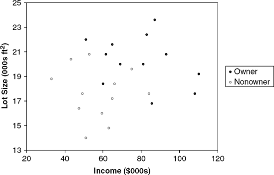
We again use the riding-mower example presented in Chapter 7. A riding-mower manufacturer would like to find a way of classifying families in a city into those likely to purchase a riding mower and those not likely to buy one. A pilot random sample of 12 owners and 12 nonowners in the city is undertaken. The data are shown and plotted in Table 9.1 and Figure 9.2.
If we apply the classification tree procedure to these data, the procedure will choose Lot Size for the first split with a splitting value of 19. The (x1, x2) space is now divided into two rectangles, one with Lot Size≤ 19 and the other with Lot Size> 19. This is illustrated in Figure 9.3.
Notice how the split has created two rectangles, each of which is much more homogeneous than the rectangle before the split. The upper rectangle contains points that are mostly owners (nine owners and three nonowners) and the lower rectangle contains mostly nonowners (nine nonowners and three owners).
Table 9.1. LOT SIZE, INCOME, AND OWNERSHIP OF A RIDING MOWER FOR 24 HOUSEHOLDS
Household Number | Income ($000s) | Lot Size (000s ft2) | Ownership of Riding Mower |
|---|---|---|---|
1 | 60 | 18.4 | Owner |
2 | 85.5 | 16.8 | Owner |
3 | 64.8 | 21.6 | Owner |
4 | 61.5 | 20.8 | Owner |
5 | 87 | 23.6 | Owner |
6 | 110.1 | 19.2 | Owner |
7 | 108 | 17.6 | Owner |
8 | 82.8 | 22.4 | Owner |
9 | 69 | 20 | Owner |
10 | 93 | 20.8 | 20.8 |
11 | 51 | 22 | Owner |
12 | 81 | 20 | Owner |
13 | 75 | 19.6 | Nonowner |
14 | 52.8 | 20.8 | Nonowner |
15 | 64.8 | 17.2 | Nonowner |
16 | 43.2 | 20.4 | Nonowner |
17 | 84 | 17.6 | Nonowner |
18 | 49.2 | 17.6 | Nonowner |
19 | 59.4 | 16 | Nonowner |
20 | 66 | 18.4 | Nonowner |
21 | 47.4 | 16.4 | Nonowner |
22 | 33 | 18.8 | Nonowner |
23 | 51 | 14 | Nonowner |
24 | 63 | 14.8 |

How was this particular split selected? The algorithm examined each variable (in this case, Income and Lot Size) and all possible split values for each variable to find the best split. What are the possible split values for a variable? They are simply the midpoints between pairs of consecutive values for the variable. The possible split points for Income are {38.1, 45.3, 50.1, ..., 109.5} and those for Lot Size are {14.4, 15.4, 16.2, ..., 23}. These split points are ranked according to how much they reduce impurity (heterogeneity) in the resulting rectangle. A pure rectangle is one that is composed of a single class (e.g., owners). The reduction in impurity is defined as overall impurity before the split minus the sum of the impurities for the two rectangles that result from a split.
Categorical Predictors The above description used numerical predictors. However, categorical predictors can also be used in the recursive partitioning context. To handle categorical predictors, the split choices for a categorical predictor are all ways in which the set of categories can be divided into two subsets. For example, a categorical variable with four categories, say {a,b,c,d}, can be split in seven ways into two subsets: {a} and {b,c,d}; {b} and {a,c,d}; {c} and {a,b,d}; {d} and {a,b,c}; {a,b} and {c,d}; {a,c} and {b,d}; and {a,d} and {b,c}. When the number of categories is large, the number of splits becomes very large. XLMiner supports only binary categorical variables (coded as numbers). If you have a categorical predictor that takes more than two values, you will need to replace the variable with several dummy variables, each of which is binary in a manner that is identical to the use of dummy variables in regression.[17]

There are a number of ways to measure impurity. The two most popular measures are the Gini index and an entropy measure. We describe both next. Denote the m classes of the response variable by k = 1, 2, ..., m.
The Gini impurity index for a rectangle A is defined by
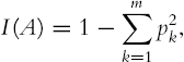
where pk is the proportion of observations in rectangle A that belong to class k. This measure takes values between 0 (if all the observations belong to the same class) and (m − 1)/m (when all m classes are equally represented). Figure 9.4 shows the values of the Gini index for a two-class case as a function ofpk. It can be seen that the impurity measure is at its peak when pk = 0.5 (i.e., when the rectangle contains 50% of each of the two classes).[18]
A second impurity measure is the entropy measure. The entropy for a rectangle A is defined by
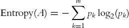
[to compute log2(x) in Excel, use the function = log(x, 2)]. This measure ranges between 0 (most pure, all observations belong to the same class) and log2(m) (when all m classes are represented equally). In the two-class case, the entropy measure is maximized (like the Gini index) at pk = 0.5.
Let us compute the impurity in the riding-mower example before and after the first split (using Lot Size with the value of 19). The unsplit dataset contains 12 owners and 12 nonowners. This is a two-class case with an equal number of observations from each class. Both impurity measures are therefore at their maximum value: Gini = 0.5 and entropy = log2(2) = 1. After the split, the upper rectangle contains nine owners and three nonowners. The impurity measures for this rectangle are Gini = 1 − 0.25 − 0.75 = 0.375 and entropy = −0.25 log2(0.25) − 0.75 log2(0.75) = 0.811. The lower rectangle contains three owners and nine nonowners. Since both impurity measures are symmetric, they obtain the same values as for the upper rectangle.
The combined impurity of the two rectangles that were created by the split is a weighted average of the two impurity measures, weighted by the number of observations in each (in this case we ended up with 12 observations in each rectangle, but in general the number of observations need not be equal): Gini = (12/24)(0.375) + (12/24)(0.375) = 0.375 and entropy = (12/24)(0.811) + (12/24)(0.811) = 0.811. Thus, the Gini impurity index decreased from 0.5 before the split to 0.375 after the split. Similarly, the entropy impurity measure decreased from 1 before the split to 0.811 after the split.
By comparing the reduction in impurity across all possible splits in all possible predictors, the next split is chosen. If we continue splitting the mower data, the next split is on the Income variable at the value 84.75. Figure 9.5 shows that once again the tree procedure has astutely chosen to split a rectangle to increase the purity of the resulting rectangles. The left lower rectangle, which contains data points with Income ≤ 84.75 and Lot Size ≤ 19, has all points that are nonowners (with one exception); whereas the right lower rectangle, which contains data points with Income > 84.75 and Lot Size ≤ 19, consists exclusively of owners. We can see how the recursive partitioning is refining the set of constituent rectangles to become purer as the algorithm proceeds. The final stage of the recursive partitioning is shown in Figure 9.6.

Figure 9.5. SPLITTING THE 24 OBSERVATIONS BY LOT SIZE VALUE OF $19K, AND THEN INCOME VALUE OF $84.75K

Figure 9.6. FINAL STAGE OF RECURSIVE PARTITIONING; EACH RECTANGLE CONSISTING OF A SINGLE CLASS (OWNERS OR NONOWNERS)
Notice that each rectangle is now pure: It contains data points from just one of the two classes.
The reason the method is called a classification tree algorithm is that each split can be depicted as a split of a node into two successor nodes. The first split is shown as a branching of the root node of a tree in Figure 9.7. The tree representing the first three splits is shown in Figure 9.8. The full-grown tree is shown in Figure 9.9.
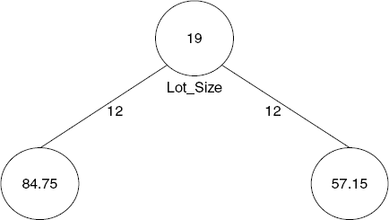

We represent the nodes that have successors by circles. The numbers inside the circles are the splitting values and the name of the variable chosen for splitting at that node is shown below the node. The numbers on the left fork at a decision node are the number of records in the decision node that had values less than or equal to the splitting value, and the numbers on the right fork show the number that had a greater value. These are called decision nodes because if we were to use a tree to classify a new observation for which we knew only the values of the predictor variables, we would "drop" the observation down the tree in such a way that at each decision node the appropriate branch is taken until we get to a node that has no successors. Such terminal nodes are called the leaves of the tree. Each leaf node is depicted with a rectangle rather than a circle, and corresponds to one of the final rectangles into which the x space is partitioned.
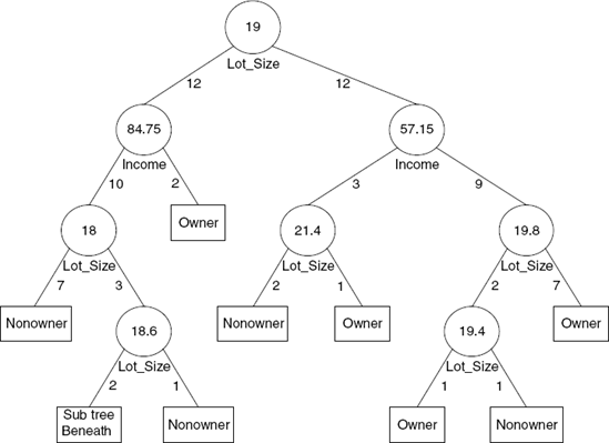
To classify a new observation, it is "dropped" down the tree. When it has dropped all the way down to a terminal leaf, we can assign its class simply by taking a "vote" of all the training data that belonged to the leaf when the tree was grown. The class with the highest vote is assigned to the new observation. For instance, a new observation reaching the rightmost leaf node in Figure 9.9, which has a majority of observations that belong to the owner class, would be classified as "owner." Alternatively, if a single class is of interest, the algorithm counts the number of "votes" for this class, converts it to a proportion (estimated probability), then compares it to a user-specified cutoff value. See Chapter 5 for further discussion of the use of a cutoff value in classification, for cases where a single class is of interest.
In a binary classification situation (typically, with a success class that is relatively rare and of particular interest), we can also establish a lower cutoff to better capture those rare successes (at the cost of lumping in more nonsuccesses as successes). With a lower cutoff, the votes for the success class only need attain that lower cutoff level for the entire leaf to be classified as a success. The cutoff therefore determines the proportion of votes needed for determining the leaf class. It is useful to note that the type of trees grown by CART (called binary trees) have the property that the number of leaf nodes is exactly one more than the number of decision nodes.
To assess the accuracy of a tree in classifying new cases, we use the tools and criteria that were discussed in Chapter 5. We start by partitioning the data into training and validation sets. The training set is used to grow the tree, and the validation set is used to assess its performance. In the next section we discuss an important step in constructing trees that involves using the validation data. In that case, a third set of test data is preferable for assessing the accuracy of the final tree.
Each observation in the validation (or test) data is dropped down the tree and classified according to the leaf node it reaches. These predicted classes can then be compared to the actual memberships via a classification matrix. When a particular class is of interest, a lift chart is useful for assessing the model's ability to capture those members. We use the following example to illustrate this.
Universal Bank is a relatively young bank that is growing rapidly in terms of overall customer acquisition. The majority of these customers are liability customers with varying sizes of relationship with the bank. The customer base of asset customers is quite small, and the bank is interested in growing this base rapidly to bring in more loan business. In particular, it wants to explore ways of converting its liability customers to personal loan customers.
A campaign the bank ran for liability customers showed a healthy conversion rate of over 9% successes. This has encouraged the retail marketing department to devise smarter campaigns with better target marketing. The goal of our analysis is to model the previous campaign's customer behavior to analyze what combination of factors make a customer more likely to accept a personal loan. This will serve as the basis for the design of a new campaign.
The bank's dataset includes data on 5000 customers. The data include customer demographic information (age, income, etc.), customer response to the last personal loan campaign (Personal Loan), and the customer's relationship with the bank (mortgage, securities account, etc.). Among these 5000 customers, only 480 (= 9.6%) accepted the personal loan that was offered to them in the earlier campaign. Table 9.2 contains a sample of the bank's customer database for 20 customers, to illustrate the structure of the data.
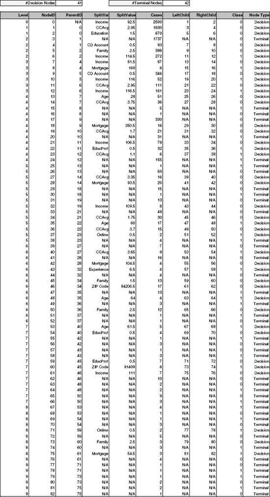
After randomly partitioning the data into training (2500 observations), validation (1500 observations), and test (1000 observations) sets, we use the training data to construct a full-grown tree. The first four levels of the tree are shown in Figure 9.10, and the complete results are given in a form of a table in Figure 9.11.
Even with just four levels, it is difficult to see the complete picture. A look at the top tree node or the first row of the table reveals that the first predictor that is chosen to split the data is Income, with a value of 92.5 ($000s).
Since the full-grown tree leads to completely pure terminal leaves, it is 100% accurate in classifying the training data. This can be seen in Figure 9.12. In contrast, the classification matrix for the validation and test data (which were not used to construct the full-grown tree) show lower classification accuracy. The main reason is that the full-grown tree overfits the training data (to complete accuracy!). This motivates the next section, where we describe ways to avoid overfitting by either stopping the growth of the tree before it is fully grown or by pruning the full-grown tree.
Table 9.2. SAMPLE OF DATA FOR 20 CUSTOMERS OF UNIVERSAL BANK
ID | Age | Professional Experience | Income | Family Size | CC Avg | Education | Mortgage | Personal Loan | Securities Account | CD Account | Online Banking | Credit Card |
|---|---|---|---|---|---|---|---|---|---|---|---|---|
1 | 25 | 1 | 49 | 4 | 1.60 | UG | 0 | No | Yes | No | No | No |
2 | 45 | 19 | 34 | 3 | 1.50 | UG | 0 | No | Yes | No | No | No |
3 | 39 | 15 | 11 | 1 | 1.00 | UG | 0 | No | No | No | No | No |
4 | 35 | 9 | 100 | 1 | 2.70 | Grad | 0 | No | No | No | No | No |
5 | 35 | 8 | 45 | 4 | 1.00 | Grad | 0 | No | No | No | No | Yes |
6 | 37 | 13 | 29 | 4 | 0.40 | Grad | 155 | No | No | No | Yes | No |
7 | 53 | 27 | 72 | 2 | 1.50 | Grad | 0 | No | No | No | Yes | No |
8 | 50 | 24 | 22 | 1 | 0.30 | Prof | 0 | No | No | No | No | Yes |
9 | 35 | 10 | 81 | 3 | 0.60 | Grad | 104 | No | No | No | Yes | No |
10 | 34 | 9 | 180 | 1 | 8.90 | Prof | 0 | Yes | No | No | No | No |
11 | 65 | 39 | 105 | 4 | 2.40 | Prof | 0 | No | No | No | No | No |
12 | 29 | 5 | 45 | 3 | 0.10 | Grad | 0 | No | No | No | Yes | No |
13 | 48 | 23 | 114 | 2 | 3.80 | Prof | 0 | No | Yes | No | No | No |
14 | 59 | 32 | 40 | 4 | 2.50 | Grad | 0 | No | No | No | Yes | No |
15 | 67 | 41 | 112 | 1 | 2.00 | UG | 0 | No | Yes | No | No | No |
16 | 60 | 30 | 22 | 1 | 1.50 | Prof | 0 | No | No | No | Yes | Yes |
17 | 38 | 14 | 130 | 4 | 4.70 | Prof | 134 | Yes | No | No | No | No |
18 | 42 | 18 | 81 | 4 | 2.40 | UG | 0 | No | No | No | No | No |
19 | 46 | 21 | 193 | 2 | 8.10 | Prof | 0 | Yes | No | No | No | No |
20 | 55 | 28 | 21 | 1 | 0.50 | Grad | 0 | No | Yes | No | No | Yes |


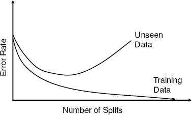
As the last example illustrated, using a full-grown tree (based on the training data) leads to complete overfitting of the data. As discussed in Chapter 5, overfitting will lead to poor performance on new data. If we look at the overall error at the various levels of the tree, it is expected to decrease as the number of levels grows until the point of overfitting. Of course, for the training data the overall error decreases more and more until it is zero at the maximum level of the tree. However, for new data, the overall error is expected to decrease until the point where the tree models the relationship between class and the predictors. After that, the tree starts to model the noise in the training set, and we expect the overall error for the validation set to start increasing. This is depicted in Figure 9.13. One intuitive reason for the overfitting at the high levels of the tree is that these splits are based on very small numbers of observations. In such cases, class difference is likely to be attributed to noise rather than predictor information.
Two ways to try and avoid exceeding this level, thereby limiting overfitting, are by setting rules to stop tree growth or, alternatively, by pruning the full-grown tree back to a level where it does not overfit. These solutions are discussed below.
One can think of different criteria for stopping the tree growth before it starts overfitting the data. Examples are tree depth (i.e., number of splits), minimum number of observations in a node, and minimum reduction in impurity. The problem is that it is not simple to determine what is a good stopping point using such rules.
Previous methods developed were based on the idea of recursive partitioning, using rules to prevent the tree from growing excessively and overfitting the training data. One popular method called CHAID (chi-squared automatic interaction detection) is a recursive partitioning method that predates classification and regression tree (CART) procedures by several years and is widely used in database marketing applications to this day. It uses a well-known statistical test (the chi-square test for independence) to assess whether splitting a node improves the purity by a statistically significant amount. In particular, at each node we split on the predictor that has the strongest association with the response variable. The strength of association is measured by the p-value of a chi-squared test of independence. If for the best predictor the test does not show a significant improvement, the split is not carried out, and the tree is terminated. This method is more suitable for categorical predictors, but it can be adapted to continuous predictors by binning the continuous values into categorical bins.
An alternative solution that has proven to be more successful than stopping tree growth is pruning the full-grown tree. This is the basis of methods such as CART [developed by Breiman et al. (1984), implemented in multiple data mining software packages such as SAS Enterprise Miner, CART, MARS, and in XLMiner] and C4.5 implemented in packages such as IBM Modeler (previously Clementine by SPSS). In C4.5 the training data are used both for growing and pruning the tree. In CART the innovation is to use the validation data to prune back the tree that is grown from training data. CART and CART-like procedures use validation data to prune back the tree that has deliberately been overgrown using the training data. This approach is also used by XLMiner.
The idea behind pruning is to recognize that a very large tree is likely to be overfitting the training data and that the weakest branches, which hardly reduce the error rate, should be removed. In the mower example the last few splits resulted in rectangles with very few points (indeed, four rectangles in the full tree had just one point). We can see intuitively that these last splits are likely simply to be capturing noise in the training set rather than reflecting patterns that would occur in future data, such as the validation data. Pruning consists of successively selecting a decision node and redesignating it as a leaf node [lopping off the branches extending beyond that decision node (its subtree) and thereby reducing the size of the tree]. The pruning process trades off misclassification error in the validation dataset against the number of decision nodes in the pruned tree to arrive at a tree that captures the patterns but not the noise in the training data. Returning to Figure 9.13, we would like to find the point where the curve for the unseen data begins to increase.
To find this point, the CART algorithm uses a criterion called the cost complexity of a tree to generate a sequence of trees that are successively smaller to the point of having a tree with just the root node. (What is the classification rule for a tree with just one node?). This means that the first step is to find the best subtree of each size (1, 2, 3, ...). Then, to chose among these, we want the tree that minimizes the error rate of the validation set. We then pick as our best tree the one tree in the sequence that gives the smallest misclassification error in the validation data.
Constructing the best tree of each size is based on the cost complexity (CC) criterion, which is equal to the misclassification error of a tree (based on the training data) plus a penalty factor for the size of the tree. For a tree T that has L(T) leaf nodes, the cost complexity can be written as
where err(T) is the fraction of training data observations that are misclassified by tree T and is a penalty factor for tree size. When α = 0, there is no penalty for having too many nodes in a tree, and the best tree using the cost complexity criterion is the full-grown unpruned tree. When we increase to a very large value, the penalty cost component swamps the misclassification error component of the cost complexity criterion function, and the best tree is simply the tree with the fewest leaves: namely, the tree with simply one node. The idea is therefore to start with the full-grown tree and then increase the penalty factor gradually until the cost complexity of the full tree exceeds that of a subtree. Then the same procedure is repeated using the subtree. Continuing in this manner, we generate a succession of trees with a diminishing number of nodes all the way to a trivial tree consisting of just one node.
From this sequence of trees it seems natural to pick the one that gave the minimum misclassification error on the validation dataset. We call this the minimum error tree. To illustrate this, Figure 9.14 shows the error rate for both the training and validation data as a function of the tree size. It can be seen that the training set error steadily decreases as the tree grows, with a noticeable drop in error rate between two and three nodes. The validation set error rate, however, reaches a minimum at 11 nodes and then starts to increase as the tree grows. At this point the tree is pruned and we obtain the minimum error tree.
A further enhancement is to incorporate the sampling error, which might cause this minimum to vary if we had a different sample. The enhancement uses the estimated standard error of the error rate to prune the tree even further (to the validation error rate, which is one standard error above the minimum.) In other words, the "best pruned tree" is the smallest tree in the pruning sequence that has an error within one standard error of the minimum error tree. The best pruned tree for the loan acceptance example is shown in Figure 9.15.
Returning to the loan acceptance example, we expect that the classification accuracy of the validation set using the pruned tree would be higher than using the full-grown tree (compare Figure 9.12 with Figure 9.16). However, the performance of the pruned tree on the validation data is not fully reflective of the performance on completely new data because the validation data were actually used for the pruning. This is a situation where it is particularly useful to evaluate the performance of the chosen model, whatever it may be, on a third set of data, the test set, which has not been used at all. In our example, the pruned tree applied to the test data yields an overall error rate of 1.7% (compared to 0% for the training data and 1.6% for the validation data). Although in this example the performance on the validation and test sets is similar, the difference can be larger for other datasets.

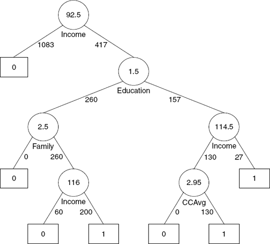
As described in Section 9.1, classification trees provide easily understandable classification rules (if the trees are not too large). Each leaf is equivalent to a classification rule. Returning to the example, the middle left leaf in the best pruned tree gives us the rule
However, in many cases the number of rules can be reduced by removing redundancies. For example, the rule
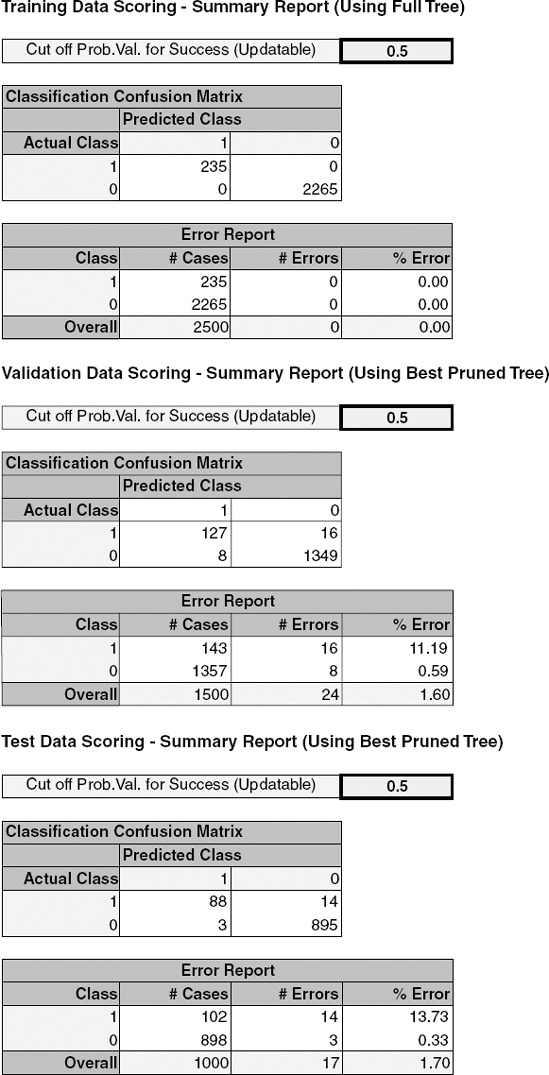
Figure 9.16. CLASSIFICATION MATRIX AND ERROR RATES FOR THE TRAINING, VALIDATION, AND TEST DATA BASED ON THE PRUNED TREE
IF(Income > 114.5) AND (Education > 1.5) THEN Class = 1.
This transparency in the process and understandability of the algorithm that leads to classifying an observation as belonging to a certain class is very advantageous in settings where the final classification is not solely of interest. Berry and Linoff (2000) give the example of health insurance underwriting, where the insurer is required to show that coverage denial is not based on discrimination. By showing rules that led to denial (e.g., income < $20K AND low credit history), the company can avoid lawsuits. Compared to the output of other classifiers, such as discriminant functions, tree-based classification rules are easily explained to managers and operating staff. Their logic is certainly far more transparent than that of weights in neural networks!
Classification trees can be used with an outcome that has more than two classes. In terms of measuring impurity, the two measures that were presented earlier (the Gini impurity index and the entropy measure) were defined for m classes and hence can be used for any number of classes. The tree itself would have the same structure, except that its terminal nodes would take one of the m-class labels.
The tree method can also be used for numerical response variables. Regression trees for prediction operate in much the same fashion as classification trees. The output variable, Y, is a numerical variable in this case, but both the principle and the procedure are the same: Many splits are attempted, and for each, we measure "impurity" in each branch of the resulting tree. The tree procedure then selects the split that minimizes the sum of such measures. To illustrate a regression tree, consider the example of predicting prices of Toyota Corolla automobiles (from Chapter 6). The dataset includes information on 1000 sold Toyota Corolla cars (we use the first 1000 cars from the dataset ToyotoCorolla.xls). The goal is to find a predictive model of price as a function of 10 predictors (including mileage, horsepower, number of doors, etc.). A regression tree for these data was built using a training set of 600. The best pruned tree is shown in Figure 9.17.

It can be seen that only two predictors show up as useful for predicting price: the age of the car and its horsepower. There are three details that are different in regression trees than in classification trees: prediction, impurity measures, and evaluating performance. We describe these next.
Predicting the value of the response Y for an observation is performed in a fashion similar to the classification case: The predictor information is used for "dropping" down the tree until reaching a leaf node. For instance, to predict the price of a Toyota Corolla with Age = 55 and Horsepower = 86, we drop it down the tree and reach the node that has the value $8842.65. This is the price prediction for this car according to the tree. In classification trees the value of the leaf node (which is one of the categories) is determined by the "voting" of the training data that were in that leaf. In regression trees the value of the leaf node is determined by the average of the training data in that leaf. In the example above, the value $8842.6 is the average of the 56 cars in the training set that fall in the category of Age > 52.5 AND Horsepower < 93.5.
We described two types of impurity measures for nodes in classification trees: the Gini index and the entropy-based measure. In both cases the index is a function of the ratio between the categories of the observations in that node. In regression trees a typical impurity measure is the sum of the squared deviations from the mean of the leaf. This is equivalent to the squared errors because the mean of the leaf is exactly the prediction. In the example above, the impurity of the node with the value $8842.6 is computed by subtracting $8842.6 from the price of each of the 56 cars in the training set that fell in that leaf, then squaring these deviations and summing them up. The lowest impurity possible is zero, when all values in the node are equal.
As stated above, predictions are obtained by averaging the values of the responses in the nodes. We therefore have the usual definition of predictions and errors. The predictive performance of regression trees can be measured in the same way that other predictive methods are evaluated, using summary measures such as RMSE and charts such as lift charts.
Tree methods are good off-the-shelf classifiers and predictors. They are also useful for variable selection, with the most important predictors usually showing up at the top of the tree. Trees require relatively little effort from users in the following senses: First, there is no need for transformation of variables (any monotone transformation of the variables will give the same trees). Second, variable subset selection is automatic since it is part of the split selection. In the loan example notice that the best pruned tree has automatically selected just four variables (Income, Education, Family, and CCAvg) out of the set 14 variables available.
Trees are also intrinsically robust to outliers since the choice of a split depends on the ordering of observation values and not on the absolute magnitudes of these values. However, they are sensitive to changes in the data, and even a slight change can cause very different splits!
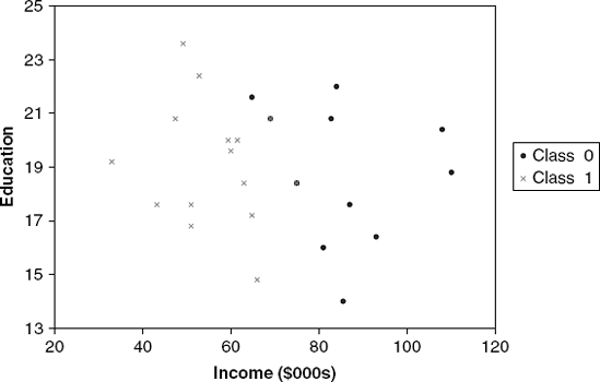
Unlike models that assume a particular relationship between the response and predictors (e.g., a linear relationship such as in linear regression and linear discriminant analysis), classification and regression trees are nonlinear and non-parametric. This allows for a wide range of relationships between the predictors and the response. However, this can also be a weakness: Since the splits are done on single predictors rather than on combinations of predictors, the tree is likely to miss relationships between predictors, in particular linear structures such as those in linear or logistic regression models. Classification trees are useful classifiers in cases where horizontal and vertical splitting of the predictor space adequately divides the classes. But consider, for instance, a dataset with two predictors and two classes, where separation between the two classes is most obviously achieved by using a diagonal line (as shown in Figure 9.18). A classification tree is therefore expected to have lower performance than methods such as discriminant analysis. One way to improve performance is to create new predictors that are derived from existing predictors, which can capture hypothesized relationships between predictors (similar to interactions in regression models).
Another performance issue with classification trees is that they require a large dataset in order to construct a good classifier. Recently, Breiman and Cutler introduced random forests,[19] an extension to classification trees that tackles these issues. The basic idea is to create multiple classification trees from the data (and thus obtain a "forest") and combine their output to obtain a better classifier.
An appealing feature of trees is that they handle missing data without having to impute values or delete observations with missing values. The method can be extended to incorporate an importance ranking for the variables in terms of their impact on the quality of the classification. From a computational aspect, trees can be relatively expensive to grow because of the multiple sorting involved in computing all possible splits on every variable. Pruning the data using the validation set adds further computation time. Finally, a very important practical advantage of trees is the transparent rules that they generate. Such transparency is often useful in managerial applications.
9.1 Competitive Auctions on
eBay.com. The file eBayAuctions.xls contains information on 1972 auctions transacted oneBay.comduring May-June 2004. The goal is to use these data to build a model that will classify competitive auctions from noncompetitive ones. A competitive auction is defined as an auction with at least two bids placed on the item auctioned. The data include variables that describe the item (auction category), the seller (his/her eBay rating), and the auction terms that the seller selected (auction duration, opening price, currency, day-of-week of auction close). In addition, we have the price at which the auction closed. The goal is to predict whether or not the auction will be competitive.Data Preprocessing. Create dummy variables for the categorical predictors. These include Category (18 categories), Currency (USD, GBP, Euro), EndDay (Monday-Sunday), and Duration (1, 3, 5, 7, or 10 days). Split the data into training and validation datasets using a 60% : 40% ratio.
Fit a classification tree using all predictors, using the best pruned tree. To avoid overfitting, set the minimum number of observations in a leaf node to 50. Also, set the maximum number of levels to be displayed at seven (the maximum allowed in XLminer). To remain within the limitation of 30 predictors, combine some of the categories of categorical predictors. Write down the results in terms of rules.
Is this model practical for predicting the outcome of a new auction?
Describe the interesting and uninteresting information that these rules provide.
Fit another classification tree (using the best-pruned tree, with a minimum number of observations per leaf node = 50 and maximum allowed number of displayed levels), this time only with predictors that can be used for predicting the outcome of a new auction. Describe the resulting tree in terms of rules. Make sure to report the smallest set of rules required for classification.
Plot the resulting tree on a scatterplot: Use the two axes for the two best (quantitative) predictors. Each auction will appear as a point, with coordinates corresponding to its values on those two predictors. Use different colors or symbols to separate competitive and noncompetitive auctions. Draw lines (you can sketch these by hand or use Excel) at the values that create splits. Does this splitting seem reasonable with respect to the meaning of the two predictors? Does it seem to do a good job of separating the two classes?
Examine the lift chart and the classification table for the tree. What can you say about the predictive performance of this model?
Based on this last tree, what can you conclude from these data about the chances of an auction obtaining at least two bids and its relationship to the auction settings set by the seller (duration, opening price, ending day, currency)? What would you recommend for a seller as the strategy that will most likely lead to a competitive auction?
9.2 Predicting Delayed Flights. The file FlightDelays.xls contains information on all commercial flights departing the Washington, D.C., area and arriving at New York during January 2004. For each flight there is information on the departure and arrival airports, the distance of the route, the scheduled time and date of the flight, and so on. The variable that we are trying to predict is whether or not a flight is delayed. A delay is defined as an arrival that is at least 15 minutes later than scheduled.
Data Preprocessing. Create dummies for day of week, carrier, departure airport, and arrival airport. This will give you 17 dummies. Bin the scheduled departure time into 2hour bins (in XLMiner use Data Utilities > Bin Continuous Data and select 8 bins with equal width). After binning DEP TIME into 8 bins, this new variable should be broken down into 7 dummies (because the effect will not be linear due to the morning and afternoon rush hours). This will avoid treating the departure time as a continuous predictor because it is reasonable that delays are related to rush-hour times. Partition the data into training and validation sets.
Fit a classification tree to the flight delay variable using all the relevant predictors. Do not include DEP TIME (actual departure time) in the model because it is unknown at the time of prediction (unless we are doing our predicting of delays after the plane takes off, which is unlikely). In the third step of the classification tree menu, choose "Maximum # levels to be displayed = 6". Use the best pruned tree without a limitation on the minimum number of observations in the final nodes. Express the resulting tree as a set of rules.
If you needed to fly between DCA and EWR on a Monday at 7 am, would you be able to use this tree? What other information would you need? Is it available in practice? What information is redundant?
Fit another tree, this time excluding the day-of-month predictor. (Why?) Select the option of seeing both the full tree and the best pruned tree. You will find that the best pruned tree contains a single terminal node.
How is this tree used for classification? (What is the rule for classifying?)
To what is this rule equivalent?
Examine the full tree. What are the top three predictors according to this tree?
Why, technically, does the pruned tree result in a tree with a single node?
What is the disadvantage of using the top levels of the full tree as opposed to the best pruned tree?
Compare this general result to that from logistic regression in the example in Chapter 10. What are possible reasons for the classification tree's failure to find a good predictive model?
9.3 Predicting Prices of Used Cars (Regression Trees). The file ToyotaCorolla.xls contains the data on used cars (Toyota Corolla) on sale during late summer of 2004 in The Netherlands. It has 1436 observations containing details on 38 attributes, including Price, Age, Kilometers, HP, and other specifications. The goal is to predict the price of a used Toyota Corolla based on its specifications. (The example in Section 9.8 is a subset of this dataset.)
Data Preprocessing. Create dummy variables for the categorical predictors (Fuel Type and Color). Split the data into training (50%), validation (30%), and test (20%) datasets.
Run a regression tree (RT) using the prediction menu in XLMiner with the output variable Price and input variables Age_08_04, KM, Fuel_Type, HP, Automatic, Doors, Quarterly_Tax, Mfg_Guarantee, Guarantee_Period, Airco, Automatic_Airco, CD_Player, Powered_Windows, Sport_Model, and Tow_Bar. Normalize the variables. Keep the minimum number of observations in a terminal node to 1 and the scoring option to Full Tree, to make the run least restrictive.
Which appear to be the three or four most important car specifications for predicting the car's price?
Compare the prediction errors of the training, validation, and test sets by examining their RMS error and by plotting the three boxplots. What is happening with the training set predictions? How does the predictive performance of the test set compare to the other two? Why does this occur?
How can we achieve predictions for the training set that are not equal to the actual prices?
If we used the best pruned tree instead of the full tree, how would this affect the predictive performance for the validation set? (Hint: Does the full tree use the validation data?)
Let us see the effect of turning the price variable into a categorical variable. First, create a new variable that categorizes price into 20 bins. Use Data Utilities > Bin Continuous Data to categorize Price into 20 bins of equal intervals (leave all other options at their default). Now repartition the data keeping Binned Price instead of Price. Run a classification tree (CT) using the Classification menu of XLMiner with the same set of input variables as in the RT, and with Binned Price as the output variable. Keep the minimum number of observations in a terminal node to 1 and uncheck the Prune Tree option, to make the run least restrictive. Select "Normalize input data."
Compare the tree generated by the CT with the one generated by the RT. Are they different? (Look at structure, the top predictors, size of tree, etc.) Why?
Predict the price, using the RT and the CT, of a used Toyota Corolla with the specifications listed in Table 9.3.
Compare the predictions in terms of the variables that were used, the magnitude of the difference between the two predictions, and the advantages and disadvantages of the two methods.
[16] Data Mining for Business Intelligence, By Galit Shmueli, Nitin R. Patel, and Peter C. Bruce
[17] This is a difference between CART and C4.5; the former performs only binary splits, leading to binary trees, whereas the latter performs splits that are as large as the number of categories, leading to "bushlike" structures.
[18] XLMiner uses a variant of the Gini index called the delta splitting rule; for details, see XLMiner documentation.
[19] For further details on random forests see www.stat.berkeley.edu/users/breiman/RandomForests/cc_home.htm