A large Toyota car dealership offers purchasers of new Toyota cars the option to buy their used car as part of a trade-in. In particular, a new promotion promises to pay high prices for used Toyota Corolla cars for purchasers of a new car. The dealer then sells the used cars for a small profit. To ensure a reasonable profit, the dealer needs to be able to predict the price that the dealership will get for the used cars. For that reason, data were collected on all previous sales of used Toyota Corollas at the dealership. The data include the sales price and other information on the car, such as its age, mileage, fuel type, and engine size. A description of each of these variables is given in Table 6.1. A sample of this dataset is shown in Table 6.2.

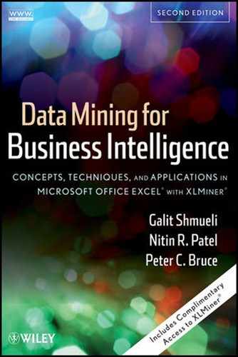
The total number of records in the dataset is 1000 cars (we use the first 1000 cars from the dataset ToyotoCorolla.xls). After partitioning the data into training and validation sets (at a 60% : 40% ratio), we fit a multiple linear regression model between price (the dependent variable) and the other variables (as predictors) using the training set only. Figure 6.1 shows the estimated coefficients (as computed by XLMiner). Notice that the Fuel Type predictor has three categories (Petrol, Diesel, and CNG), and we therefore have two dummy variables in the model [e.g., Petrol (0/1) and Diesel (0/1); the third, CNG (0/1), is redundant given the information on the first two dummies]. These coefficients are then used to predict prices of used Toyota Corolla cars based on their age, mileage, and so on. Figure 6.2 shows a sample of 20 of the predicted prices for cars in the validation set, using the estimated model. It gives the predictions and their errors (relative to the actual prices) for these 20 cars. On the right we get overall measures of predictive accuracy. Note that the average error is $111. A boxplot of the residuals (Figure 6.3) shows that 50% of the errors are approximately between ±$850. This might be small relative to the car price but should be taken into account when considering the profit. Such measures are used to assess the predictive performance of a model and to compare models. We discuss such measures in the next section. This example also illustrates the point about the relaxation of the normality assumption. A histogram or probability plot of prices shows a right-skewed distribution. In a classical modeling case where the goal is to obtain a good fit to the data, the dependent variable would be transformed (e.g., by taking a natural log) to achieve a more "normal" variable. Although the fit of such a model to the training data is expected to be better, it will not necessarily yield a significant predictive improvement. In this example the average error in a model of log(price) is −$160, compared to −$111 in the original model for price.

Figure 6.1. ESTIMATED COEFFICIENTS FOR REGRESSION MODEL OF PRICE VS. CAR ATTRIBUTES

Figure 6.2. (A) PREDICTED PRICES (AND ERRORS) FOR 20 CARS IN VALIDATION SET AND (B) SUMMARY PREDICTIVE MEASURES FOR ENTIRE VALIDATION SET

Figure 6.3. BOXPLOT OF MODEL RESIDUALS (BASED ON VALIDATION SET)

A frequent problem in data mining is that of using a regression equation to predict the value of a dependent variable when we have many variables available to choose as predictors in our model. Given the high speed of modern algorithms for multiple linear regression calculations, it is tempting in such a situation to take a kitchen-sink approach: Why bother to select a subset? Just use all the variables in the model. There are several reasons why this could be undesirable.

The last two points mean that there is a trade-off between too few and too many predictors. In general, accepting some bias can reduce the variance in predictions. This bias–variance trade-off is particularly important for large numbers of predictors because in that case it is very likely that there are variables in the model that have small coefficients relative to the standard deviation of the noise and also exhibit at least moderate correlation with other variables. Dropping such variables will improve the predictions, as it will reduce the prediction variance. This type of bias–variance trade-off is a basic aspect of most data mining procedures for prediction and classification. In light of this, methods for reducing the number of predictors p to a smaller set are often used.

The first step in trying to reduce the number of predictors should always be to use domain knowledge. It is important to understand what the various predictors are measuring and why they are relevant for predicting the response. With this knowledge the set of predictors should be reduced to a sensible set that reflects the problem at hand. Some practical reasons for predictor elimination are expense of collecting this information in the future, inaccuracy, high correlation with another predictor, many missing values, or simply irrelevance. Also helpful in examining potential predictors are summary statistics and graphs, such as frequency and correlation tables, predictor-specific summary statistics and plots, and missing value counts.

The next step makes use of computational power and statistical significance. In general, there are two types of methods for reducing the number of predictors in a model. The first is an exhaustive search for the "best" subset of predictors by fitting regression models with all the possible combinations of predictors. The second is to search through a partial set of models. We describe these two approaches next.

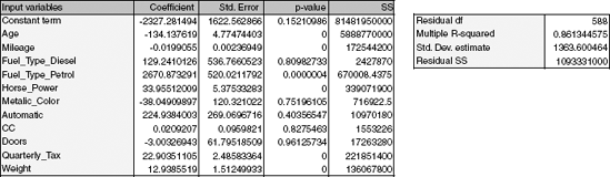
Exhaustive Search The idea here is to evaluate all subsets. Since the number of subsets for even moderate values of p is very large, we need some way to examine the most promising subsets and to select from them. Criteria for evaluating and comparing models are based on the fit to the training data. One popular criterion is the adjusted R², which is defined as

where R², is the proportion of explained variability in the model (in a model with a single predictor, this is the squared correlation). Like R², higher values of adjusted R² indicate better fit. Unlike R², which does not account for the number of predictors used, adjusted R² uses a penalty on the number of predictors. This avoids the artificial increase in R² that can result from simply increasing the number of predictors but not the amount of information. It can be shown that using R²_adj to choose a subset is equivalent to picking the subset that minimizes σ².

Another criterion that is often used for subset selection is known as Mallow's C_p. This criterion assumes that the full model (with all predictors) is unbiased, although it may have predictors that if dropped would reduce prediction variability. With this assumption we can show that if a subset model is unbiased, the average C_p value equals the number of parameters p+1 (= number of predictors +1), the size of the subset. So a reasonable approach to identifying subset models with small bias is to examine those with values of C_p that are near p+ 1. C_p is also an estimate of the error^[9] for predictions at the x values observed in the training set. Thus, good models are those that have values of C_p near p+ 1 and that have small p (i.e., are of small size). C_p is computed from the formula

where σ²_full is the estimated value of σ in the full model that includes all predictors, and SSR is the sum of squares of Regression given in the ANOVA table. It is important to remember that the usefulness of this approach depends heavily on the reliability of the estimate of σ²for the full model. This requires that the training set contain a large number of observations relative to the number of predictors. Finally, a useful point to note is that for a fixed size of subset, R², R_adj² and C_p all select the same subset. In fact, there is no difference between them in the order of merit they ascribe to subsets of a fixed size.

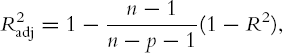
Figure 6.4 gives the results of applying an exhaustive search on the Toyota Corolla price data (with the 11 predictors). It reports the best model with a single predictor, 2 predictors, and so on. It can be seen that the R²_adj increases until 6 predictors are used (number of coefficients = 7) and then stabilizes. The C_p indicates that a model with 9–11 predictors is good. The dominant predictor in all models is the age of the car, with horsepower and mileage playing important roles as well.

Figure 6.4. EXHAUSTIVE SEARCH RESULT FOR REDUCING PREDICTORS IN TOYOTA COROLLA EXAMPLE

Popular Subset Selection Algorithms The second method of finding the best subset of predictors relies on a partial, iterative search through the space of all possible regression models. The end product is one best subset of predictors (although there do exist variations of these methods that identify several close-to-best choices for different sizes of predictor subsets). This approach is computationally cheaper, but it has the potential of missing "good" combinations of predictors. None of the methods guarantee that they yield the best subset for any criterion, such as adjusted R². They are reasonable methods for situations with large numbers of predictors, but for moderate numbers of predictors the exhaustive search is preferable.

Three popular iterative search algorithms are forward selection, backward elimination, and stepwise regression. In forward selection we start with no predictors and then add predictors one by one. Each predictor added is the one (among all predictors) that has the largest contribution to R² on top of the predictors that are already in it. The algorithm stops when the contribution of additional predictors is not statistically significant. The main disadvantage of this method is that the algorithm will miss pairs or groups of predictors that perform very well together but perform poorly as single predictors. This is similar to interviewing job candidates for a team project one by one, thereby missing groups of candidates who perform superiorly together, but poorly on their own.

In backward elimination we start with all predictors and then at each step eliminate the least useful predictor (according to statistical significance). The algorithm stops when all the remaining predictors have significant contributions. The weakness of this algorithm is that computing the initial model with all predictors can be time consuming and unstable. Stepwise regression is like forward selection except that at each step we consider dropping predictors that are not statistically significant, as in backward elimination.

Note: In XLMiner, unlike other popular software packages (SAS, Minitab, etc.), these three algorithms yield a table similar to the one that the exhaustive search yields rather than a single model. This allows the user to decide on the subset size after reviewing all possible sizes based on criteria such as R_adj² and C_p.

Figure 6.5. BACKWARD ELIMINATION RESULT FOR REDUCING PREDICTORS IN TOYOTA COROLLA EXAMPLE

For the Toyota Corolla price example, forward selection yields exactly the same results as those found in an exhaustive search: For each number of predictors the same subset is chosen (it therefore gives a table identical to the one in Figure 6.4). Notice that this will not always be the case. In comparison, backward elimination starts with the full model and then drops predictors one by one in this order: Doors, CC, Diesel, Metallic, Automatic, QuartTax, Petrol, Weight, and Age (see Figure 6.5). The R_adj² and C_p measures indicate exactly the same subsets as those suggested by the exhaustive search. In other words, it correctly identifies Doors, CC, Diesel, Metallic, and Automatic as the least useful predictors. Backward elimination would yield a different model than that of the exhaustive search only if we decided to use fewer than six predictors. For instance, if we were limited to two predictors, backward elimination would choose Age and Weight, whereas an exhaustive search shows that the best pair of predictors is actually Age and HP.

The results for stepwise regression can be seen in Figure 6.6. It chooses the same subsets as forward selection for subset sizes of 1–7 predictors. However, for 8–10 predictors, it chooses a different subset than that chosen using the other methods: It decides to drop Doors, Quart Tax, and Weight. This means that it fails to detect the best subsets for 8–10 predictors. R_adj² is largest at 6 predictors (the same 6 as were selected by the other models), but C_p indicates that the full model with 11 predictors is the best fit.

Figure 6.6. STEPWISE SELECTION RESULT FOR REDUCING PREDICTORS IN TOYOTA COROLLA EXAMPLE

This example shows that the search algorithms yield fairly good solutions, but we need to carefully determine the number of predictors to retain. It also shows the merits of running a few searches and using the combined results to determine the subset to choose. There is a popular (but false) notion that stepwise regression is superior to backward elimination and forward selection because of its ability to add and to drop predictors. This example shows clearly that it is not always so.

Finally, additional ways to reduce the dimension of the data are by using principal components (Chapter 4) and regression trees (Chapter 9).