
In this chapter we describe the context of business time series forecasting and introduce the main approaches that are detailed in the next chapters (in particular, regression-based forecasting and smoothing-based methods). Our focus is on forecasting future values of a single time series. We discuss the difference between the predictive nature of time series forecasting versus the descriptive or explanatory task of time series analysis. A general discussion of combining forecasting methods or results for added precision follows. Next, we present a time series in terms of four components (level, trend, seasonality, and noise) and present methods for visualizing the different components and for exploring time series data. We close with a discussion of data partitioning (to create training and validation sets), which is performed differently than cross-sectional data partitioning.
Time series forecasting is performed in nearly every organization that works with quantifiable data. Retail stores use it to forecast sales. Energy companies use it to forecast reserves, production, demand, and prices. Educational institutions use it to forecast enrollment. Governments use it to forecast tax receipts and spending. International financial organizations such as the World Bank and International Monetary Fund use it to forecast inflation and economic activity. Transportation companies use time series forecasting to forecast future travel. Banks and lending institutions use it (sometimes badly!) to forecast new home purchases. And venture capital firms use it to forecast market potential and to evaluate business plans.
Previous chapters in this book deal with classifying and predicting data where time is not a factor (in the sense that it is not treated differently from other variables), and where the order of measurements in time does not matter. These are typically called cross-sectional data. In contrast, this chapter deals with a different type of data: time series.
With today's technology, many time series are recorded on very frequent time scales. Stock data are available at ticker level. Purchases at online and offline stores are recorded in real time. Although data might be available at a very frequent scale, for the purpose of forecasting it is not always preferable to use this time scale. In considering the choice of time scale, one must consider the scale of the required forecasts and the level of noise in the data. For example, if the goal is to forecast next-day sales at a grocery store, using minute-by-minute sales data are likely to be less useful for forecasting than using daily aggregates. The minute-by-minute series will contain many sources of noise (e.g., variation by peak and nonpeak shopping hours) that degrade its forecasting power, and these noise errors, when the data are aggregated to a coarser level, are likely to average out.
The focus in this part of the book is on forecasting a single time series. In some cases multiple time series are to be forecasted (e.g., the monthly sales of multiple products). Even when multiple series are being forecasted, the most popular forecasting practice is to forecast each series individually. The advantage of single-series forecasting is simplicity. The disadvantage is that it does not take into account possible relationships between series. The statistics literature contains models for multivariate time series that directly model the cross correlations between series. Such methods tend to make restrictive assumptions about the data and the cross-series structure, and they also require statistical expertise for estimation and maintenance. Econometric models often include information from one or more series as inputs into another series. However, such models are based on assumptions of causality that are based on theoretical models. An alternative approach is to capture the associations between the series of interest and external information more heuristically. An example is using the sales of lipstick to forecast some measure of the economy, based on the observation by Ronald Lauder, chairman of Estee Lauder, that lipstick sales tend to increase before tough economic times (a phenomenon called the "leading lipstick indicator").
As with cross-sectional data, modeling time series data is done for either explanatory or predictive purposes. In explanatory modeling, or time series analysis, a time series is modeled to determine its components in terms of seasonal patterns, trends, relation to external factors, and the like. These can then be used for decision making and policy formulation. In contrast, time series forecasting uses the information in a time series (and perhaps other information) to forecast future values of that series. The difference between the goals of time series analysis and time series forecasting leads to differences in the type of methods used and in the modeling process itself. For example, in selecting a method for explaining a time series, priority is given to methods that produce explainable results (rather than black-box methods) and to models based on causal arguments. Furthermore, explaining can be done in retrospect, while forecasting is prospective in nature. This means that explanatory models might use "future" information (e.g., averaging the values of yesterday, today, and tomorrow to obtain a smooth representation of today's value) whereas forecasting models cannot.
The focus in this chapter is on time series forecasting, where the goal is to predict future values of a time series. For information on time series analysis see Chatfield (2003).
In this part of the book we focus on two main types of forecasting methods that are popular in business applications. Both are versatile and powerful, yet relatively simple to understand and deploy. One type of forecasting tool is multiple linear regression, where the user specifies a certain model and then estimates it from the time series. The other is the more data-driven tool of smoothing, where the method learns patterns from the data. Each of the two types of tools has advantages and disadvantages, as detailed in Chapters 16 and 17. We also note that data mining methods such as neural networks and others that are intended for cross-sectional data are also sometimes used for time series forecasting, especially for incorporating external information into the forecasts.
Before a discussion of specific forecasting methods in the following two chapters, it should be noted that a popular approach for improving predictive performance is to combine forecasting methods. Combining methods can be done via two-level (or multilevel) forecasters, where the first method uses the original time series to generate forecasts of future values, and the second method uses the residuals from the first model to generate forecasts of future forecast errors, thereby "correcting" the first level forecasts. We describe two-level forecasting in Section 16.4. Another combination approach is via "ensembles," where multiple methods are applied to the time series, and their resulting forecasts are averaged in some way to produce the final forecast. Combining methods can take advantage of the strengths of different forecasting methods to capture different aspects of the time series (also true in cross-sectional data). The averaging across multiple methods can lead to forecasts that are more robust and of higher precision.
In both types of forecasting methods (regression models and smoothing) and in general, it is customary to dissect a time series into four components: level, trend, seasonality, and noise. The first three components are assumed to be invisible, as they characterize the underlying series, which we only observe with added noise. Level describes the average value of the series, trend is the change in the series from one period to the next, and seasonality describes a short-term cyclical behavior of the series that can be observed several times within the given series. Finally, noise is the random variation that results from measurement error or other causes not accounted for. It is always present in a time series to some degree.
In order to identify the components of a time series, the first step is to examine a time plot. In its simplest form, a time plot is a line chart of the series values over time, with temporal labels (e.g., calendar date) on the horizontal axis. To illustrate this, consider the following example.
Amtrak, a U.S. railway company, routinely collects data on ridership. Here we focus on forecasting future ridership using the series of monthly ridership between January 1991 and March 2004. These data are publicly available at http://www.forecastingprinciples.com (click on Data, and select Series M-34 from the T-Competition Data).
A time plot for monthly Amtrak ridership series is shown in Figure 15.1. Note that the values are in thousands of riders. Looking at the time plot reveals the nature of the series components: the overall level is around 1,800,000 passengers per month. A slight U-shaped trend is discernible during this period, with pronounced annual seasonality, with peak travel during summer (July and August).
A second step in visualizing a time series is to examine it more carefully. A few tools are useful:
Zoom in: Zooming in to a shorter period within the series can reveal patterns that are hidden when viewing the entire series. This is especially important when the time series is long. Consider a series of the daily number of vehicles passing through the Baregg tunnel in Switzerland (data are available in the same location as the Amtrak Ridership data; series D028). The series from Nov. 1, 2003 to Nov. 16, 2005 is shown in the top panel of Figure 15.2. Zooming in to a 4-month period (bottom panel) reveals a strong day-of-week pattern that was not visible in the initial time plot of the complete time series.
Change Scale of Series: In order to better identify the shape of a trend, it is useful to change the scale of the series. One simple option is to change the vertical scale to a logarithmic scale (in Excel 2003 double-click on the y-axis labels and check "logarithmic scale"; in Excel 2007 select Layout> Axes > Axes > Primary Vertical Axis and click "logarithmic scale" in the Format Axis menu). If the trend on the new scale appears more linear, then the trend in the original series is closer to an exponential trend.
Add Trend Lines: Another possibility for better capturing the shape of the trend is to add a trend line (Excel 2003: Chart> Add Trendline; Excel 2007: Layout> Analysis > Trendline). By trying different trend lines one can see what type of trend (e.g., linear, exponential, cubic) best approximates the data.
Suppress Seasonality: It is often easier to see trends in the data when season-ality is suppressed. Suppressing seasonality patterns can be done by plotting the series at a cruder time scale (e.g., aggregating monthly data into years). Another popular option is to use moving-average plots. We will discuss these in Section 17.2.

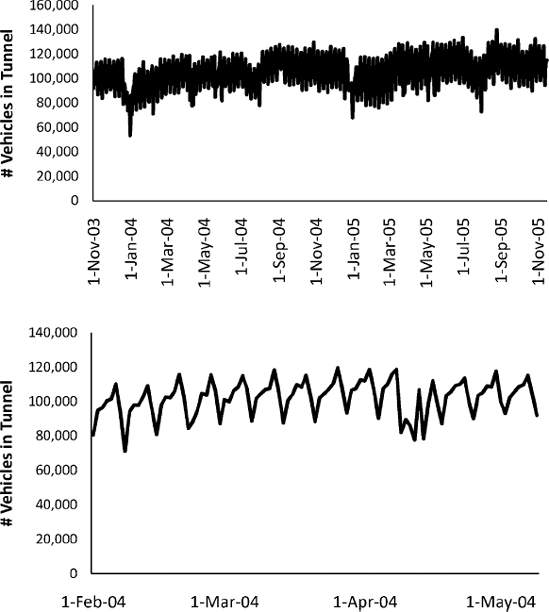
Figure 15.2. TIME PLOTS OF THE DAILY NUMBER OF VEHICLES PASSING THROUGH THE BAREGG TUNNEL (SWITZERLAND). THE BOTTOM PANEL ZOOMS IN TO A 4-MONTH PERIOD, REVEALING A DAY-OF-WEEK PATTERN
Continuing our example of Amtrak ridership, the plots in Figure 15.3 help make the series' components more visible.
Some forecasting methods directly model these components by making assumptions about their structure. For example, a popular assumption about trend is that it is linear or exponential over the given time period or part of it. Another common assumption is about the noise structure: Many statistical methods assume that the noise follows a normal distribution. The advantage of methods that rely on such assumptions is that when the assumptions are reasonably met, the resulting forecasts will be more robust and the models more understandable. Other forecasting methods, which are data adaptive, make fewer assumptions about the structure of these components and instead try to estimate them only from the data. Data-adaptive methods are advantageous when such assumptions are likely to be violated, or when the structure of the time series changes over time. Another advantage of many data-adaptive methods is their simplicity and computational efficiency.

Figure 15.3. PLOTS THAT ENHANCE THE DIFFERENT COMPONENTS OF THE TIME SERIES. TOP: ZOOM IN TO 3 YEARS OF DATA. BOTTOM: ORIGINAL SERIES WITH OVERLAID POLYNOMIAL TREND LINE
A key criterion for choosing between model-driven and data-driven forecasting methods is the nature of the series in terms of global versus local patterns. A global pattern is one that is relatively constant throughout the series. An example is a linear trend throughout the entire series. In contrast, a local pattern is one that occurs only in a short period of the data, and then changes. An example is a trend that is approximately linear within four neighboring time points, but the trend size (slope) changes slowly over time.
Model-driven methods are generally preferable for forecasting series with global patterns, as they use all the data to estimate the global pattern. For a local pattern, a model-driven model would require specifying how and when the patterns change, which is usually impractical and often unknown. Therefore, data-driven methods are preferable for local patterns. Such methods "learn" patterns from the data, and their memory length can be set to best adapt to the rate of change in the series. Patterns that change quickly warrant a "short memory," whereas patterns that change slowly warrant a "long memory." In conclusion, the time plot should be used not only to identify the time series component but also the global/local nature of the trend and seasonality.
As in the case of cross-sectional data, in order to avoid overfitting and to be able to assess the predictive performance of the model on new data, we first partition the data into a training set and a validation set (and perhaps an additional test set). However, there is one important difference between data partitioning in cross-sectional and time series data. In cross-sectional data the partitioning is usually done randomly, with a random set of observations designated as training data and the remainder as validation data. However, in time series a random partition would create two time series with "holes!" Nearly all standard forecasting methods cannot handle time series with missing values. Therefore, we partition a time series into training and validation sets differently. The series is trimmed into two periods; the earlier period is set as the training data and the later period as the validation data. Methods are then trained on the earlier periods, and their predictive performance assessed on the later period. Evaluation metrics typically use the same metrics used in cross-sectional evaluation (see Chapter 5.3) with MAPE and RMSE being the most popular metrics in practice. In evaluating and comparing forecasting methods, another important tool is visualization: Examining time plots of the actual and predicted series can shed light on performance and hint toward possible improvements.
One last important difference between cross-sectional and time series partitioning occurs when creating the actual forecasts. Before attempting to forecast future values of the series, the training and validation sets are recombined into one long series, and the chosen method/model is rerun on the complete data. This final model is then used to forecast future values. The three advantages in recombining are: (1) The validation set, which is the most recent period, usually contains the most valuable information in terms of being the closest in time to the forecasted period. (2) With more data (the complete time series, compared to only the training set), some models can be estimated more accurately. (3) If only the training set is used to generate forecasts, then it will require forecasting farther into the future (e.g., if the validation set contains 4 time points, forecasting the next observation will require a 5-step-ahead forecast from the training set).
Note
In XLMiner, partitioning a time series is performed within the Time Series menu. Figure 15.4 shows a screenshot of the time series partitioning dialog box. After the final model is chosen, the same model should be rerun on the original, unpartitioned series in order to obtain forecasts. XLMiner will only generate future forecasts if it is run on an unpartitioned series.

15.1 Impact of September 11 on Air Travel in the United States: The Research and Innovative Technology Administration's Bureau of Transportation Statistics (BTS) conducted a study to evaluate the impact of the September 11, 2001, terrorist attack on U.S. transportation. The study report and the data can be found at
http://www.bts.gov/publications/estimated_impacts_of_9_11_on_us_travel. The goal of the study was stated as follows:The purpose of this study is to provide a greater understanding of the passenger travel behavior patterns of persons making long distance trips before and after 9/11.
The report analyzes monthly passenger movement data between January 1990 and May 2004. Data on three monthly time series are given in file Sept11Travel.xls for this period: (1) actual airline revenue passenger miles (Air), (2) rail passenger miles (Rail), and (3) vehicle miles traveled (Car).
In order to assess the impact of September 11, BTS took the following approach: Using data before September 11, it forecasted future data (under the assumption of no terrorist attack). Then, BTS compared the forecasted series with the actual data to assess the impact of the event. Our first step, therefore, is to split each of the time series into two parts: pre-and post-September 11. We now concentrate only on the earlier time series.
Is the goal of this study explanatory or predictive?
Plot each of the three preevent time series (Air, Rail, Car).
What time series components appear from the plot?
What type of trend appears? Change the scale of the series, add trend lines, and suppress seasonality to better visualize the trend pattern.
15.2 Performance on Training and Validation Data: Two different models were fit to the same time series. The first 100 time periods were used for the training set and the last 12 periods were treated as a hold-out set. Assume that both models make sense practically and fit the data pretty well. Below are the RMSE values for each of the models:
Training Set
Validation Set
Model A
543
20
Model B
869
14
Which model appears more useful for explaining the different components of this time series? Why?
Which model appears to be more useful for forecasting purposes? Why?
15.3 Forecasting Department Store Sales: The file DepartmentStoreSales.xls contains data on the quarterly sales for a department store over a 6-year period (data courtesy of Chris Albright).
15.4 Shipments of Household Appliances: The file ApplianceShipments.xls contains the series of quarterly shipments (in million $) of U.S. household appliances between 1985 and 1989 (data courtesy of Ken Black).
Create a well-formatted time plot of the data.
Which of the four components (level, trend, seasonality, noise) seem to be present in this series?
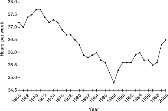
15.5 Analysis of Canadian Manufacturing Workers Workhours: The time series plot in menu. Figure 15.5 describes the average annual number of weekly hours spent by Canadian manufacturing workers (data are available in CanadianWorkHours.xls—thanks to Ken Black for these data).
Reproduce the time plot.
Which of the four components (level, trend, seasonality, noise) appear to be present in this series?
15.6 Souvenir Sales: The file SouvenirSales.xls contains monthly sales for a souvenir shop at a beach resort town in Queensland, Australia, between 1995 and 2001. [Source: R. J. Hyndman, Time Series Data Library,
http://www.robjhyndman.com/TSDL; accessed on December 20, 2009.]Back in 2001, the store wanted to use the data to forecast sales for the next 12 months (year 2002). They hired an analyst to generate forecasts. The analyst first partitioned the data into training and validation sets, with the validation set containing the last 12 months of data (year 2001). She then fit a regression model to sales, using the training set.
Create a well-formatted time plot of the data.
Change the scale on the x axis, or on the y axis, or on both to log scale in order to achieve a linear relationship. Select the time plot that seems most linear.
Comparing the two time plots, what can be said about the type of trend in the data?
Why were the data partitioned? Partition the data into the training and validation set as explained above.
15.7 Forecasting Shampoo Sales: The file ShampooSales.xls contains data on the monthly sales of a certain shampoo over a 3-year period. (Source: R. J. Hyndman, Time Series Data Library,
http://www.robjhyndman.com/TSDL; accessed on December 28, 2009.)Create a well-formatted time plot of the data.
Which of the four components (level, trend, seasonality, noise) seem to be present in this series?
Do you expect to see seasonality in sales of shampoo? Why?
If the goal is forecasting sales in future months, which of the following steps should be taken? (choose one or more)
Partition the data into training and validation sets.
Tweak the model parameters to obtain good fit to the validation data.
Look at MAPE and RMSE values for the training set.
Look at MAPE and RMSE values for the validation set.
[38] Data Mining for Business Intelligence, By Galit Shmueli, Nitin R. Patel, and Peter C. Bruce Statistics.com and Galit Shmueli