This chapter is about the popular unsupervised learning task of clustering, where the goal is to segment the data into a set of homogeneous clusters of observations for the purpose of generating insight. Clustering is used in a vast variety of business applications, from customized marketing to industry analysis. We describe two popular clustering approaches: hierarchical clustering and k-means clustering. In hierarchical clustering, observations are sequentially grouped to create clusters, based on distances between observations and distances between clusters. We describe how the algorithm works in terms of the clustering process and mention several common distance metrics used. Hierarchical clustering also produces a useful graphical display of the clustering process and results, called a dendrogram. We present dendrograms and illustrate their usefulness. k-means clustering is widely used in large dataset applications. In k-means clustering, observations are allocated to one of a prespecified set of clusters, according to their distance from each cluster. We describe the k-means clustering algorithm and its computational advantages. Finally, we present techniques that assist in generating insight from clustering results.
Cluster analysis is used to form groups or clusters of similar records based on several measurements made on these records. The key idea is to characterize the clusters in ways that would be useful for the aims of the analysis. This idea has been applied in many areas, including astronomy, archaeology, medicine, chemistry, education, psychology, linguistics, and sociology. Biologists, for example, have made extensive use of classes and subclasses to organize species. A spectacular success of the clustering idea in chemistry was Mendeleevo's periodic table of the elements.
One popular use of cluster analysis in marketing is for market segmentation: Customers are segmented based on demographic and transaction history information, and a marketing strategy is tailored for each segment. Another use is for market structure analysis: identifying groups of similar products according to competitive measures of similarity. In marketing and political forecasting, clustering of neighborhoods using U.S. postal zip codes has been used successfully to group neighborhoods by lifestyles. Claritas, a company that pioneered this approach, grouped neighborhoods into 40 clusters using various measures of consumer expenditure and demographics. Examining the clusters enabled Claritas to come up with evocative names, such as Bohemian Mix, Furs and Station Wagons, and Money and Brains, for the groups that captured the dominant lifestyles. Knowledge of lifestyles can be used to estimate the potential demand for products (such as sports utility vehicles) and services (such as pleasure cruises).
In finance, cluster analysis can be used for creating balanced portfolios: Given data on a variety of investment opportunities (e.g., stocks), one may find clusters based on financial performance variables such as return (daily, weekly, or monthly), volatility, beta, and other characteristics, such as industry and market capitalization. Selecting securities from different clusters can help create a balanced portfolio. Another application of cluster analysis in finance is for industry analysis: For a given industry, we are interested in finding groups of similar firms based on measures such as growth rate, profitability, market size, product range, and presence in various international markets. These groups can then be analyzed in order to understand industry structure and to determine, for instance, who is a competitor.
An interesting and unusual application of cluster analysis, described in Berry and Linoff (1997), is the design of a new set of sizes for army uniforms for women in the U.S. Army. The study came up with a new clothing size system with only 20 sizes, where different sizes fit different body types. The 20 sizes are combinations of five measurements: chest, neck, and shoulder circumference, sleeve outseam, and neck-to-buttock length [for further details, see McCullugh et al. (1998)]. This example is important because it shows how a completely new insightful view can be gained by examining clusters of records.
Cluster analysis can be applied to huge amounts of data. For instance, Internet search engines use clustering techniques to cluster queries that users submit. These can then be used for improving search algorithms. The objective of this chapter is to describe the key ideas underlying the most commonly used techniques for cluster analysis and to lay out their strengths and weaknesses.
Typically, the basic data used to form clusters are a table of measurements on several variables, where each column represents a variable and a row represents a record. Our goal is to form groups of records so that similar records are in the same group. The number of clusters may be prespecified or determined from the data.
Table 14.1 gives corporate data on 22 U.S. public utilities (the definition of each variable is given in the table footnote). We are interested in forming groups of similar utilities. The records to be clustered are the utilities, and the clustering will be based on the eight measurements on each utility. An example where clustering would be useful is a study to predict the cost impact of deregulation. To do the requisite analysis, economists would need to build a detailed cost model of the various utilities. It would save a considerable amount of time and effort if we could cluster similar types of utilities and build detailed cost models for just one "typical" utility in each cluster and then scale up from these models to estimate results for all utilities.
Table 14.1. DATA ON 22 PUBLIC UTILITIESa
Company | Fixed | RoR | Cost | Load | Demand | Sales | Nuclear | Fuel Cost |
|---|---|---|---|---|---|---|---|---|
Fixed = fixed-charge covering ratio (income/debt); RoR = rate of return on capital; Cost = cost per kilowatt capacity in place; Load = annual load factor; Demand = peak kilowatthour demand growth from 1974 to 1975; Sales = sales (kilowatthour use per year); Nuclear = percent nuclear; Fuel total fuel costs (cents per kilowatthour). | ||||||||
Arizona Public Service | 1.06 | 9.2 | 151 | 54.4 | 1.6 | 9,077 | 0 | 0.628 |
Boston Edison Co. | 0.89 | 10.3 | 202 | 57.9 | 2.2 | 5,088 | 25.3 | 1.555 |
Central Louisiana Co. | 1.43 | 15.4 | 113 | 53 | 3.4 | 9,212 | 0 | 1.058 |
Commonwealth Edison Co. | 1.02 | 11.2 | 168 | 56 | 0.3 | 6,423 | 34.3 | 0.7 |
Consolidated Edison Co. (NY) | 1.49 | 8.8 | 192 | 51.2 | 1 | 3,300 | 15.6 | 2.044 |
Florida Power & Light Co. | 1.32 | 13.5 | 111 | 60 | −2.2 | 11,127 | 22.5 | 1.241 |
Hawaiian Electric Co. | 1.22 | 12.2 | 175 | 67.6 | 2.2 | 7,642 | 0 | 1.652 |
Idaho Power Co. | 1.1 | 9.2 | 245 | 57 | 3.3 | 13,082 | 0 | 0.309 |
Kentucky Utilities Co. | 1.34 | 13 | 168 | 60.4 | 7.2 | 8,406 | 0 | 0.862 |
Madison Gas & Electric Co. | 1.12 | 12.4 | 197 | 53 | 2.7 | 6,455 | 39.2 | 0.623 |
Nevada Power Co. | 0.75 | 7.5 | 173 | 51.5 | 6.5 | 17,441 | 0 | 0.768 |
New England Electric Co. | 1.13 | 10.9 | 178 | 62 | 3.7 | 6,154 | 0 | 1.897 |
Northern States Power Co. | 1.15 | 12.7 | 199 | 53.7 | 6.4 | 7,179 | 50.2 | 0.527 |
Oklahoma Gas & Electric Co. | 1.09 | 12 | 96 | 49.8 | 1.4 | 9,673 | 0 | 0.588 |
Pacific Gas & Electric Co. | 0.96 | 7.6 | 164 | 62.2 | −0.1 | 6,468 | 0.9 | 1.4 |
Puget Sound Power & Light Co. | 1.16 | 9.9 | 252 | 56 | 9.2 | 15,991 | 0 | 0.62 |
San Diego Gas & Electric Co. | 0.76 | 6.4 | 136 | 61.9 | 9 | 5,714 | 8.3 | 1.92 |
The Southern Co. | 1.05 | 12.6 | 150 | 56.7 | 2.7 | 10,140 | 0 | 1.108 |
Texas Utilities Co. | 1.16 | 11.7 | 104 | 54 | −2.1 | 13,507 | 0 | 0.636 |
Wisconsin Electric Power Co. | 1.2 | 11.8 | 148 | 59.9 | 3.5 | 7,287 | 41.1 | 0.702 |
United Illuminating Co. | 1.04 | 8.6 | 204 | 61 | 3.5 | 6,650 | 0 | 2.116 |
Virginia Electric & Power Co. | 1.07 | 9.3 | 174 | 54.3 | 5.9 | 10,093 | 26.6 | 1.306 |
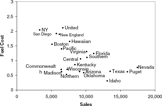
For simplicity, let us consider only two of the measurements: Sales and Fuel Cost. Figure 14.1 shows a scatterplot of these two variables, with labels marking each company. At first glance, there appear to be two or three clusters of utilities: one with utilities that have high fuel costs, a second with utilities that have lower fuel costs and relatively low sales, and a third with utilities with low fuel costs but high sales. We can therefore think of cluster analysis as a more formal algorithm that measures the distance between records, and according to these distances (here, two-dimensional distances) forms clusters.
There are two general types of clustering algorithms for a dataset of n records:
Hierarchical Methods Can be either agglomerative or divisive. Agglomerative methods begin with n clusters and sequentially merge similar clusters until a single cluster is left. Divisive methods work in the opposite direction, starting with one cluster that includes all observations. Hierarchical methods are especially useful when the goal is to arrange the clusters into a natural hierarchy.
Nonhierarchical Methods For example, k-means clustering. Using a prespecified number of clusters, the method assigns cases to each cluster. These methods are generally less computationally intensive and are therefore preferred with very large datasets.
We concentrate here on the two most popular methods: hierarchical agglomerative clustering and k-means clustering. In both cases we need to define two types of distances: distance between two records and distance between two clusters. In both cases there is a variety of metrics that can be used.
We denote by dij a distance metric, or dissimilarity measure, between records i and j. For record i we have the vector of p measurements (xi1, xi2, ..., xip), while for record j we have the vector of measurements (xj1, xj2, . . ., xp). For example, we can write the measurement vector for Arizona Public Service as [1.06, 9.2, 151, 54.4,1.6, 9077, 0, 0.628].
Distances can be defined in multiple ways, but, in general, the following properties are required:
The most popular distance measure is the Euclidean distance, dij, which between two cases, i and j, is defined by
For instance, the Euclidean distance between Arizona Public Service and Boston Edison Co. can be computed from the raw data by
The measure computed above is highly influenced by the scale of each variable, so that variables with larger scales (e.g., Sales) have a much greater influence over the total distance. It is therefore customary to normalize (or standardize) continuous measurements before computing the Euclidean distance. This converts all measurements to the same scale. Normalizing a measurement means subtracting the average and dividing by the standard deviation (normalized values are also called z scores). For instance, the figure for average sales across the 22 utilities is 8914.045 and the standard deviation is 3549.984. The normalized sales for Arizona Public Service is therefore (9077 – 8914.045)/3549.984) = 0.046.
Returning to the simplified utilities data with only two measurements (Sales and Fuel Cost), we first normalize the measurements (see Table 14.2), and then compute the Euclidean distance between each pair. Table 14.3 gives these pairwise distanced for the first 5 utilities. A similar table can be constructed for all 22 utilities.
Table 14.2. ORIGINAL AND NORMALIZED MEASUREMENTS FOR SALES AND FUEL COST
Company | Sales | Fuel Cost | NormSales | NormFuel |
|---|---|---|---|---|
Arizona Pulic Service | 9,077 | 0.628 | 0.0459 | −0.8537 |
Boston Edison Co. | 5,088 | 1.555 | −1.0778 | 0.8133 |
Central Louisiana Co. | 9,212 | 1.058 | 0.0839 | −0.0804 |
Commonwealth Edison Co. | 6,423 | 0.7 | −0.7017 | −0.7242 |
Consolidated Edison Co. (NY) | 3,300 | 2.044 | −1.5814 | 1.6926 |
Florida Power & Light Co. | 11,127 | 1.241 | 0.6234 | 0.2486 |
Hawaiian Electric Co. | 7,642 | 1.652 | −0.3583 | 0.9877 |
Idaho Power Co. | 13,082 | 0.309 | 1.1741 | −1.4273 |
Kentucky Utilities Co. | 8,406 | 0.862 | −0.1431 | −0.4329 |
Madison Gas & Electric Co. | 6,455 | 0.623 | −0.6927 | −0.8627 |
Nevada Power Co. | 17,441 | 0.768 | 2.4020 | −0.6019 |
New England Electric Co. | 6,154 | 1.897 | −0.7775 | 1.4283 |
Northem States Power Co. | 7,179 | 0.527 | −0.4887 | −1.0353 |
Oklahoma Gas & Electric Co. | 9,673 | 0.588 | 0.2138 | −0.9256 |
Pacific Gas & Electric Co. | 6,468 | 1.4 | −0.6890 | 0.5346 |
Puget Sound Power &Light Co. | 15.991 | 0.62 | 1.9935 | −0.8681 |
San Diego Gas & Electric Co. | 5,714 | 1.92 | −0.9014 | 1.4697 |
The Southern Co. | 10,140 | 1.108 | 0.3453 | 0.0095 |
Texas Utilities Co. | 13,507 | 0.636 | 1.2938 | −0.8393 |
Wisconsin Electric Power Co. | 7,287 | 0.702 | −0.4586 | −0.7206 |
United Illuminating Co. | 6,650 | 2.116 | −0.6378 | 1.8221 |
Virginia Electric & Power Co. | 10,093 | 1.306 | 0.3321 | 0.3655 |
Mean | 8,914.05 | 1.10 | 0.00 | 0.00 |
Standard deviation | 3,549.98 | 0.56 | 1.00 | 1.00 |
It is important to note that the choice of the distance measure plays a major role in cluster analysis. The main guideline is domain dependent: What exactly is being measured? How are the different measurements related? What scale should it be treated as (numerical, ordinal, or nominal)? Are there outliers? Finally, depending on the goal of the analysis, should the clusters be distinguished mostly by a small set of measurements, or should they be separated by multiple measurements that weight moderately?
Although Euclidean distance is the most widely used distance, it has three main features that need to be kept in mind. First, as mentioned above, it is highly scale dependent. Changing the units of one variable (e.g., from cents to dollars) can have a huge influence on the results. Standardizing is therefore a common solution. But unequal weighting should be considered if we want the clusters to depend more on certain measurements and less on others. The second feature of Euclidean distance is that it completely ignores the relationship between the measurements. Thus, if the measurements are in fact strongly correlated, a different distance (such as the statistical distance, described below) is likely to be a better choice. Third, Euclidean distance is sensitive to outliers. If the data are believed to contain outliers and careful removal is not a choice, the use of more robust distances (such as the Manhattan distance described below) is preferred.
Additional popular distance metrics often used (for reasons such as the ones above) are:
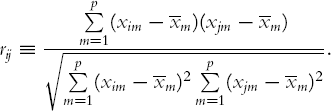
Correlation-Based Similarity Sometimes it is more natural or convenient to work with a similarity measure between records rather than distance, which measures dissimilarity. A popular similarity measure is the square of the correlation coefficient, r2ij where the correlation coefficient is defined by
Such measures can always be converted to distance measures. In the example above we could define a distance measure dj = 1 – ri2j.
Statistical Distance(also called Mahalanobis distance) This metric has an advantage over the other metrics mentioned in that it takes into account the correlation between measurements. With this metric, measurements that are highly correlated with other measurements do not contribute as much as those that are uncorrelated or mildly correlated. The statistical distance between records i and j is defined as
where xi and x j are p-dimensional vectors of the measurement values for records i and j, respectively; and S is the covariance matrix for these vectors. (The notation' denotes a transpose operation, which turns a column vector into a row vector.) S- is the inverse matrix of S, which is the p- dimension extension to division. For further information on statistical distance, see Chapter 12.
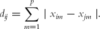
Manhattan Distance (city block) This distance looks at the absolute differences rather than squared differences, and is defined by
Maximum Coordinate Distance This distance looks only at the measurement on which records i and j deviate most. It is defined by
In the case of measurements with binary values, it is more intuitively appealing to use similarity measures than distance measures. Suppose that we have binary values for all the xij's, and for records i and j we have the following 2×2 table:
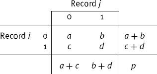
where a denotes the number of predictors for which records i and j do not have that attribute, d is the number of predictors for which the two records have the attribute present, and so on. The most useful similarity measures in this situation are:
Jaquard's Coefficient d/(b +c + d). This coefficient ignores zero matches. This is desirable when we do not want to consider two people to be similar simply because a large number of characteristics are absent in both. For example, if Owns a Corvette is one of the variables, a matching "yes" would be evidence of similarity, but a matching "no" tells us little about whether the two people are similar.
When the measurements are mixed (some continuous and some binary), a similarity coefficient suggested by Gower is very useful. Gowero's similarity measure is a weighted average of the distances computed for each variable, after scaling each variable to a [0,1] scale. It is defined as
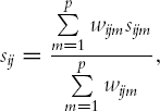
with wijm= 1 subject to the following rules:
wijm= 0 when the value of the measurement is not known for one of the pair of records.
For nonbinary categorical measurements sijm= 0 unless the records are in the same category, in which case sijm= 1.
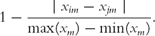
For continuous measurements, sijm=
We define a cluster as a set of one or more records. How do we measure distance between clusters? The idea is to extend measures of distance between records into distances between clusters. Consider cluster A, which includes the m records A1, A2,. . ., Am and cluster B, which includes n records B1, B2,. . ., Bn. The most widely used measures of distance between clusters are:
Minimum Distance (Single Linkage)The distance between the pair of records Ai and Bj that are closest:
min(distance(Ai, Bj)), i = 1, 2,. . ., m;j = 1, 2,. . ., n.
Maximum Distance (Complete Linkage) The distance between the pair of records Ai and Bj that are farthest:
max (distance(Ai, Bj)), i = 1, 2, ..., m; j = 1, 2, ..., n.
Average Distance (Average Linkage) The average distance of all possible distances between records in one cluster and records in the other cluster:
Average(distance(Ai, Bj)), i = 1, 2, ..., m; j = 1, 2, ..., n.
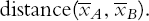
Centroid Distance The distance between the two cluster centroids. A cluster centroid is the vector of measurement averages across all the records in that cluster. For cluster A, this is the vector

Minimum distance, maximum distance, and centroid distance are illustrated visually for two dimensions with a map of Portugal and France in Figure 14.2
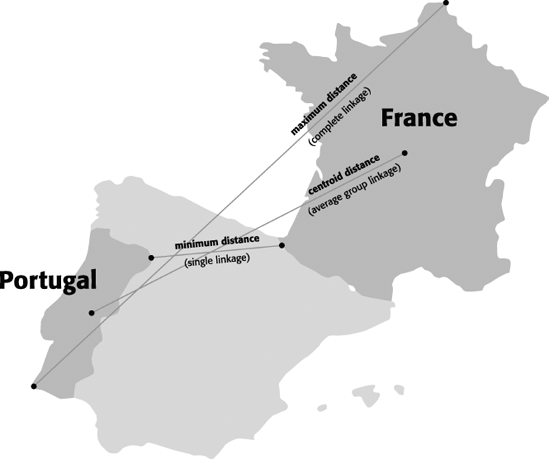
Figure 14.2. TWO-DIMENSIONAL REPRESENTATION OF SEVERAL DIFFERENT DISTANCE MEASURES BETWEEN PORTUGAL AND FRANCE
For instance, consider the first two utilities (Arizona, Boston) as cluster A, and the next three utilities (Central, Commonwealth, Consolidated) as cluster B. Using the normalized scores in Table 14.2 and the distance matrix in Table 14.3, we can compute each of the distances described above. Using Euclidean distance, we get:
The closest pair is Arizona and Commonwealth, and therefore the minimum distance between clusters A and B is 0.76.
The farthest pair is Arizona and Consolidated, and therefore the maximum distance between clusters A and B is 3.02.
The average distance is (0.77 + 0.76 + 3.02 + 1.47 + 1.58 + 1.01)/6 = 1.44.
The centroid of cluster A is
and the centroid of cluster B is
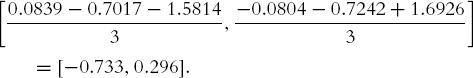
The distance between the two centroids is then
In deciding among clustering methods, domain knowledge is key. If you have good reason to believe that the clusters might be chain- or sausage-like, minimum distance (single linkage) would be a good choice. This method does not require that cluster members all be close to one another, only that the new members being added be close to one of the existing members. An example of an application where this might be the case would be characteristics of crops planted in long rows, or disease outbreaks along navigable waterways that are the main areas of settlement in a region. Another example is laying and finding mines (land or marine). Single linkage is also fairly robust to small deviations in the distances. However, adding or removing data can influence it greatly.
Complete and average linkage are better choices if you know that the clusters are more likely to be spherical (e.g., customers clustered on the basis of numerous attributes). If you do not know the probable nature of the cluster these are good default choices since most clusters tend to be spherical in nature.
We now move to a more detailed description of the two major types of clustering algorithms: hierarchical (agglomerative) and nonhierarchical.
The idea behind hierarchical agglomerative clustering is to start with each cluster comprising exactly one record and then progressively agglomerating (combining) the two nearest clusters until there is just one cluster left at the end, which consists of all the records.
Returning to the small example of five utilities and two measures (Sales and Fuel Cost) and using the distance matrix (Table 14.3), the first step in the hierarchical clustering would join Arizona and Commonwealth, which are the closest (using normalized measurements and Euclidean distance). Next, we would recalculate a 4 × 4 distance matrix that would have the distances between these four clusters: {Arizona,Commonwealth}, {Boston}, {Central}, and {Consolidated}. At this point we use measure of distance between clusters, such as the ones described in the Section 14.3. Each of these distances (minimum, maximum, average, and centroid distance) can be implemented in the hierarchical scheme as described below.
In minimum distance clustering, the distance between two clusters that is used is the minimum distance (the distance between the nearest pair of records in the two clusters, one record in each cluster). In our small utilities example, we would compute the distances between each of {Boston}, {Central}, and {Consolidated} with {Arizona, Commonwealth} to create the 4 × 4 distance matrix shown in Table 14.4.
Table 14.4. DISTANCE MATRIX AFTER ARIZONA AND COMMONWEALTH CONSOLIDATION CLUSTER TOGETHER, USING SINGLE LINKAGE
Arizona-Commonwealth | Boston | Central | Consolidated | |
|---|---|---|---|---|
Arizona-Commonwealth | 0 | |||
Boston | min(2.01,1.58) | 0 | ||
Central | min(0.77,1.02) | 1.47 | 0 | |
Consolidated | min(3.02,2.57) | 1.01 | 2.43 | 0 |
The next step would consolidate {Central} with {Arizona, Commonwealth} because these two clusters are closest. The distance matrix will again be recomputed (this time it will be 3 × 3), and so on.
This method has a tendency to cluster together at an early stage records that are distant from each other because of a chain of intermediate records in the same cluster. Such clusters have elongated sausage-like shapes when visualized as objects in space.
In maximum distance clustering (also called complete linkage) the distance between two clusters is the maximum distance (between the farthest pair of records). If we used complete linkage with the five utilities example, the recomputed distance matrix would be equivalent to Table 14.4, except that the "min" function would be replaced with a "max."
This method tends to produce clusters at the early stages with records that are within a narrow range of distances from each other. If we visualize them as objects in space, the records in such clusters would have roughly spherical shapes.
Average clustering is based on the average distance between clusters (between all possible pairs of records). If we used average linkage with the five utilities example, the recomputed distance matrix would be equivalent to Table 14.4, except that the "min" function would be replaced with an "average."
Note that the results of the single and complete linkage methods depend only on the order of the interrecord distances. Linear transformations of the distances (and other transformations that do not change the order) do not affect the results.
In clustering based on centroid distance (average group linkage clustering), clusters are represented by their mean values for each variable, a vector of means. The distance between two clusters is the distance between these two vectors. In average linkage, above, each pairwise distance is calculated, and the average of all such distances is calculated. In average group linkage or centroid distance clustering, just one distance is calculated, the distance between group means.
Ward's method is also agglomerative in that it joins records and clusters together progressively to produce larger and larger clusters but operates slightly differently from the general approach described above. Ward's method considers the "loss of information" that occurs when record are clustered together. When each cluster has one record, there is no loss of information – all individual values remain available. When records are joined together and represented in clusters, information about an individual record is replaced by the information for the cluster to which it belongs. To measure loss of information, Ward's method employs a measure "error sum of squares" (ESS) that measures the difference between individual observations and a group mean.
This is easiest to see in univariate data. For example, consider the values (2, 6, 5, 6, 2, 2, 2, 2, 0, 0, 0) with a mean of 2.5. Their ESS is equal to (2 − 2.5)2 + (6 − 2.5)2 + (5 − 2.5)2 + ... + (0 − 2.5)2 = 50.5. The loss of information associated with grouping the values into a single group is therefore 50.5. Now group the observations into four groups: (0, 0, 0), (2, 2, 2, 2), (5), and (6, 6). The loss of information is the sum of the ESS's for each group, which is 0 (each observation in each group is equal to the mean for that group, so the ESS for each group is 0). Thus clustering the 10 observations into 4 clusters results in no loss of information, and this would be the first step in Ward's method. In moving to a smaller number of clusters, Ward's method would choose the configuration that results in the smallest incremental loss of information.
Ward's method tends to result in convex clusters that are of roughly equal size, which can be an important consideration in some applications (e.g., in establishing meaningful customer segments).
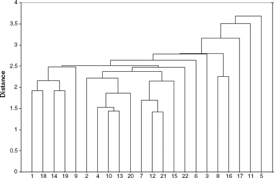
A dendrogram is a treelike diagram that summarizes the process of clustering. At the bottom are the records. Similar records are joined by lines whose vertical length reflects the distance between the records. Figure 14.3 shows the dendrogram that results from clustering all 22 utilities using the 8 normalized measurements, Euclidean distance, and single linkage.
For any given number of clusters, we can determine the records in the clusters by sliding a horizontal line up and down until the number of vertical intersections of the horizontal line equals the number of clusters desired. For example, if we wanted to form six clusters, we would find that the clusters are:
{1, 2, 4, 10, 13, 20, 7,12, 21, 15,14,19, 18, 22, 9, 3},
{8,16} = {Idaho, Puget},
{6} = {Florida},
{17} = {San Diego},
{11} = { Nevada },
{5} = {NY}.
Note that if we wanted five clusters, they would be identical to the six, with the exception that the first two clusters would be merged into one cluster. In general, all hierarchical methods have clusters that are nested within each other as we decrease the number of clusters. This is a valuable property for interpreting clusters and is essential in certain applications, such as taxonomy of varieties of living organisms.
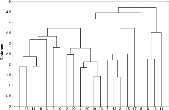
The average linkage dendrogram is shown in Figure 14.4. If we want six clusters using average linkage, they would be
{1, 14, 19, 18, 3,6};{2, 4, 10, 13, 20, 22};{5};{7, 12, 9, 15, 21};{17};{8, 16, 11}.
The goal of cluster analysis is to come up with meaningful clusters. Since there are many variations that can be chosen, it is important to make sure that the resulting clusters are valid, in the sense that they really create some insight.
To see whether the cluster analysis is useful, perform the following:
Cluster Interpretability Is the interpretation of the resulting clusters reasonable? To interpret the clusters, we explore the characteristics of each cluster by
Obtaining summary statistics (e.g., average, min, max) from each cluster on each measurement that was used in the cluster analysis
Examining the clusters for the presence of some common feature (variable) that was not used in the cluster analysis
Cluster labeling: based on the interpretation, trying to assign a name or label to each cluster
Cluster Stability Do cluster assignments change significantly if some of the inputs were altered slightly? Another way to check stability is to partition the data and see how well clusters that are formed based on one part apply to the other part. To do this:
Cluster partition A.
Use the cluster centroids from A to assign each record in partition B (each record is assigned to the cluster with the closest centroid).
Assess how consistent the cluster assignments are compared to the assignments based on all the data.
Cluster Separation Examine the ratio of between-cluster variation to within-cluster variation to see whether the separation is reasonable. There exist statistical tests for this task (an F ratio), but their usefulness is some what controversial.
Returning to the utilities example, we notice that both methods (single and average linkage) identify {5} and {17} as singleton clusters. Also, both dendrograms imply that a reasonable number of clusters in this dataset is four. One insight that can be derived from this clustering is that clusters tend to group geographically:
We can further characterize each of the clusters by examining the summary statistics of their measurements.
Hierarchical clustering is very appealing in that it does not require specification of the number of clusters, and in that sense is purely data driven. The ability to represent the clustering process and results through dendrograms is also an advantage of this method, as it is easier to understand and interpret. There are, however, a few limitations to consider:
Hierarchical clustering requires the computation and storage of an n × n distance matrix. For very large datasets, this can be expensive and slow.
The hierarchical algorithm makes only one pass through the data. This means that records that are allocated incorrectly early in the process cannot be reallocated subsequently.
Hierarchical clustering also tends to have low stability. Reordering data or dropping a few records can lead to a very different solution.
With respect to the choice of distance between clusters, single and complete linkage are robust to changes in the distance metric (e.g., Euclidean, statistical distance) as long as the relative ordering is kept. Average linkage, on the other hand, is much more influenced by the choice of distance metric, and might lead to completely different clusters when the metric is changed.
A nonhierarchical approach to forming good clusters is to prespecify a desired number of clusters, k, and to assign each case to one of k clusters so as to minimize a measure of dispersion within the clusters. In other words, the goal is to divide the sample into a predetermined number k of nonoverlapping clusters so that clusters are as homogeneous as possible with respect to the measurements used.
A very common measure of within-cluster dispersion is the sum of distances (or sum of squared Euclidean distances) of records from their cluster centroid. The problem can be set up as an optimization problem involving integer programming, but because solving integer programs with a large number of variables is time consuming, clusters are often computed using a fast, heuristic method that produces good (although not necessarily optimal) solutions. The k-means algorithm is one such method.
The k-means algorithm starts with an initial partition of the cases into k clusters. Subsequent steps modify the partition to reduce the sum of the distances of each record from its cluster centroid. The modification consists of allocating each record to the nearest of the k centroids of the previous partition. This leads to a new partition for which the sum of distances is smaller than before. The means of the new clusters are computed and the improvement step is repeated until the improvement is very small.
Returning to the example with the five utilities and two measurements, let us assume that k = 2 and that the initial clusters are A = {Arizona, Boston} and B = {Central, Commonwealth, Consolidated}. The cluster centroids were computed in Section 14.4.
The distance of each record from each of these two centroids is shown in Table 14.5. We see that Boston is closer to cluster B, and that Central and Commonwealth are each closer to cluster A. We therefore move each of these records to the other cluster and obtain
A = {Arizona, Central, Commonwealth} and B = {Consolidated, Boston}.
Recalculating the centroids gives
The distance of each record from each of the newly calculated centroids is given in Table 14.6 At this point we stop because each record is allocated to its closest cluster.
The choice of the number of clusters can either be driven by external considerations (e.g., previous knowledge, practical constraints, etc.) or we can try a few different values for k and compare the resulting clusters. After choosing k, the n records are partitioned into these initial clusters. If there is external reasoning that suggests a certain partitioning, this information should be used. Alternatively, if there exists external information on the centroids of the k clusters, this can be used to allocate the records.
In many cases, there is no information to be used for the initial partition. In these cases, the algorithm can be rerun with different randomly generated starting partitions to reduce chances of the heuristic producing a poor solution. The number of clusters in the data is generally not known, so it is a good idea to run the algorithm with different values for k that are near the number of clusters that one expects from the data, to see how the sum of distances reduces with increasing values of k. Note that the clusters obtained using different values of k will not be nested (unlike those obtained by hierarchical methods).
Table 14.6. DISTANCE OF EACH RECORD FROM EACH NEWLY CALCULATED CENTROID
Distance from Centroid A | Distance from Centroid B | |
|---|---|---|
Arizona | 0.3827 | 2.5159 |
Boston | 1.6289 | 0.5067 |
Central | 0.5463 | 1.9432 |
Commonwealth | 0.5391 | 2.0745 |
Consolidated | 2.6412 | 0.5067 |

Figure 14.5. OUTPUT FOR K -MEANS CLUSTERING WITH K = 6 OF 22 UTILITIES (AFTER SORTING BY CLUSTER ID)
The results of running the k-means algorithm for all 22 utilities and 8 measurements with k = 6 are shown in Figure 14.5. As in the results from the hierarchical clustering, we see once again that {5} is a singleton cluster and that some of the previous "geographic" clusters show up here as well.
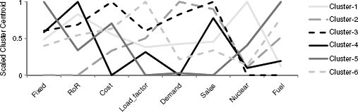
To characterize the resulting clusters, we examine the cluster centroids [numerically in Figure 14.6 or in the line chart ("profile plot") in Figure 14.7]. We can see, for instance, that cluster 1 has the highest average Nuclear, a very high RoR, and a slow demand growth. In contrast, cluster 3 has the highest Sales, with no Nuclear, a high Demand Growth, and the highest average Cost.
We can also inspect the information on the within-cluster dispersion. From Figure 14.6 we see that cluster 2 has the highest average distance, and it includes only two records. In contrast, cluster 1, which includes five records, has the lowest within-cluster average distance. This is true for both normalized measurements (bottom left table) and original units (bottom right table). This means that cluster 1 is more homogeneous.
From the distances between clusters we can learn about the separation of the different clusters. For instance, we see that cluster 2 is very different from the other clusters except cluster 3. This might lead us to examine the possibility of merging the two. Cluster 5, which is a singleton cluster, appears to be very far from all the other clusters.
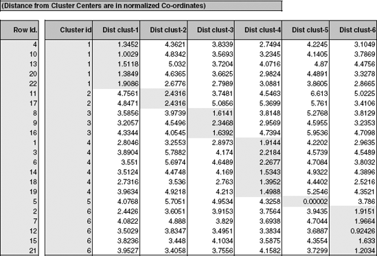
Finally, we can use the information on the distance between the final clusters to evaluate the cluster validity. The ratio of the sum of squared distances for a given k to the sum of squared distances to the mean of all the records (k = 1) is a useful measure for the usefulness of the clustering. If the ratio is near 1.0, the clustering has not been very effective, whereas if it is small, we have well-separated groups.
14.1 University Rankings. The dataset on American College and University Rankings (available from
www.dataminingbook.com) contains information on 1302 American col leges and universities offering an undergraduate program. For each university there are 17 measurements, including continuous measurements (such as tuition and graduation rate) and categorical measurements (such as location by state and whether it is a private or public school).Note that many records are missing some measurements. Our first goal is to estimate these missing values from "similar" records. This will be done by clustering the complete records and then finding the closest cluster for each of the partial records. The missing values will be imputed from the information in that cluster.
Remove all records with missing measurements from the dataset (by creating a new worksheet).
For all the continuous measurements, run hierarchical clustering using complete link age and Euclidean distance. Make sure to normalize the measurements. Examine the dendrogram: How many clusters seem reasonable for describing these data?
Compare the summary statistics for each cluster and describe each cluster in this context (e.g., "Universities with high tuition, low acceptance rate. . ."). Hint: To obtain cluster statistics for hierarchical clustering, use Excel's Pivot Table on the Predicted Clusters sheet.
Use the categorical measurements that were not used in the analysis (State and Private/Public) to characterize the different clusters. Is there any relationship between the clusters and the categorical information?
Can you think of other external information that explains the contents of some or all of these clusters?
Consider Tufts University, which is missing some information. Compute the Eu clidean distance of this record from each of the clusters that you found above (using only the measurements that you have). Which cluster is it closest to? Impute the missing values for Tufts by taking the average of the cluster on those measurements.
14.2 Pharmaceutical Industry. An equities analyst is studying the pharmaceutical industry and would like your help in exploring and understanding the financial data collected by her firm. Her main objective is to understand the structure of the pharmaceutical industry using some basic financial measures.
Financial data gathered on 21 firms in the pharmaceutical industry are available in the file Pharmaceuticals.xls. For each firm, the following variables are recorded:
Use cluster analysis to explore and analyze the given dataset as follows:
Use only the quantitative variables (1-9) to cluster the 21 firms. Justify the various choices made in conducting the cluster analysis, such as weights accorded different variables, the specific clustering algorithm(s) used, the number of clusters formed, and so on.
Interpret the clusters with respect to the quantitative variables that were used in forming the clusters.
Is there a pattern in the clusters with respect to the qualitative variables (10-12) (those not used in forming the clusters)?
Provide an appropriate name for each cluster using any or all of the variables in the dataset.
14.3 Customer Rating of Breakfast Cereals. The dataset Cereals.xls includes nutritional information, store display, and consumer ratings for 77 breakfast cereals.
Data Preprocessing. Remove all cereals with missing values.
Apply hierarchical clustering to the data using Euclidean distance to the standardized measurements. Compare the dendrograms from single linkage and complete linkage, and look at cluster centroids. Comment on the structure of the clusters and on their stability. Hints: (1) To obtain cluster centroids for hierarchical clustering, use Excel's Pivot Table on the Predicted Clusters sheet. (2) Running hierarchical clustering in XLMiner is an iterative process-run it once with a guess at the right number of clusters, then run it again after looking at the dendrogram, adjusting the number of clusters if needed.
Which method leads to the most insightful or meaningful clusters?
Choose one of the methods. How many clusters would you use? What distance is used for this cutoff? (Look at the dendrogram.)
The elementary public schools would like to choose a set of cereals to include in their daily cafeterias. Every day a different cereal is offered, but all cereals should support a healthy diet. For this goal you are requested to find a cluster of "healthy cereals". Should the data be standardized? If not, how should they be used in the cluster analysis?
14.4 Marketing to Frequent Fliers. The file EastWestAirlinesCluster.xls contains information on 4000 passengers who belong to an airline's frequent flier program. For each passenger the data include information on their mileage history and on different ways they accrued or spent miles in the last year. The goal is to try to identify clusters of passengers that have similar characteristics for the purpose of targeting different segments for different types of mileage offers.
Apply hierarchical clustering with Euclidean distance and Ward's method. Make sure to standardize the data first. How many clusters appear?
What would happen if the data were not standardized?
Compare the cluster centroid to characterize the different clusters and try to give each cluster a label.
To check the stability of the clusters, remove a random 5% of the data (by taking a random sample of 95% of the records), and repeat the analysis. Does the same picture emerge?
Use k-means clustering with the number of clusters that you found above. Does the same picture emerge?
Which clusters would you target for offers, and what types of offers would you target to customers in that cluster?