About
This section is included to assist you in performing the activities present in the book. It includes detailed steps that are to be performed by the students to complete and achieve the objectives of the book.
Chapter 1: Introduction to Data Science and Data Preprocessing
Activity 1: Pre-Processing Using the Bank Marketing Subscription Dataset
Solution
Let's perform various pre-processing tasks on the Bank Marketing Subscription dataset. We'll also be splitting the dataset into training and testing data. Follow these steps to complete this activity:
- Open a Jupyter notebook and add a new cell to import the pandas library and load the dataset into a pandas dataframe. To do so, you first need to import the library, and then use the pd.read_csv() function, as shown here:
import pandas as pd
Link = 'https://github.com/TrainingByPackt/Data-Science-with-Python/blob/master/Chapter01/Data/Banking_Marketing.csv'
#reading the data into the dataframe into the object data
df = pd.read_csv(Link, header=0)
- To find the number of rows and columns in the dataset, add the following code:
#Finding number of rows and columns
print("Number of rows and columns : ",df.shape)
The preceding code generates the following output:

Figure 1.60: Number of rows and columns in the dataset
- To print the list of all columns, add the following code:
#Printing all the columns
print(list(df.columns))
The preceding code generates the following output:

Figure 1.61: List of columns present in the dataset
- To overview the basic statistics of each column, such as the count, mean, median, standard deviation, minimum value, maximum value, and so on, add the following code:
#Basic Statistics of each column
df.describe().transpose()
The preceding code generates the following output:
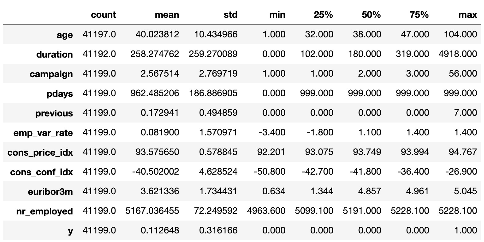
Figure 1.62: Basic statistics of each column
- To print the basic information of each column, add the following code:
#Basic Information of each column
print(df.info())
The preceding code generates the following output:
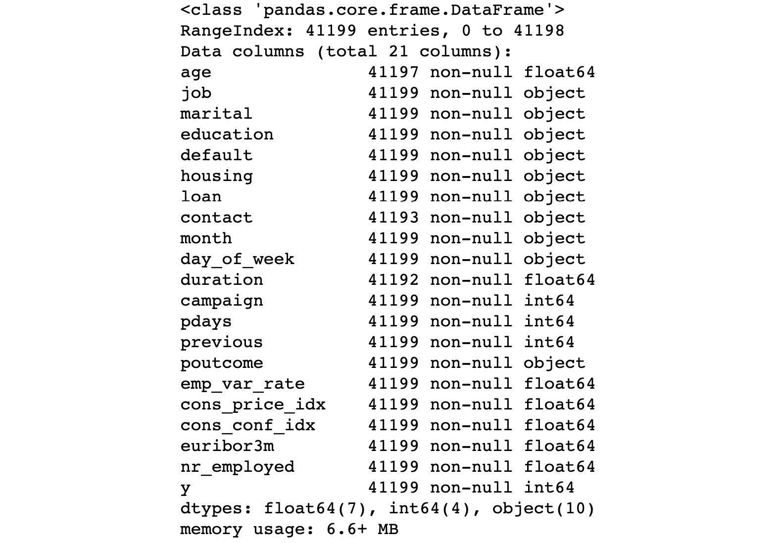
Figure 1.63: Basic information of each column
In the preceding figure, you can see that none of the columns contains any null values. Also, the type of each column is provided.
- Now let's check for missing values and the type of each feature. Add the following code to do this:
#finding the data types of each column and checking for null
null_ = df.isna().any()
dtypes = df.dtypes
sum_na_ = df.isna().sum()
info = pd.concat([null_,sum_na_,dtypes],axis = 1,keys = ['isNullExist','NullSum','type'])
info
Have a look at the output for this in the following figure:
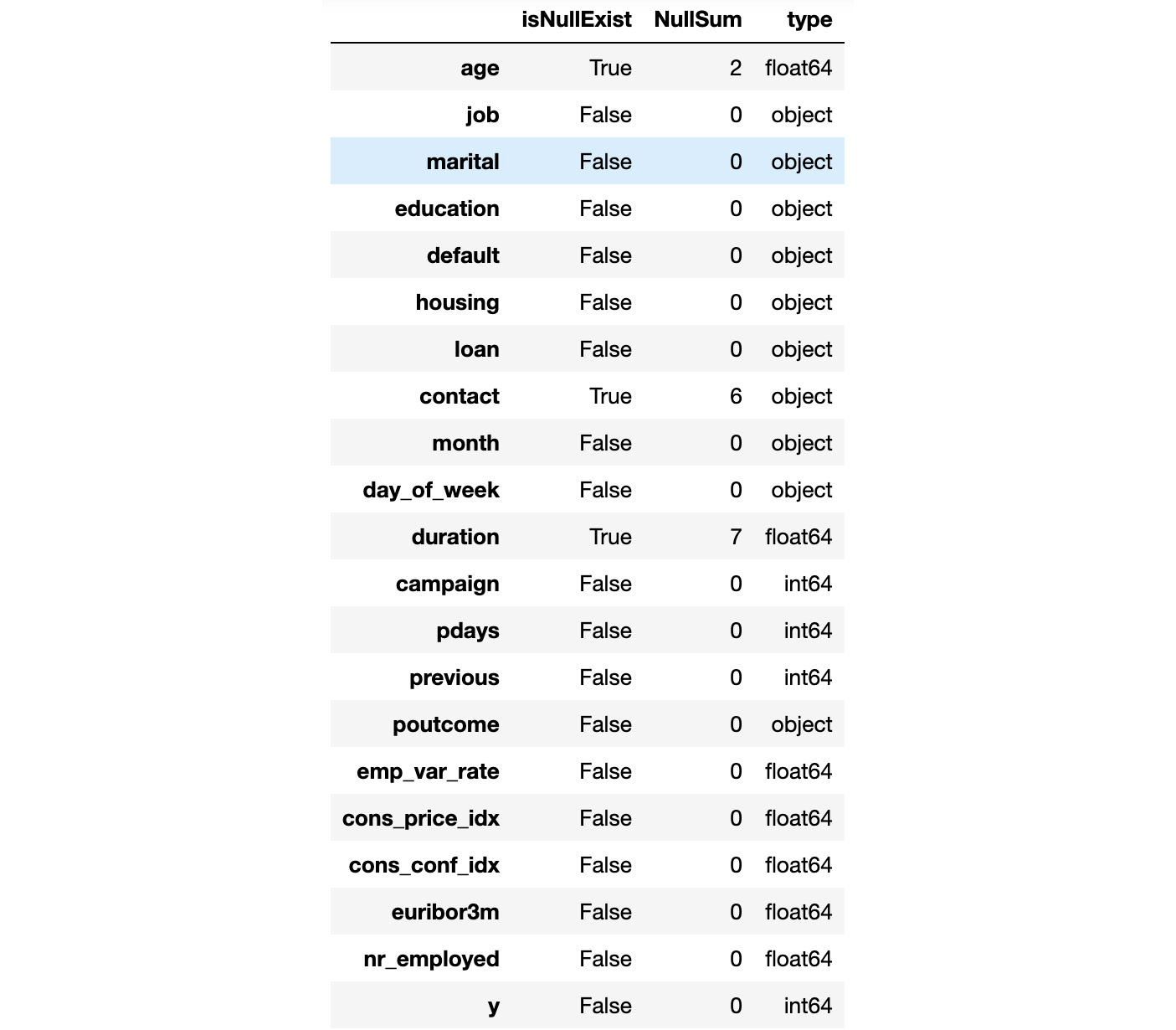
Figure 1.64: Information of each column stating the number of null values and the data types
- Since we have loaded the dataset into the data object, we will remove the null values from the dataset. To remove the null values from the dataset, add the following code:
#removing Null values
df = df.dropna()
#Total number of null in each column
print(df.isna().sum())# No NA
Have a look at the output for this in the following figure:
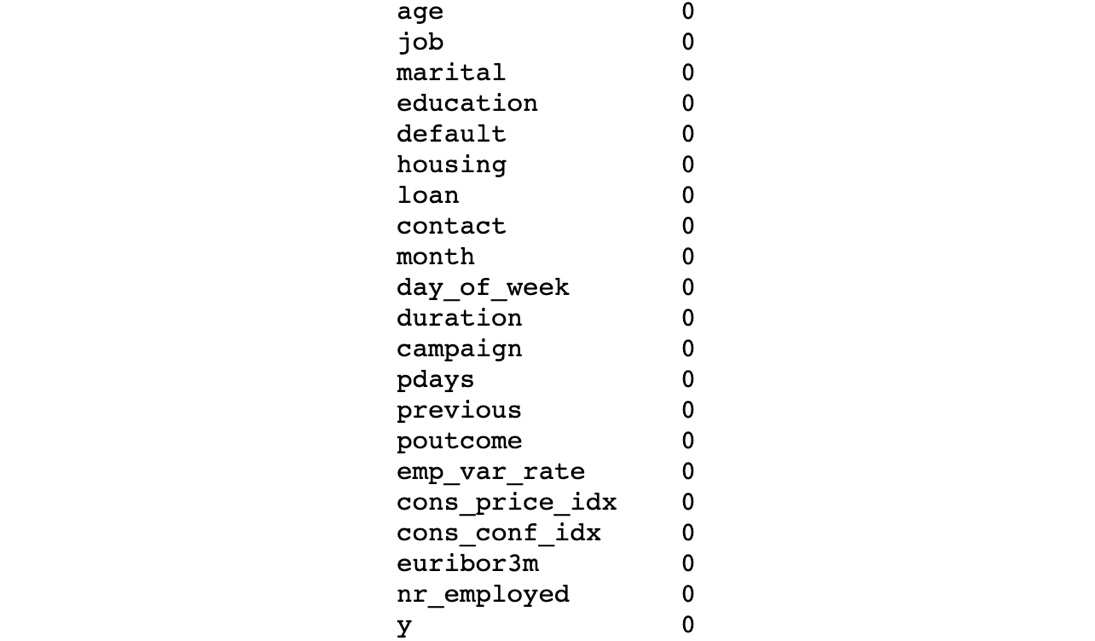
Figure 1.65: Features of dataset with no null values
- Now we check the frequency distribution of the education column in the dataset. Use the value_counts() function to implement this:
df.education.value_counts()
Have a look at the output for this in the following figure:

Figure 1.66: Frequency distribution of the education column
- In the preceding figure, we can see that the education column of the dataset has many categories. We need to reduce the categories for better modeling. To check the various categories in the education column, we use the unique() function. Type the following code to implement this:
df.education.unique()
The output is as follows:
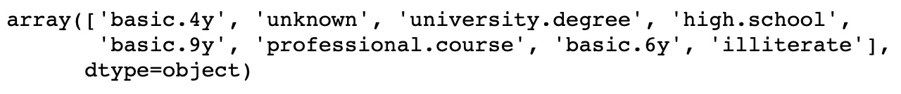
Figure 1.67: Various categories of the education column
- Now let's group the basic.4y, basic.9y, and basic.6y categories together and call them basic. To do this, we can use the replace function from pandas:
df.education.replace({"basic.9y":"Basic","basic.6y":"Basic","basic.4y":"Basic"},inplace=True)
- To check the list of categories after grouping, add the following code:
df.education.unique()

Figure 1.68: Various categories of the education column
In the preceding figure, you can see that basic.9y, basic.6y, and basic.4y are grouped together as Basic.
- Now we select and perform a suitable encoding method for the data. Add the following code to implement this:
#Select all the non numeric data using select_dtypes function
data_column_category = df.select_dtypes(exclude=[np.number]).columns
The preceding code generates the following output:

Figure 1.69: Various columns of the dataset
- Now we define a list with all the names of the categorical features in the data. Also, we loop through every variable in the list, getting dummy variable encoded output. Add the following code to do this:
cat_vars=data_column_category
for var in cat_vars:
cat_list='var'+'_'+var
cat_list = pd.get_dummies(df[var], prefix=var)
data1=df.join(cat_list)
df=data1
df.columns
The preceding code generates the following output:
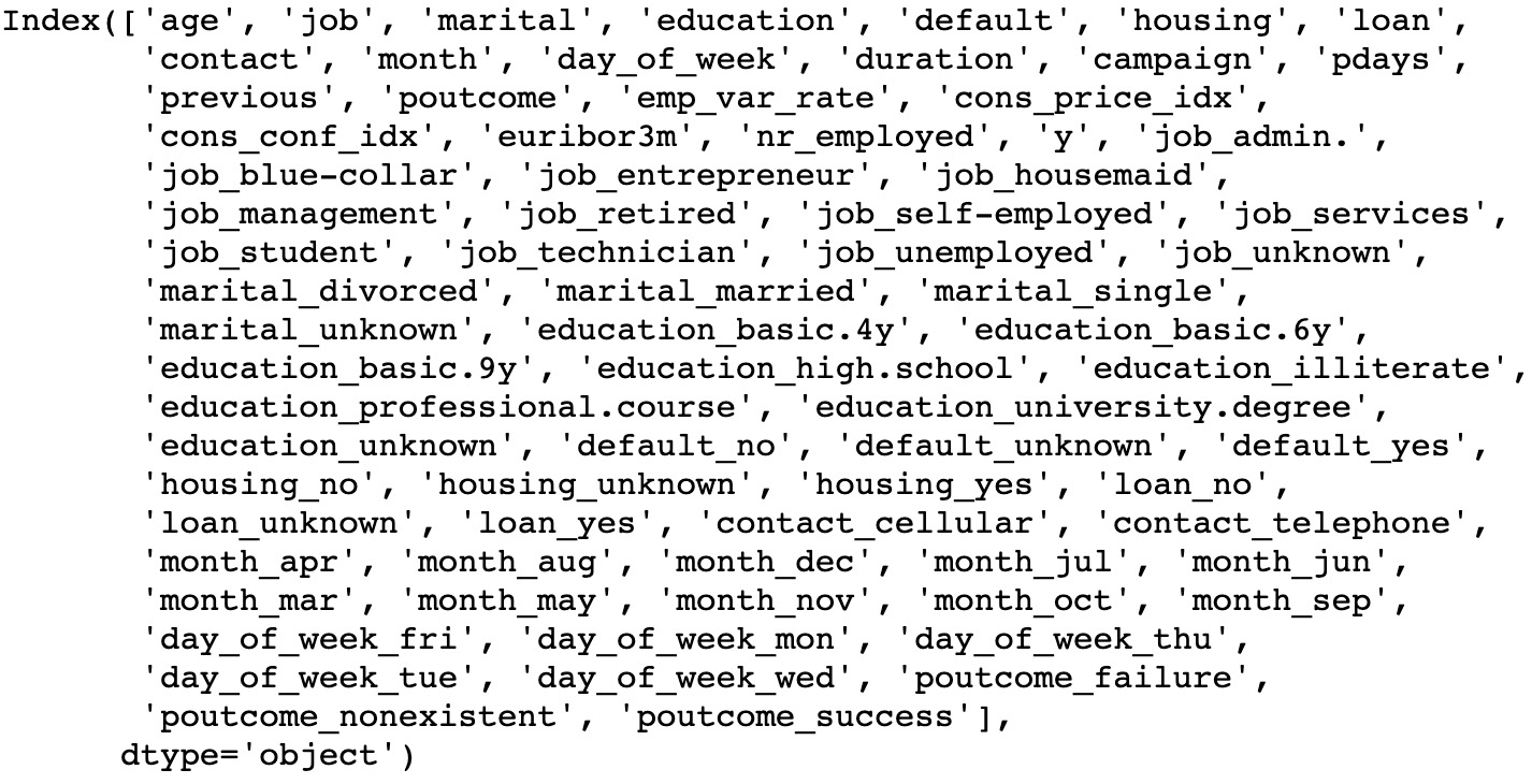
Figure 1.70: List of categorical features in the data
- Now we neglect the categorical column for which we have done encoding. We'll select only the numerical and encoded categorical columns. Add the code to do this:
#Categorical features
cat_vars=data_column_category
#All features
data_vars=df.columns.values.tolist()
#neglecting the categorical column for which we have done encoding
to_keep = []
for i in data_vars:
if i not in cat_vars:
to_keep.append(i)
#selecting only the numerical and encoded catergorical column
data_final=df[to_keep]
data_final.columns
The preceding code generates the following output:
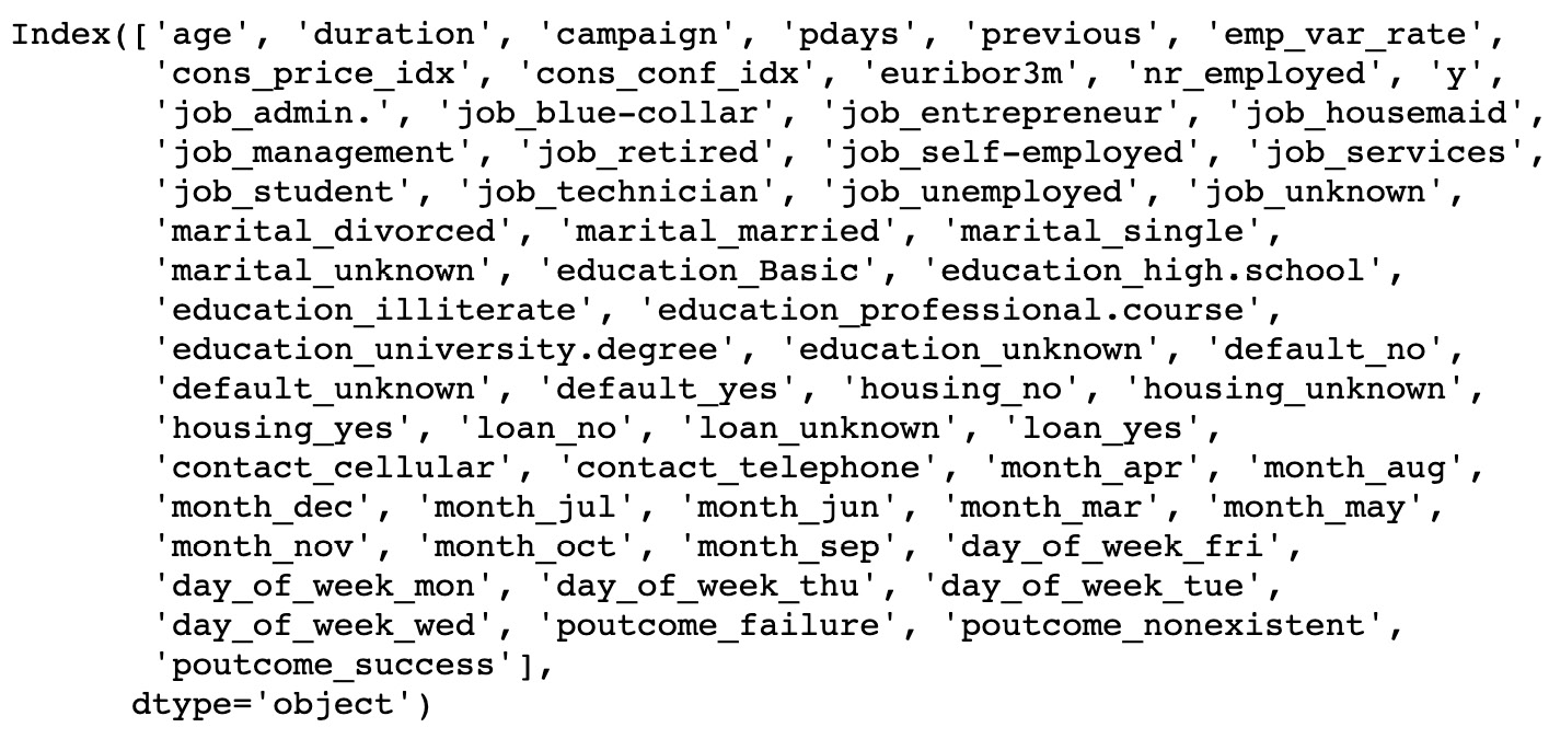
Figure 1.71: List of numerical and encoded categorical columns
- Finally, we split the data into train and test sets. Add the following code to implement this:
#Segregating Independent and Target variable
X=data_final.drop(columns='y')
y=data_final['y']
from sklearn. model_selection import train_test_split
X_train, X_test, y_train, y_test = train_test_split(X, y, test_size=0.2, random_state=0)
print("FULL Dateset X Shape: ", X.shape )
print("Train Dateset X Shape: ", X_train.shape )
print("Test Dateset X Shape: ", X_test.shape )
The output is as follows:

Figure 1.72: Shape of the full, train, and test datasets
Chapter 2: Data Visualization
Activity 2: Line Plot
Solution:
- Create a list of 6 strings for each month, January through June, and save it as x using:
x = ['January','February','March','April','May','June']
- Create a list of 6 values for 'Items Sold' that starts at 1000 and increases by 200, so the final value is 2000 and save it as y as follows:
y = [1000, 1200, 1400, 1600, 1800, 2000]
- Plot y ('Items Sold') by x ('Month') with a dotted blue line and star markers using the following:
plt.plot(x, y, '*:b')
- Set the x-axis to 'Month' using the following code:
plt.xlabel('Month')
- Set the y-axis to 'Items Sold' as follows:
plt.ylabel('Items Sold')
- To set the title to read 'Items Sold has been Increasing Linearly', refer to the following code:
plt.title('Items Sold has been Increasing Linearly')
Check out the following screenshot for the resultant output:
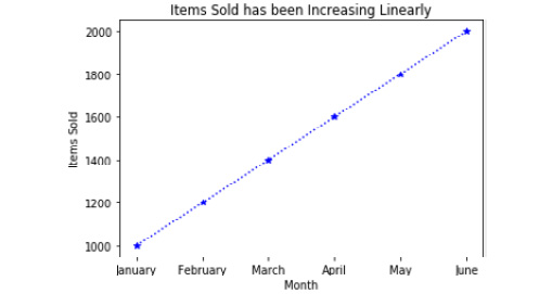
Figure 2.33: Line plot of items sold by month
Activity 3: Bar Plot
Solution:
- Create a list of five strings for x containing the names of NBA franchises with the most titles using the following code:
x = ['Boston Celtics','Los Angeles Lakers', 'Chicago Bulls', 'Golden State Warriors', 'San Antonio Spurs']
- Create a list of five values for y containing values for 'Titles Won' that correspond with the strings in x using the following code:
y = [17, 16, 6, 6, 5]
- Place x and y into a data frame with the column names 'Team' and 'Titles', respectively, as follows:
import pandas as pd
df = pd.DataFrame({'Team': x,
'Titles': y})
- To sort the data frame descending by 'Titles' and save it as df_sorted, refer to the following code:
df_sorted = df.sort_values(by=('Titles'), ascending=False)
Note
If we sort with ascending=True, the plot will have larger values to the right. Since we want the larger values on the left, we will be using ascending=False.
- Make a programmatic title and save it as title by first finding the team with the most titles and saving it as the team_with_most_titles object using the following code:
team_with_most_titles = df_sorted['Team'][0]
- Then, retrieve the number of titles for the team with the most titles using the following code:
most_titles = df_sorted['Titles'][0]
- Lastly, create a string that reads 'The Boston Celtics have the most titles with 17' using the following code:
title = 'The {} have the most titles with {}'.format(team_with_most_titles, most_titles)
- Use a bar graph to plot the number of titles by team using the following code:
import matplotlib.pyplot as plt
plt.bar(df_sorted['Team'], df_sorted['Titles'], color='red')
- Set the x-axis label to 'Team' using the following:
plt.xlabel('Team')
- Set the y-axis label to 'Number of Championships' using the following:
plt.ylabel('Number of Championships')
- To prevent the x tick labels from overlapping by rotating them 45 degrees, refer to the following code:
plt.xticks(rotation=45)
- Set the title of the plot to the programmatic title object we created as follows:
plt.title(title)
- Save the plot to our current working directory as 'Titles_by_Team.png' using the following code:
plt.savefig('Titles_by_Team)
- Print the plot using plt.show(). To understand this better, check out the following output screenshot:
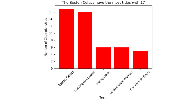
Figure 2.34: The bar plot of the number of titles held by an NBA team
Note
When we print the plot to the console using plt.show(), it appears as intended; however, when we open the file we created titled 'Titles_by_Team.png', we see that it crops the x tick labels.
The following figure displays the bar plot with the cropped x tick labels.
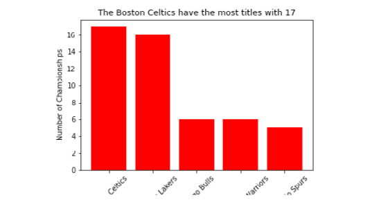
Figure 2.35: 'Titles_by_Team.png' with x tick labels cropped
- To fix the cropping issue, add bbox_inches='tight' as an argument inside of plt.savefig() as follows:
plt.savefig('Titles_by_Team', bbox_inches='tight')
- Now, when we open the saved 'Titles_by_Team.png' file from our working directory, we see that the x tick labels are not cropped.
Check out the following output for the final result:
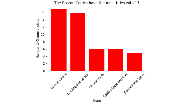
Figure 2.36: 'Titles_by_Team.png' without cropped x tick labels
Activity 4: Multiple Plot Types Using Subplots
Solution:
- Import the 'Items_Sold_by_Week.csv' file and save it as the Items_by_Week data frame object using the following code:
import pandas as pd
Items_by_Week = pd.read_csv('Items_Sold_by_Week.csv')
- Import the 'Weight_by_Height.csv' file and save it as the Weight_by_Height data frame object as follows:
Weight_by_Height = pd.read_csv('Weight_by_Height.csv')
- Generate an array of 100 normally distributed numbers to use as data for the histogram and box-and-whisker plots and save it as y using the following code:
y = np.random.normal(loc=0, scale=0.1, size=100)
- To generate a figure with six subplots organized in three rows and two columns that do not overlap refer to the following code:
import matplotlib.pyplot as plt
fig, axes = plt.subplots(nrows=3, ncols=2)
plt.tight_layout()
- Set the respective axes' titles to match those in Figure 2.32 using the following code:
axes[0,0].set_title('Line')
axes[0,1].set_title('Bar')
axes[1,0].set_title('Horizontal Bar')
axes[1,1].set_title('Histogram')
axes[2,0].set_title('Scatter')
axes[2,1].set_title('Box-and-Whisker')
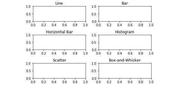
Figure 2.37: Titled, non-overlapping empty subplots
- On the 'Line', 'Bar', and 'Horizontal Bar' axes, plot 'Items_Sold' by 'Week' from 'Items_by_Week' using:
axes[0,0].plot(Items_by_Week['Week'], Items_by_Week['Items_Sold'])
axes[0,1].bar(Items_by_Week['Week'], Items_by_Week['Items_Sold'])
axes[1,0].barh(Items_by_Week['Week'], Items_by_Week['Items_Sold'])
See the resultant output in the following figure:
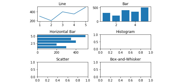
Figure 2.38: Line, bar, and horizontal bar plots added
- On the 'Histogram' and 'Box-and-Whisker' axes, plot the array of 100 normally distributed numbers using the following code:
axes[1,1].hist(y, bins=20)axes[2,1].boxplot(y)
The resultant output is displayed here:
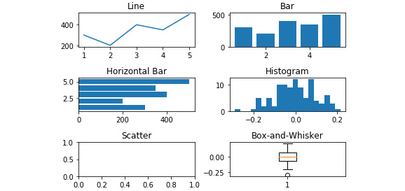
Figure 2.39: The histogram and box-and-whisker added
- Plot 'Weight' by 'Height' on the 'Scatterplot' axes from the 'Weight_by_Height' data frame using the following code:
axes[2,0].scatter(Weight_by_Height['Height'], Weight_by_Height['Weight'])
See the figure here for the resultant output:
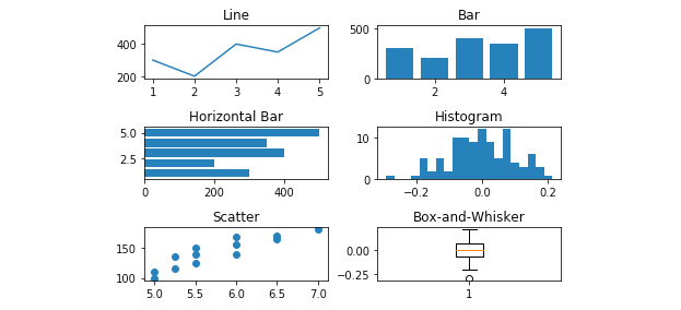
Figure 2.40: Scatterplot added
- Label the x- and y-axis for each subplot using axes[row, column].set_xlabel('X-Axis Label') and axes[row, column].set_ylabel('Y-Axis Label'), respectively.
See the figure here for the resultant output:
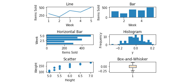
Figure 2.41: X and y axes have been labeled
- Increase the size of the figure with the figsize argument in the subplots function as follows:
fig, axes = plt.subplots(nrows=3, ncols=2, figsize=(8,8))
- Save the figure to the current working directory as 'Six_Subplots' using the following code:
fig.savefig('Six_Subplots')
The following figure displays the 'Six_Subplots.png' file:
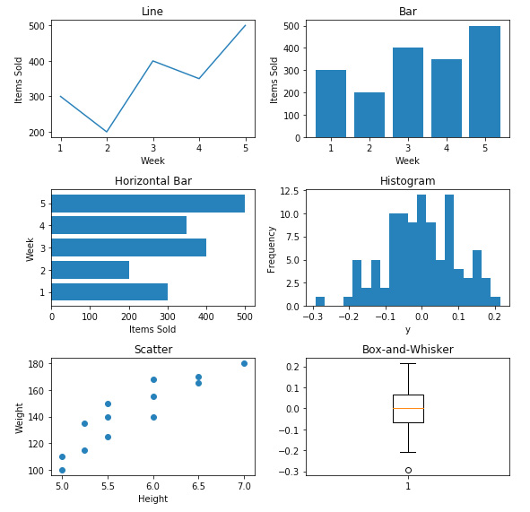
Figure 2.42: The Six_Subplots.png file
Chapter 3: Introduction to Machine Learning via Scikit-Learn
Activity 5: Generating Predictions and Evaluating the Performance of a Multiple Linear Regression Model
Solution:
- Generate predictions on the test data using the following:
predictions = model.predict(X_test)
2. Plot the predicted versus actual values on a scatterplot using the following code:
import matplotlib.pyplot as plt
from scipy.stats import pearsonr
plt.scatter(y_test, predictions)
plt.xlabel('Y Test (True Values)')
plt.ylabel('Predicted Values')
plt.title('Predicted vs. Actual Values (r = {0:0.2f})'.format(pearsonr(y_test, predictions)[0], 2))
plt.show()
Refer to the resultant output here:
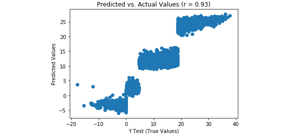
Figure 3.33: A scatterplot of predicted versus actual values from a multiple linear regression model
Note
There is a much stronger linear correlation between the predicted and actual values in the multiple linear regression model (r = 0.93) relative to the simple linear regression model (r = 0.62).
- To plot the distribution of the residuals, refer to the code here:
import seaborn as sns
from scipy.stats import shapiro
sns.distplot((y_test - predictions), bins = 50)
plt.xlabel('Residuals')
plt.ylabel('Density')
plt.title('Histogram of Residuals (Shapiro W p-value = {0:0.3f})'.format(shapiro(y_test - predictions)[1]))
plt.show()
Refer to the resultant output here:
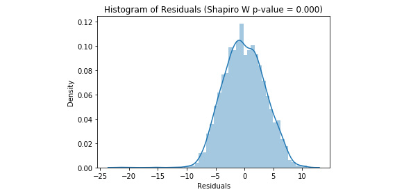
Figure 3.34: The distribution of the residuals from a multiple linear regression model
Note
Our residuals are negatively skewed and non-normal, but this is less skewed than in the simple linear model.
- Calculate the metrics for mean absolute error, mean squared error, root mean squared error, and R-squared, and put them into a DataFrame as follows:
from sklearn import metrics
import numpy as np
metrics_df = pd.DataFrame({'Metric': ['MAE',
'MSE',
'RMSE',
'R-Squared'],
'Value': [metrics.mean_absolute_error(y_test, predictions),
metrics.mean_squared_error(y_test, predictions),
np.sqrt(metrics.mean_squared_error(y_test, predictions)),
metrics.explained_variance_score(y_test, predictions)]}).round(3)
print(metrics_df)
Please refer to the resultant output:

Figure 3.35: Model evaluation metrics from a multiple linear regression model
The multiple linear regression model performed better on every metric relative to the simple linear regression model.
Activity 6: Generating Predictions and Evaluating Performance of a Tuned Logistic Regression Model
Solution:
- Generate the predicted probabilities of rain using the following code:
predicted_prob = model.predict_proba(X_test)[:,1]
- Generate the predicted class of rain using predicted_class = model.predict(X_test).
- Evaluate performance using a confusion matrix and save it as a DataFrame using the following code:
from sklearn.metrics import confusion_matrix
import numpy as np
cm = pd.DataFrame(confusion_matrix(y_test, predicted_class))
cm['Total'] = np.sum(cm, axis=1)
cm = cm.append(np.sum(cm, axis=0), ignore_index=True)
cm.columns = ['Predicted No', 'Predicted Yes', 'Total']
cm = cm.set_index([['Actual No', 'Actual Yes', 'Total']])
print(cm)

Figure 3.36: The confusion matrix from our logistic regression grid search model
Note
Nice! We have decreased our number of false positives from 6 to 2. Additionally, our false negatives were lowered from 10 to 4 (see in Exercise 26). Be aware that results may vary slightly.
- For further evaluation, print a classification report as follows:
from sklearn.metrics import classification_report
print(classification_report(y_test, predicted_class))
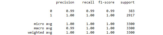
Figure 3.37: The classification report from our logistic regression grid search model
By tuning the hyperparameters of the logistic regression model, we were able to improve upon a logistic regression model that was already performing very well.
Activity 7: Generating Predictions and Evaluating the Performance of the SVC Grid Search Model
Solution:
- Extract predicted classes of rain using the following code:
predicted_class = model.predict(X_test)
- Create and print a confusion matrix using the code here:
from sklearn.metrics import confusion_matrix
import numpy as np
cm = pd.DataFrame(confusion_matrix(y_test, predicted_class))
cm['Total'] = np.sum(cm, axis=1)
cm = cm.append(np.sum(cm, axis=0), ignore_index=True)
cm.columns = ['Predicted No', 'Predicted Yes', 'Total']
cm = cm.set_index([['Actual No', 'Actual Yes', 'Total']])
print(cm)
See the resultant output here:

Figure 3.38: The confusion matrix from our SVC grid search model
- Generate and print a classification report as follows:
from sklearn.metrics import classification_report
print(classification_report(y_test, predicted_class))
See the resultant output here:
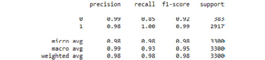
Figure 3.39: The classification report from our SVC grid search model
Here, we demonstrated how to tune the hyperparameters of an SVC model using grid search.
Activity 8: Preparing Data for a Decision Tree Classifier
Solution:
- Import weather.csv and store it as a DataFrame using the following:
import pandas as pd
df = pd.read_csv('weather.csv')
- Dummy code the Description column as follows:
import pandas as pd
df_dummies = pd.get_dummies(df, drop_first=True)
- Shuffle df_dummies using the following code:
from sklearn.utils import shuffle
df_shuffled = shuffle(df_dummies, random_state=42)
- Split df_shuffled into X and y as follows:
DV = 'Rain'
X = df_shuffled.drop(DV, axis=1)
y = df_shuffled[DV]
- Split X and y into testing and training data:
from sklearn.model_selection import train_test_split
X_train, X_test, y_train, y_test = train_test_split(X, y, test_size=0.33, random_state=42)
- Scale X_train and X_test using the following code:
from sklearn.preprocessing import StandardScaler
model = StandardScaler()
X_train_scaled = model.fit_transform(X_train)
X_test_scaled = model.transform(X_test)
Activity 9: Generating Predictions and Evaluating the Performance of a Decision Tree Classifier Model
Solution:
- Generate the predicted probabilities of rain using the following:
predicted_prob = model.predict_proba(X_test_scaled)[:,1]
- Generate the predicted classes of rain using the following:
predicted_class = model.predict(X_test)
- Generate and print a confusion matrix with the code here:
from sklearn.metrics import confusion_matrix
import numpy as np
cm = pd.DataFrame(confusion_matrix(y_test, predicted_class))
cm['Total'] = np.sum(cm, axis=1)
cm = cm.append(np.sum(cm, axis=0), ignore_index=True)
cm.columns = ['Predicted No', 'Predicted Yes', 'Total']
cm = cm.set_index([['Actual No', 'Actual Yes', 'Total']])
print(cm)
Refer to the resultant output here:

Figure 3.40: The confusion matrix from our tuned decision tree classifier model
- Print a classification report as follows:
from sklearn.metrics import classification_report
print(classification_report(y_test, predicted_class))
Refer to the resultant output here:
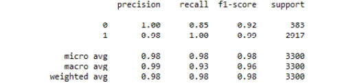
Figure 3.41: The classification report from our tuned decision tree classifier model
There was only one misclassified observation. Thus, by tuning a decision tree classifier model on our weather.csv dataset, we were able to predict rain (or snow) with great accuracy. We can see that the sole driving feature was temperature in Celsius. This makes sense due to the way in which decision trees use recursive partitioning to make predictions.
Activity 10: Tuning a Random Forest Regressor
Solution:
- Specify the hyperparameter space as follows:
import numpy as np
grid = {'criterion': ['mse','mae'],
'max_features': ['auto', 'sqrt', 'log2', None],
'min_impurity_decrease': np.linspace(0.0, 1.0, 10),
'bootstrap': [True, False],
'warm_start': [True, False]}
- Instantiate the GridSearchCV model, optimizing the explained variance using the following code:
from sklearn.model_selection import GridSearchCV
from sklearn.ensemble import RandomForestRegressor
model = GridSearchCV(RandomForestRegressor(), grid, scoring='explained_variance', cv=5)
- Fit the grid search model to the training set using the following (note that this may take a while):
model.fit(X_train_scaled, y_train)
See the output here:
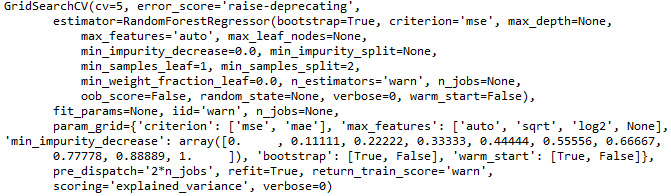
Figure 3.42: The output from our tuned random forest regressor grid search model
- Print the tuned parameters as follows:
best_parameters = model.best_params_
print(best_parameters)
See the resultant output below:
Figure 3.43: The tuned hyperparameters from our random forest regressor grid search model
Activity 11: Generating Predictions and Evaluating the Performance of a Tuned Random Forest Regressor Model
Solution:
- Generate predictions on the test data using the following:
predictions = model.predict(X_test_scaled)
- Plot the correlation of predicted and actual values using the following code:
import matplotlib.pyplot as plt
from scipy.stats import pearsonr
plt.scatter(y_test, predictions)
plt.xlabel('Y Test (True Values)')
plt.ylabel('Predicted Values')
plt.title('Predicted vs. Actual Values (r = {0:0.2f})'.format(pearsonr(y_test, predictions)[0], 2))
plt.show()
Refer to the resultant output here:
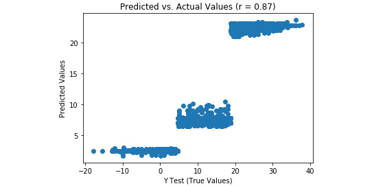
Figure 3.44: A scatterplot of predicted and actual values from our random forest regression model with tuned hyperparameters
- Plot the distribution of residuals as follows:
import seaborn as sns
from scipy.stats import shapiro
sns.distplot((y_test - predictions), bins = 50)
plt.xlabel('Residuals')
plt.ylabel('Density')
plt.title('Histogram of Residuals (Shapiro W p-value = {0:0.3f})'.format(shapiro(y_test - predictions)[1]))
plt.show()
Refer to the resultant output here:
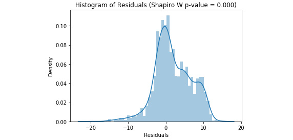
Figure 3.45: A histogram of residuals from a random forest regression model with tuned hyperparameters
- Compute metrics, place them in a DataFrame, and print it using the code here:
from sklearn import metrics
import numpy as np
metrics_df = pd.DataFrame({'Metric': ['MAE',
'MSE',
'RMSE',
'R-Squared'],
'Value': [metrics.mean_absolute_error(y_test, predictions),
metrics.mean_squared_error(y_test, predictions),
np.sqrt(metrics.mean_squared_error(y_test, predictions)),
metrics.explained_variance_score(y_test, predictions)]}).round(3)
print(metrics_df)
Find the resultant output here:

Figure 3.46: Model evaluation metrics from our random forest regression model with tuned hyperparameters
The random forest regressor model seems to underperform compared to the multiple linear regression, as evidenced by greater MAE, MSE, and RMSE values, as well as less explained variance. Additionally, there was a weaker correlation between the predicted and actual values, and the residuals were further from being normally distributed. Nevertheless, by leveraging ensemble methods using a random forest regressor, we constructed a model that explains 75.8% of the variance in temperature and predicts temperature in Celsius + 3.781 degrees.
Chapter 4: Dimensionality Reduction and Unsupervised Learning
Activity 12: Ensemble k-means Clustering and Calculating Predictions
Solution:
After the glass dataset has been imported, shuffled, and standardized (see Exercise 58):
- Instantiate an empty data frame to append each model and save it as the new data frame object labels_df with the following code:
import pandas as pd
labels_df = pd.DataFrame()
- Import the KMeans function outside of the loop using the following:
from sklearn.cluster import KMeans
- Complete 100 iterations as follows:
for i in range(0, 100):
- Save a KMeans model object with two clusters (arbitrarily decided upon, a priori) using:
model = KMeans(n_clusters=2)
- Fit the model to scaled_features using the following:
model.fit(scaled_features)
- Generate the labels array and save it as the labels object, as follows:
labels = model.labels_
- Store labels as a column in labels_df named after the iteration using the code:
labels_df['Model_{}_Labels'.format(i+1)] = labels
- After labels have been generated for each of the 100 models (see Activity 21), calculate the mode for each row using the following code:
row_mode = labels_df.mode(axis=1)
- Assign row_mode to a new column in labels_df, as shown in the following code:
labels_df['row_mode'] = row_mode
- View the first five rows of labels_df
print(labels_df.head(5))

Figure 4.24: First five rows of labels_df
We have drastically increased the confidence in our predictions by iterating through numerous models, saving the predictions at each iteration, and assigning the final predictions as the mode of these predictions. However, these predictions were generated by models using a predetermined number of clusters. Unless we know the number of clusters a priori, we will want to discover the optimal number of clusters to segment our observations.
Activity 13: Evaluating Mean Inertia by Cluster after PCA Transformation
Solution:
- Instantiate a PCA model with the value for the n_components argument equal to best_n_components (that is, remember, best_n_components = 6) as follows:
from sklearn.decomposition import PCA
model = PCA(n_components=best_n_components)
- Fit the model to scaled_features and transform them into the six components, as shown here:
df_pca = model.fit_transform(scaled_features)
- Import numpy and the KMeans function outside the loop using the following code:
from sklearn.cluster import KMeans
import numpy as np
- Instantiate an empty list, inertia_list, for which we will append inertia values after each iteration using the following code:
inertia_list = []
- In the inside for loop, we will iterate through 100 models as follows:
for i in range(100):
- Build our KMeans model with n_clusters=x using:
model = KMeans(n_clusters=x)
Note
The value for x will be dictated by the outer loop which is covered in detail here.
- Fit the model to df_pca as follows:
model.fit(df_pca)
- Get the inertia value and save it to the object inertia using the following code:
inertia = model.inertia_
- Append inertia to inertia_list using the following code:
inertia_list.append(inertia)
- Moving to the outside loop, instantiate another empty list to store the average inertia values using the following code:
mean_inertia_list_PCA = []
- Since we want to check the average inertia over 100 models for n_clusters 1 through 10, we will instantiate the outer loop as follows:
for x in range(1, 11):
- After the inside loop has run through its 100 iterations, and the inertia value for each of the 100 models have been appended to inertia_list, compute the mean of this list, and save the object as mean_inertia using the following code:
mean_inertia = np.mean(inertia_list)
- Append mean_inertia to mean_inertia_list_PCA using the following code:
mean_inertia_list_PCA.append(mean_inertia)
- Print mean_inertia_list_PCA to the console using the following code:
print(mean_inertia_list_PCA)
- Notice the output in the following screenshot:
Figure 4.25: mean_inertia_list_PCA
Chapter 5: Mastering Structured Data
Activity 14: Training and Predicting the Income of a Person
Solution:
- Import the libraries and load the income dataset using pandas. First, import pandas and then read the data using read_csv.
import pandas as pd
import xgboost as xgb
import numpy as np
from sklearn.metrics import accuracy_score
data = pd.read_csv("../data/adult-data.csv", names=['age', 'workclass', 'education-num', 'occupation', 'capital-gain', 'capital-loss', 'hours-per-week', 'income'])
The reason we are passing the names of the columns is because the data doesn't contain them. We do this to make our lives easy.
- Use Label Encoder from sklearn to encode strings. First, import Label Encoder. Then, encode all string categorical columns one by one.
from sklearn.preprocessing import LabelEncoder
data['workclass'] = LabelEncoder().fit_transform(data['workclass'])
data['occupation'] = LabelEncoder().fit_transform(data['occupation'])
data['income'] = LabelEncoder().fit_transform(data['income'])
Here, we encode all the categorical string data that we have. There is another method we can use to prevent writing the same piece of code again and again. See if you can find it.
- We first separate the dependent and independent variables.
X = data.copy()
X.drop("income", inplace = True, axis = 1)
Y = data.income
- Then, we divide them into training and testing sets with an 80:20 split.
X_train, X_test = X[:int(X.shape[0]*0.8)].values, X[int(X.shape[0]*0.8):].values
Y_train, Y_test = Y[:int(Y.shape[0]*0.8)].values, Y[int(Y.shape[0]*0.8):].values
- Next, we convert them into DMatrix, a data structure that the library supports.
train = xgb.DMatrix(X_train, label=Y_train)
test = xgb.DMatrix(X_test, label=Y_test)
- Then, we use the following parameters to train the model using XGBoost.
param = {'max_depth':7, 'eta':0.1, 'silent':1, 'objective':'binary:hinge'} num_round = 50
model = xgb.train(param, train, num_round)
- Check the accuracy of the model.
preds = model.predict(test)
accuracy = accuracy_score(Y[int(Y.shape[0]*0.8):].values, preds)
print("Accuracy: %.2f%%" % (accuracy * 100.0))
The output is as follows:
Figure 5.36: Final model accuracy
Activity 15: Predicting the Loss of Customers
Solution:
- Load the income dataset using pandas. First, import pandas, and then read the data using read_csv.
import pandas as pd
import numpy as np
data = data = pd.read_csv("data/telco-churn.csv")
- The customerID variable is not required because any future prediction will have a unique customerID, making this variable useless for prediction.
data.drop('customerID', axis = 1, inplace = True)
- Convert all categorical variables to integers using scikit. One example is given below.
from sklearn.preprocessing import LabelEncoder
data['gender'] = LabelEncoder().fit_transform(data['gender'])
- Check the data types of the variables in the dataset.
data.dtypes
The data types of the variables will be shown as follows:
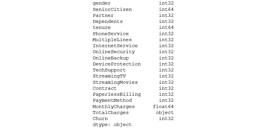
Figure 5.37: Data types of variables
- As you can see, TotalCharges is an object. So, convert the data type of TotalCharges from object to numeric. coerce will make the missing values null.
data.TotalCharges = pd.to_numeric(data.TotalCharges, errors='coerce')
- Convert the data frame to an XGBoost variable and find the best parameters for the dataset using the previous exercises as reference.
import xgboost as xgb
import matplotlib.pyplot as plt
X = data.copy()
X.drop("Churn", inplace = True, axis = 1)
Y = data.Churn
X_train, X_test = X[:int(X.shape[0]*0.8)].values, X[int(X.shape[0]*0.8):].values
Y_train, Y_test = Y[:int(Y.shape[0]*0.8)].values, Y[int(Y.shape[0]*0.8):].values
train = xgb.DMatrix(X_train, label=Y_train)
test = xgb.DMatrix(X_test, label=Y_test)
test_error = {}
for i in range(20):
param = {'max_depth':i, 'eta':0.1, 'silent':1, 'objective':'binary:hinge'}
num_round = 50
model_metrics = xgb.cv(param, train, num_round, nfold = 10)
test_error[i] = model_metrics.iloc[-1]['test-error-mean']
plt.scatter(test_error.keys(),test_error.values())
plt.xlabel('Max Depth')
plt.ylabel('Test Error')
plt.show()
Check out the output in the following screenshot:
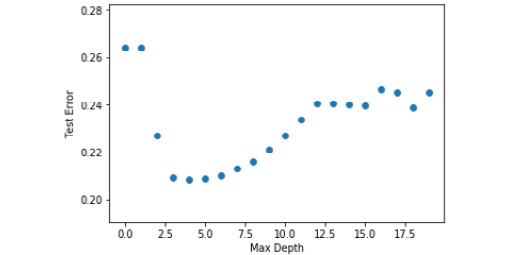
Figure 5.38: Graph of max depth to test error for telecom churn dataset
From the graph, it is clear that a max depth of 4 gives the least error. So, we will be using that to train our model.
- Create the model using the max_depth parameter that we chose from the previous steps.
param = {'max_depth':4, 'eta':0.1, 'silent':1, 'objective':'binary:hinge'}
num_round = 100
model = xgb.train(param, train, num_round)
preds = model.predict(test)
from sklearn.metrics import accuracy_score
accuracy = accuracy_score(Y[int(Y.shape[0]*0.8):].values, preds)
print("Accuracy: %.2f%%" % (accuracy * 100.0))
The output is as follows:

Figure 5.39: Final accuracy
- Save the model for future use using the following code:
model.save_model('churn-model.model')
Activity 16: Predicting a Customer's Purchase Amount
Solution:
- Load the Black Friday dataset using pandas. First, import pandas, and then, read the data using read_csv.
import pandas as pd
import numpy as np
data = data = pd.read_csv("data/BlackFriday.csv")
- The User_ID variable is not required to allow predictions on new user Ids, so we drop it.
data.isnull().sum()
data.drop(['User_ID', 'Product_Category_2', 'Product_Category_3'], axis = 1, inplace = True)
The product category variables have high null values, so we drop them as well.
- Convert all categorical variables to integers using scikit-learn.
from collections import defaultdict
from sklearn.preprocessing import LabelEncoder, MinMaxScaler
label_dict = defaultdict(LabelEncoder)
data[['Product_ID', 'Gender', 'Age', 'Occupation', 'City_Category', 'Stay_In_Current_City_Years', 'Marital_Status', 'Product_Category_1']] = data[['Product_ID', 'Gender', 'Age', 'Occupation', 'City_Category', 'Stay_In_Current_City_Years', 'Marital_Status', 'Product_Category_1']].apply(lambda x: label_dict[x.name].fit_transform(x))
- Split the data into training and testing sets and convert it into the form required by the embedding layers.
from sklearn.model_selection import train_test_split
X = data
y = X.pop('Purchase')
X_train, X_test, y_train, y_test = train_test_split(X, y, test_size=0.3, random_state=9)
cat_cols_dict = {col: list(data[col].unique()) for col in ['Product_ID', 'Gender', 'Age', 'Occupation', 'City_Category', 'Stay_In_Current_City_Years', 'Marital_Status', 'Product_Category_1']}
train_input_list = []
test_input_list = []
for col in cat_cols_dict.keys():
raw_values = np.unique(data[col])
value_map = {}
for i in range(len(raw_values)):
value_map[raw_values[i]] = i
train_input_list.append(X_train[col].map(value_map).values)
test_input_list.append(X_test[col].map(value_map).fillna(0).values)
- Create the network using the embedding and dense layers in Keras and perform hyperparameter tuning to get the best accuracy.
from keras.models import Model
from keras.layers import Input, Dense, Concatenate, Reshape, Dropout
from keras.layers.embeddings import Embedding
cols_out_dict = {
'Product_ID': 20,
'Gender': 1,
'Age': 2,
'Occupation': 6,
'City_Category': 1,
'Stay_In_Current_City_Years': 2,
'Marital_Status': 1,
'Product_Category_1': 9
}
inputs = []
embeddings = []
for col in cat_cols_dict.keys():
inp = Input(shape=(1,), name = 'input_' + col)
embedding = Embedding(len(cat_cols_dict[col]), cols_out_dict[col], input_length=1, name = 'embedding_' + col)(inp)
embedding = Reshape(target_shape=(cols_out_dict[col],))(embedding)
inputs.append(inp)
embeddings.append(embedding)
- Now, we create a three-layer network after the embedding layers.
x = Concatenate()(embeddings)
x = Dense(4, activation='relu')(x)
x = Dense(2, activation='relu')(x)
output = Dense(1, activation='relu')(x)
model = Model(inputs, output)
model.compile(loss='mae', optimizer='adam')
model.fit(train_input_list, y_train, validation_data = (test_input_list, y_test), epochs=20, batch_size=128)
- Check the RMSE of the model on the test set.
from sklearn.metrics import mean_squared_error
y_pred = model.predict(test_input_list)
np.sqrt(mean_squared_error(y_test, y_pred))
The RMSE is:

Figure 5.40: RMSE model
- Visualize the product ID embedding.
import matplotlib.pyplot as plt
from sklearn.decomposition import PCA
embedding_Product_ID = model.get_layer('embedding_Product_ID').get_weights()[0]
pca = PCA(n_components=2)
Y = pca.fit_transform(embedding_Product_ID[:40])
plt.figure(figsize=(8,8))
plt.scatter(-Y[:, 0], -Y[:, 1])
for i, txt in enumerate(label_dict['Product_ID'].inverse_transform(cat_cols_dict['Product_ID'])[:40]):
plt.annotate(txt, (-Y[i, 0],-Y[i, 1]), xytext = (-20, 8), textcoords = 'offset points')
plt.show()
The plot is as follows:

Figure 5.41: Plot of clustered model
From the plot, you can see that similar products have been clustered together by the model.
- Save the model for future use.
model.save ('black-friday.model')
Chapter 6: Decoding Images
Activity 17: Predict if an Image Is of a Cat or a Dog
Solution:
- If you look at the name of the images in the dataset, you will find that the images of dogs start with dog followed by '.' and then a number, for example – "dog.123.jpg". Similarly, the images of cats start with cat. So, let's create a function to get the label from the name of the file:
def get_label(file):
class_label = file.split('.')[0]
if class_label == 'dog': label_vector = [1,0]
elif class_label == 'cat': label_vector = [0,1]
return label_vector
Then, create a function to read, resize, and preprocess the images:
import os
import numpy as np
from PIL import Image
from tqdm import tqdm
from random import shuffle
SIZE = 50
def get_data():
data = []
files = os.listdir(PATH)
for image in tqdm(files):
label_vector = get_label(image)
img = Image.open(PATH + image).convert('L')
img = img.resize((SIZE,SIZE))
data.append([np.asarray(img),np.array(label_vector)])
shuffle(data)
return data
SIZE here refers to the dimension of the final square image we will input to the model. We resize the image to have the length and breadth equal to SIZE.
Note
When running os.listdir(PATH), you will find that all the images of cats come first, followed by images of dogs.
- To have the same distribution of both the classes in the training and testing sets, we will shuffle the data.
- Define the size of the image and read the data. Split the loaded data into training and testing sets:
data = get_data()
train = data[:7000]
test = data[7000:]
x_train = [data[0] for data in train]
y_train = [data[1] for data in train]
x_test = [data[0] for data in test]
y_test = [data[1] for data in test]
- Transform the lists to numpy arrays and reshape the images to a format that Keras will accept:
y_train = np.array(y_train)
y_test = np.array(y_test)
x_train = np.array(x_train).reshape(-1, SIZE, SIZE, 1)
x_test = np.array(x_test).reshape(-1, SIZE, SIZE, 1)
- Create a CNN model that makes use of regularization to perform training:
from keras.models import Sequential
from keras.layers import Dense, Dropout, Conv2D, MaxPool2D, Flatten, BatchNormalization
model = Sequential()
Add the convolutional layers:
model.add(Conv2D(48, (3, 3), activation='relu', padding='same', input_shape=(50,50,1)))
model.add(Conv2D(48, (3, 3), activation='relu'))
Add the pooling layer:
model.add(MaxPool2D(pool_size=(2, 2)))
- Add the batch normalization layer along with a dropout layer using the following code:
model.add(BatchNormalization())
model.add(Dropout(0.10))
- Flatten the 2D matrices into 1D vectors:
model.add(Flatten())
- Use dense layers as the final layers for the model:
model.add(Dense(512, activation='relu'))
model.add(Dropout(0.5))
model.add(Dense(2, activation='softmax'))
- Compile the model and then train it using the training data:
model.compile(loss='categorical_crossentropy',
optimizer='adam',
metrics = ['accuracy'])
Define the number of epochs you want to train the model for:
EPOCHS = 10
model_details = model.fit(x_train, y_train,
batch_size = 128,
epochs = EPOCHS,
validation_data= (x_test, y_test),
verbose=1)
- Print the model's accuracy on the test set:
score = model.evaluate(x_test, y_test)
print("Accuracy: {0:.2f}%".format(score[1]*100))

Figure 6.39: Model accuracy on the test set
- Print the model's accuracy on the training set:
score = model.evaluate(x_train, y_train)
print("Accuracy: {0:.2f}%".format(score[1]*100))
Figure 6.40: Model accuracy on the train set
The test set accuracy for this model is 70.4%. The training set accuracy is really high, at 96%. This means that the model has started to overfit. Improving the model to get the best possible accuracy is left for you as an exercise. You can plot the incorrectly predicted images using the code from previous exercises to get a sense of how well the model performs:
import matplotlib.pyplot as plt
y_pred = model.predict(x_test)
incorrect_indices = np.nonzero(np.argmax(y_pred,axis=1) != np.argmax(y_test,axis=1))[0]
labels = ['dog', 'cat']
image = 5
plt.imshow(x_test[incorrect_indices[image]].reshape(50,50), cmap=plt.get_cmap('gray'))
plt.show()
print("Prediction: {0}".format(labels[np.argmax(y_pred[incorrect_indices[image]])]))
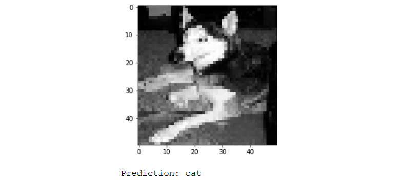
Figure 6.41: Incorrect prediction of a dog by the regularized CNN model
Activity 18: Identifying and Augmenting an Image
Solution:
- Create functions to get the images and the labels of the dataset:
from PIL import Image
def get_input(file):
return Image.open(PATH+file)
def get_output(file):
class_label = file.split('.')[0]
if class_label == 'dog': label_vector = [1,0]
elif class_label == 'cat': label_vector = [0,1]
return label_vector
- Create functions to preprocess and augment images:
SIZE = 50
def preprocess_input(image):
# Data preprocessing
image = image.convert('L')
image = image.resize((SIZE,SIZE))
# Data augmentation
random_vertical_shift(image, shift=0.2)
random_horizontal_shift(image, shift=0.2)
random_rotate(image, rot_range=45)
random_horizontal_flip(image)
return np.array(image).reshape(SIZE,SIZE,1)
- Implement the augmentation functions to randomly execute the augmentation when passed an image and return the image with the result.
This is for horizontal flip:
import random
def random_horizontal_flip(image):
toss = random.randint(1, 2)
if toss == 1:
return image.transpose(Image.FLIP_LEFT_RIGHT)
else:
return image
This is for rotation:
def random_rotate(image, rot_range):
value = random.randint(-rot_range,rot_range)
return image.rotate(value)
This is for image shift:
import PIL
def random_horizontal_shift(image, shift):
width, height = image.size
rand_shift = random.randint(0,shift*width)
image = PIL.ImageChops.offset(image, rand_shift, 0)
image.paste((0), (0, 0, rand_shift, height))
return image
def random_vertical_shift(image, shift):
width, height = image.size
rand_shift = random.randint(0,shift*height)
image = PIL.ImageChops.offset(image, 0, rand_shift)
image.paste((0), (0, 0, width, rand_shift))
return image
- Finally, create the generator that will generate images batches to be used to train the model:
import numpy as np
def custom_image_generator(images, batch_size = 128):
while True:
# Randomly select images for the batch
batch_images = np.random.choice(images, size = batch_size)
batch_input = []
batch_output = []
# Read image, perform preprocessing and get labels
for file in batch_images:
# Function that reads and returns the image
input_image = get_input(file)
# Function that gets the label of the image
label = get_output(file)
# Function that pre-processes and augments the image
image = preprocess_input(input_image)
batch_input.append(image)
batch_output.append(label)
batch_x = np.array(batch_input)
batch_y = np.array(batch_output)
# Return a tuple of (images,labels) to feed the network
yield(batch_x, batch_y)
- Create functions to load the test dataset's images and labels:
def get_label(file):
class_label = file.split('.')[0]
if class_label == 'dog': label_vector = [1,0]
elif class_label == 'cat': label_vector = [0,1]
return label_vector
This get_data function is similar to the one we used in Activity 1. The modification here is that we get the list of images to be read as an input parameter, and we return a tuple of images and their labels:
def get_data(files):
data_image = []
labels = []
for image in tqdm(files):
label_vector = get_label(image)
img = Image.open(PATH + image).convert('L')
img = img.resize((SIZE,SIZE))
labels.append(label_vector)
data_image.append(np.asarray(img).reshape(SIZE,SIZE,1))
data_x = np.array(data_image)
data_y = np.array(labels)
return (data_x, data_y)
- Now, create the test train split and load the test dataset:
import os
files = os.listdir(PATH)
random.shuffle(files)
train = files[:7000]
test = files[7000:]
validation_data = get_data(test)
- Create the model and perform training:
from keras.models import Sequential
model = Sequential()
Add the convolutional layers
from keras.layers import Input, Dense, Dropout, Conv2D, MaxPool2D, Flatten, BatchNormalization
model.add(Conv2D(32, (3, 3), activation='relu', padding='same', input_shape=(50,50,1)))
model.add(Conv2D(32, (3, 3), activation='relu'))
Add the pooling layer:
model.add(MaxPool2D(pool_size=(2, 2)))
- Add the batch normalization layer along with a dropout layer:
model.add(BatchNormalization())
model.add(Dropout(0.10))
- Flatten the 2D matrices into 1D vectors:
model.add(Flatten())
- Use dense layers as the final layers for the model:
model.add(Dense(512, activation='relu'))
model.add(Dropout(0.5))
model.add(Dense(2, activation='softmax'))
- Compile the model and train it using the generator that you created:
EPOCHS = 10
BATCH_SIZE = 128
model.compile(loss='categorical_crossentropy',
optimizer='adam',
metrics = ['accuracy'])
model_details = model.fit_generator(custom_image_generator(train, batch_size = BATCH_SIZE),
steps_per_epoch = len(train) // BATCH_SIZE,
epochs = EPOCHS,
validation_data= validation_data,
verbose=1)
The test set accuracy for this model is 72.6%, which is an improvement on the model in Activity 21. You will observe that the training accuracy is really high, at 98%. This means that this model has started to overfit, much like the one in Activity 21. This could be due to a lack of data augmentation. Try changing the data augmentation parameters to see if there is any change in accuracy. Alternatively, you can modify the architecture of the neural network to get better results. You can plot the incorrectly predicted images to get a sense of how well the model performs.
import matplotlib.pyplot as plt
y_pred = model.predict(validation_data[0])
incorrect_indices = np.nonzero(np.argmax(y_pred,axis=1) != np.argmax(validation_data[1],axis=1))[0]
labels = ['dog', 'cat']
image = 7
plt.imshow(validation_data[0][incorrect_indices[image]].reshape(50,50), cmap=plt.get_cmap('gray'))
plt.show()
print("Prediction: {0}".format(labels[np.argmax(y_pred[incorrect_indices[image]])]))
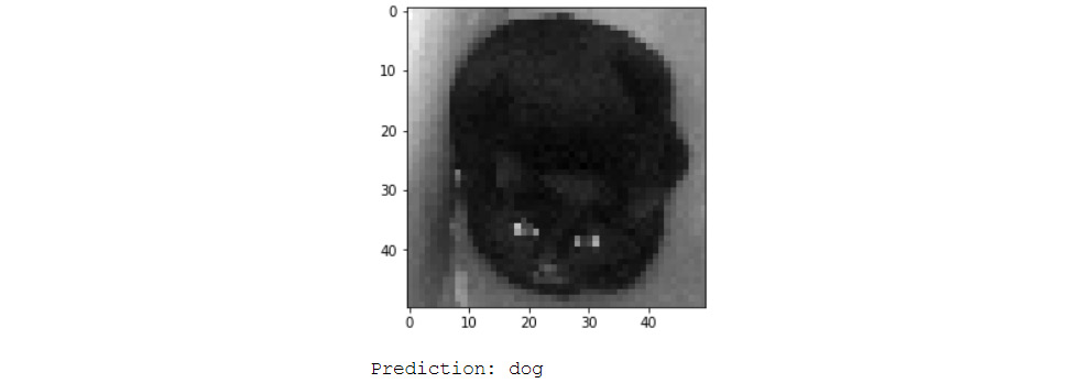
Figure 6.42: Incorrect prediction of a cat by the data augmentation CNN model
Chapter 7: Processing Human Language
Activity 19: Predicting Sentiments of Movie Reviews
Solution:
- Read the IMDB movie review dataset using pandas in Python:
import pandas as pd
data = pd.read_csv('../../chapter 7/data/movie_reviews.csv', encoding='latin-1')
- Convert the tweets to lowercase to reduce the number of unique words:
data.text = data.text.str.lower()
Note
Keep in mind that "Hello" and "hellow" are not the same to a computer.
- Clean the reviews using RegEx with the clean_str function:
import re
def clean_str(string):
string = re.sub(r"https?://S+", '', string)
string = re.sub(r'<a href', ' ', string)
string = re.sub(r'&', '', string)
string = re.sub(r'<br />', ' ', string)
string = re.sub(r'[_"-;%()|+&=*%.,!?:#$@[]/]', ' ', string)
string = re.sub('d','', string)
string = re.sub(r"can't", "cannot", string)
string = re.sub(r"it's", "it is", string)
return string
data.SentimentText = data.SentimentText.apply(lambda x: clean_str(str(x)))
- Next, remove stop words and other frequently occurring unnecessary words from the reviews:
Note
To see how we found these, words refer to Exercise 51.
- This step converts strings into tokens (which will be helpful in the next step):
from nltk.corpus import stopwords
from nltk.tokenize import word_tokenize,sent_tokenize
stop_words = stopwords.words('english') + ['movie', 'film', 'time']
stop_words = set(stop_words)
remove_stop_words = lambda r: [[word for word in word_tokenize(sente) if word not in stop_words] for sente in sent_tokenize(r)]
data['SentimentText'] = data['SentimentText'].apply(remove_stop_words)
- Create the word embedding of the reviews with the tokens created in the previous step. Here, we will use genism Word2Vec to create these embedding vectors:
from gensim.models import Word2Vec
model = Word2Vec(
data['SentimentText'].apply(lambda x: x[0]),
iter=10,
size=16,
window=5,
min_count=5,
workers=10)
model.wv.save_word2vec_format('movie_embedding.txt', binary=False)
- Combine the tokens to get a string and then drop any review that does not have anything in it after stop word removal:
def combine_text(text):
try:
return ' '.join(text[0])
except:
return np.nan
data.SentimentText = data.SentimentText.apply(lambda x: combine_text(x))
data = data.dropna(how='any')
- Tokenize the reviews using the Keras Tokenizer and convert them into numbers:
from keras.preprocessing.text import Tokenizer
tokenizer = Tokenizer(num_words=5000)
tokenizer.fit_on_texts(list(data['SentimentText']))
sequences = tokenizer.texts_to_sequences(data['SentimentText'])
word_index = tokenizer.word_index
- Finally, pad the tweets to have a maximum of 100 words. This will remove any words after the 100-word limit and add 0s if the number of words is less than 100:
from keras.preprocessing.sequence import pad_sequences
reviews = pad_sequences(sequences, maxlen=100)
- Load the created embedding to get the embedding matrix using the load_embedding function discussed in the Text Processing section:
import numpy as np
def load_embedding(filename, word_index , num_words, embedding_dim):
embeddings_index = {}
file = open(filename, encoding="utf-8")
for line in file:
values = line.split()
word = values[0]
coef = np.asarray(values[1:])
embeddings_index[word] = coef
file.close()
embedding_matrix = np.zeros((num_words, embedding_dim))
for word, pos in word_index.items():
if pos >= num_words:
continue
embedding_vector = embeddings_index.get(word)
if embedding_vector is not None:
embedding_matrix[pos] = embedding_vector
return embedding_matrix
embedding_matrix = load_embedding('movie_embedding.txt', word_index, len(word_index), 16)
- Convert the label into one-hot vector using pandas' get_dummies function and split the dataset into testing and training sets with an 80:20 split:
from sklearn.model_selection import train_test_split
labels = pd.get_dummies(data.Sentiment)
X_train, X_test, y_train, y_test = train_test_split(reviews,labels, test_size=0.2, random_state=9)
- Create the neural network model starting with the input and embedding layers. This layer converts the input words into their embedding vectors:
from keras.layers import Input, Dense, Dropout, BatchNormalization, Embedding, Flatten
from keras.models import Model
inp = Input((100,))
embedding_layer = Embedding(len(word_index),
16,
weights=[embedding_matrix],
input_length=100,
trainable=False)(inp)
- Create the rest of the fully connected neural network using Keras:
model = Flatten()(embedding_layer)
model = BatchNormalization()(model)
model = Dropout(0.10)(model)
model = Dense(units=1024, activation='relu')(model)
model = Dense(units=256, activation='relu')(model)
model = Dropout(0.5)(model)
predictions = Dense(units=2, activation='softmax')(model)
model = Model(inputs = inp, outputs = predictions)
- Compile and train the model for 10 epochs. You can modify the model and the hyperparameters to try and get a better accuracy:
model.compile(loss='binary_crossentropy', optimizer='sgd', metrics = ['acc'])
model.fit(X_train, y_train, validation_data = (X_test, y_test), epochs=10, batch_size=256)
- Calculate the accuracy of the model on the test set to see how well our model performs on previously unseen data by using the following:
from sklearn.metrics import accuracy_score
preds = model.predict(X_test)
accuracy_score(np.argmax(preds, 1), np.argmax(y_test.values, 1))
The accuracy of the model is:

Figure 7.39: Model accuracy
- Plot the confusion matrix of the model to get a proper sense of the model's prediction:
y_actual = pd.Series(np.argmax(y_test.values, axis=1), name='Actual')
y_pred = pd.Series(np.argmax(preds, axis=1), name='Predicted')
pd.crosstab(y_actual, y_pred, margins=True)
Check the following

Figure 7.40: Confusion matrix of the model (0 = negative sentiment, 1 = positive sentiment)
- Check the performance of the model by seeing the sentiment predictions on random reviews using the following code:
review_num = 111
print("Review: "+tokenizer.sequences_to_texts([X_test[review_num]])[0])
sentiment = "Positive" if np.argmax(preds[review_num]) else "Negative"
print(" Predicted sentiment = "+ sentiment)
sentiment = "Positive" if np.argmax(y_test.values[review_num]) else "Negative"
print(" Actual sentiment = "+ sentiment)
Check that you receive the following output:
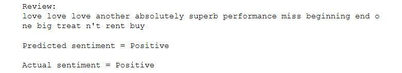
Figure 7.41: A review from the IMDB dataset
Activity 20: Predicting Sentiments from Tweets
Solution:
- Read the tweet dataset using pandas and rename the columns with those given in the following code:
import pandas as pd
data = pd.read_csv('tweet-data.csv', encoding='latin-1', header=None)
data.columns = ['sentiment', 'id', 'date', 'q', 'user', 'text']
- Drop the following columns as we won't be using them. You can analyze and use them if you want when trying to improve the accuracy:
data = data.drop(['id', 'date', 'q', 'user'], axis=1)
- We perform this activity only on a subset (400,000 tweets) of the data to save time. If you want, you can work on the whole dataset:
data = data.sample(400000).reset_index(drop=True)
- Convert the tweets to lowercase to reduce the number of unique words. Keep in mind that "Hello" and "hellow" are not the same to a computer:
data.text = data.text.str.lower()
- Clean the tweets using the clean_str function:
import re
def clean_str(string):
string = re.sub(r"https?://S+", '', string)
string = re.sub(r"@w*s", '', string)
string = re.sub(r'<a href', ' ', string)
string = re.sub(r'&', '', string)
string = re.sub(r'<br />', ' ', string)
string = re.sub(r'[_"-;%()|+&=*%.,!?:#$@[]/]', ' ', string)
string = re.sub('d','', string)
return string
data.text = data.text.apply(lambda x: clean_str(str(x)))
- Remove all the stop words from the tweets, as was done in the Text Preprocessing section:
from nltk.corpus import stopwords
from nltk.tokenize import word_tokenize,sent_tokenize
stop_words = stopwords.words('english')
stop_words = set(stop_words)
remove_stop_words = lambda r: [[word for word in word_tokenize(sente) if word not in stop_words] for sente in sent_tokenize(r)]
data['text'] = data['text'].apply(remove_stop_words)
def combine_text(text):
try:
return ' '.join(text[0])
except:
return np.nan
data.text = data.text.apply(lambda x: combine_text(x))
data = data.dropna(how='any')
- Tokenize the tweets and convert them to numbers using the Keras Tokenizer:
from keras.preprocessing.text import Tokenizer
tokenizer = Tokenizer(num_words=5000)
tokenizer.fit_on_texts(list(data['text']))
sequences = tokenizer.texts_to_sequences(data['text'])
word_index = tokenizer.word_index
- Finally, pad the tweets to have a maximum of 50 words. This will remove any words after the 50-word limit and add 0s if the number of words is less than 50:
from keras.preprocessing.sequence import pad_sequences
tweets = pad_sequences(sequences, maxlen=50)
- Create the embedding matrix from the GloVe embedding file that we downloaded using the load_embedding function:
import numpy as np
def load_embedding(filename, word_index , num_words, embedding_dim):
embeddings_index = {}
file = open(filename, encoding="utf-8")
for line in file:
values = line.split()
word = values[0]
coef = np.asarray(values[1:])
embeddings_index[word] = coef
file.close()
embedding_matrix = np.zeros((num_words, embedding_dim))
for word, pos in word_index.items():
if pos >= num_words:
continue
embedding_vector = embeddings_index.get(word)
if embedding_vector is not None:
embedding_matrix[pos] = embedding_vector
return embedding_matrix
embedding_matrix = load_embedding('../../embedding/glove.twitter.27B.50d.txt', word_index, len(word_index), 50)
- Split the dataset into training and testing sets with an 80:20 spilt. You can experiment with different splits:
from sklearn.model_selection import train_test_split
X_train, X_test, y_train, y_test = train_test_split(tweets, pd.get_dummies(data.sentiment), test_size=0.2, random_state=9)
- Create the LSTM model that will predict the sentiment. You can modify this to create your own neural network:
from keras.models import Sequential
from keras.layers import Dense, Dropout, BatchNormalization, Embedding, Flatten, LSTM
embedding_layer = Embedding(len(word_index),
50,
weights=[embedding_matrix],
input_length=50,
trainable=False)
model = Sequential()
model.add(embedding_layer)
model.add(Dropout(0.5))
model.add(LSTM(100, dropout=0.2))
model.add(Dense(2, activation='softmax'))
model.compile(loss='binary_crossentropy', optimizer='sgd', metrics = ['acc'])
- Train the model. Here, we train it only for 10 epochs. You can increase the number of epochs to try and get a better accuracy:
model.fit(X_train, y_train, validation_data = (X_test, y_test), epochs=10, batch_size=256)
- Check how well the model is performing by predicting the sentiment of a few tweets in the test set:
preds = model.predict(X_test)
review_num = 1
print("Tweet: "+tokenizer.sequences_to_texts([X_test[review_num]])[0])
sentiment = "Positive" if np.argmax(preds[review_num]) else "Negative"
print(" Predicted sentiment = "+ sentiment)
sentiment = "Positive" if np.argmax(y_test.values[review_num]) else "Negative"
print(" Actual sentiment = "+ sentiment)
The output is as follows:
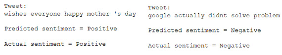
Figure 7.42: Positive (left) and negative (right) tweets and their predictions
Chapter 8: Tips and Tricks of the Trade
Activity 21: Classifying Images using InceptionV3
Solution:
- Create functions to get images and labels. Here PATH variable contains the path to the training dataset.
from PIL import Image
def get_input(file):
return Image.open(PATH+file)
def get_output(file):
class_label = file.split('.')[0]
if class_label == 'dog': label_vector = [1,0]
elif class_label == 'cat': label_vector = [0,1]
return label_vector
- Set SIZE and CHANNELS. SIZE is the dimension of the square image input. CHANNELS is the number of channels in the training data images. There are 3 channels in a RGB image.
SIZE = 200
CHANNELS = 3
- Create a function to preprocess and augment images:
def preprocess_input(image):
# Data preprocessing
image = image.resize((SIZE,SIZE))
image = np.array(image).reshape(SIZE,SIZE,CHANNELS)
# Normalize image
image = image/255.0
return image
- Finally, develop the generator that will generate the batches:
import numpy as np
def custom_image_generator(images, batch_size = 128):
while True:
# Randomly select images for the batch
batch_images = np.random.choice(images, size = batch_size)
batch_input = []
batch_output = []
# Read image, perform preprocessing and get labels
for file in batch_images:
# Function that reads and returns the image
input_image = get_input(file)
# Function that gets the label of the image
label = get_output(file)
# Function that pre-processes and augments the image
image = preprocess_input(input_image)
batch_input.append(image)
batch_output.append(label)
batch_x = np.array(batch_input)
batch_y = np.array(batch_output)
# Return a tuple of (images,labels) to feed the network
yield(batch_x, batch_y)
- Next, we will read the validation data. Create a function to read the images and their labels:
from tqdm import tqdm
def get_data(files):
data_image = []
labels = []
for image in tqdm(files):
label_vector = get_output(image)
img = Image.open(PATH + image)
img = img.resize((SIZE,SIZE))
labels.append(label_vector)
img = np.asarray(img).reshape(SIZE,SIZE,CHANNELS)
img = img/255.0
data_image.append(img)
data_x = np.array(data_image)
data_y = np.array(labels)
return (data_x, data_y)
- Read the validation files:
import os
files = os.listdir(PATH)
random.shuffle(files)
train = files[:7000]
test = files[7000:]
validation_data = get_data(test)
7. Plot a few images from the dataset to see whether you loaded the files correctly:
import matplotlib.pyplot as plt
plt.figure(figsize=(20,10))
columns = 5
for i in range(columns):
plt.subplot(5 / columns + 1, columns, i + 1)
plt.imshow(validation_data[0][i])
A random sample of the images is shown here:
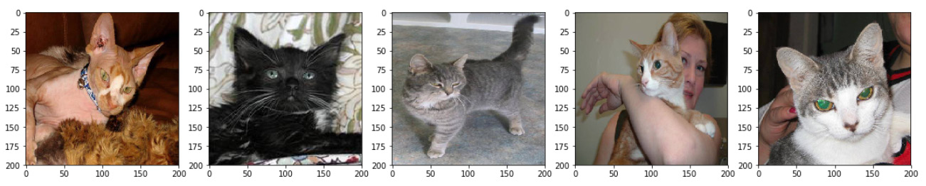
Figure 8.16: Sample images from the loaded dataset
- Load the Inception model and pass the shape of the input images:
from keras.applications.inception_v3 import InceptionV3
base_model = InceptionV3(weights='imagenet', include_top=False, input_shape=(SIZE,SIZE,CHANNELS))
- Add the output dense layer according to our problem:
from keras.layers import GlobalAveragePooling2D, Dense, Dropout
from keras.models import Model
x = base_model.output
x = GlobalAveragePooling2D()(x)
x = Dense(256, activation='relu')(x)
x = Dropout(0.5)(x)
predictions = Dense(2, activation='softmax')(x)
model = Model(inputs=base_model.input, outputs=predictions)
- Next, compile the model to make it ready for training:
model.compile(loss='categorical_crossentropy',
optimizer='adam',
metrics = ['accuracy'])
And then perform the training of the model:
EPOCHS = 50
BATCH_SIZE = 128
model_details = model.fit_generator(custom_image_generator(train, batch_size = BATCH_SIZE),
steps_per_epoch = len(train) // BATCH_SIZE,
epochs = EPOCHS,
validation_data= validation_data,
verbose=1)
- Evaluate the model and get the accuracy:
score = model.evaluate(validation_data[0], validation_data[1])
print("Accuracy: {0:.2f}%".format(score[1]*100))
The accuracy is as follows:
Figure 8.17: Model accuracy
Activity 22: Using Transfer Learning to Predict Images
Solution:
- First, set the random number seed so that the results are reproducible:
from numpy.random import seed
seed(1)
from tensorflow import set_random_seed
set_random_seed(1)
- Set SIZE and CHANNELS
SIZE is the dimension of the square image input. CHANNELS is the number of channels in the training data images. There are 3 channels in a RGB image.
SIZE = 200
CHANNELS = 3
- Create functions to get images and labels. Here PATH variable contains the path to the training dataset.
from PIL import Image
def get_input(file):
return Image.open(PATH+file)
def get_output(file):
class_label = file.split('.')[0]
if class_label == 'dog': label_vector = [1,0]
elif class_label == 'cat': label_vector = [0,1]
return label_vector
- Create a function to preprocess and augment images:
def preprocess_input(image):
# Data preprocessing
image = image.resize((SIZE,SIZE))
image = np.array(image).reshape(SIZE,SIZE,CHANNELS)
# Normalize image
image = image/255.0
return image
- Finally, create the generator that will generate the batches:
import numpy as np
def custom_image_generator(images, batch_size = 128):
while True:
# Randomly select images for the batch
batch_images = np.random.choice(images, size = batch_size)
batch_input = []
batch_output = []
# Read image, perform preprocessing and get labels
for file in batch_images:
# Function that reads and returns the image
input_image = get_input(file)
# Function that gets the label of the image
label = get_output(file)
# Function that pre-processes and augments the image
image = preprocess_input(input_image)
batch_input.append(image)
batch_output.append(label)
batch_x = np.array(batch_input)
batch_y = np.array(batch_output)
# Return a tuple of (images,labels) to feed the network
yield(batch_x, batch_y)
- Next, we will read the development and test data. Create a function to read the images and their labels:
from tqdm import tqdm
def get_data(files):
data_image = []
labels = []
for image in tqdm(files):
label_vector = get_output(image)
img = Image.open(PATH + image)
img = img.resize((SIZE,SIZE))
labels.append(label_vector)
img = np.asarray(img).reshape(SIZE,SIZE,CHANNELS)
img = img/255.0
data_image.append(img)
data_x = np.array(data_image)
data_y = np.array(labels)
return (data_x, data_y)
- Now read the development and test files. The split for the train/dev/test set is 70%/15%/15%.
import random
random.shuffle(files)
train = files[:7000]
development = files[7000:8500]
test = files[8500:]
development_data = get_data(development)
test_data = get_data(test)
- Plot a few images from the dataset to see whether you loaded the files correctly:
import matplotlib.pyplot as plt
plt.figure(figsize=(20,10))
columns = 5
for i in range(columns):
plt.subplot(5 / columns + 1, columns, i + 1)
plt.imshow(validation_data[0][i])
Check the output in the following screenshot:
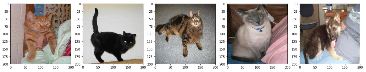
Figure 8.18: Sample images from the loaded dataset
- Load the Inception model and pass the shape of the input images:
from keras.applications.inception_v3 import InceptionV3
base_model = InceptionV3(weights='imagenet', include_top=False, input_shape=(200,200,3))
10. Add the output dense layer according to our problem:
from keras.models import Model
from keras.layers import GlobalAveragePooling2D, Dense, Dropout
x = base_model.output
x = GlobalAveragePooling2D()(x)
x = Dense(256, activation='relu')(x)
keep_prob = 0.5
x = Dropout(rate = 1 - keep_prob)(x)
predictions = Dense(2, activation='softmax')(x)
model = Model(inputs=base_model.input, outputs=predictions)
- This time around, we will freeze the first five layers of the model to help with the training time:
for layer in base_model.layers[:5]:
layer.trainable = False
- Compile the model to make it ready for training:
model.compile(loss='categorical_crossentropy',
optimizer='adam',
metrics = ['accuracy'])
- Create callbacks for Keras:
from keras.callbacks import ModelCheckpoint, ReduceLROnPlateau, EarlyStopping, TensorBoard
callbacks = [
TensorBoard(log_dir='./logs',
update_freq='epoch'),
EarlyStopping(monitor = "val_loss",
patience = 18,
verbose = 1,
min_delta = 0.001,
mode = "min"),
ReduceLROnPlateau(monitor = "val_loss",
factor = 0.2,
patience = 8,
verbose = 1,
mode = "min"),
ModelCheckpoint(monitor = "val_loss",
filepath = "Dogs-vs-Cats-InceptionV3-{epoch:02d}-{val_loss:.2f}.hdf5",
save_best_only=True,
period = 1)]
Note
Here, we are making use of four callbacks: TensorBoard, EarlyStopping, ReduceLROnPlateau, and ModelCheckpoint.
Perform training on the model. Here we train our model for 50 epochs only and with a batch size of 128:
EPOCHS = 50
BATCH_SIZE = 128
model_details = model.fit_generator(custom_image_generator(train, batch_size = BATCH_SIZE),
steps_per_epoch = len(train) // BATCH_SIZE,
epochs = EPOCHS,
callbacks = callbacks,
validation_data= development_data,
verbose=1)
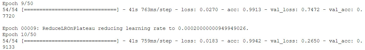
The training logs on TensorBoard are shown here:
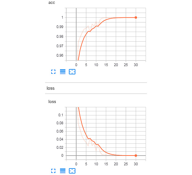
Figure 8.19: Training set logs from TensorBoard
- You can now fine-tune the hyperparameters taking accuracy of the development set as the metric.
The logs of the development set from the TensorBoard tool are shown here:
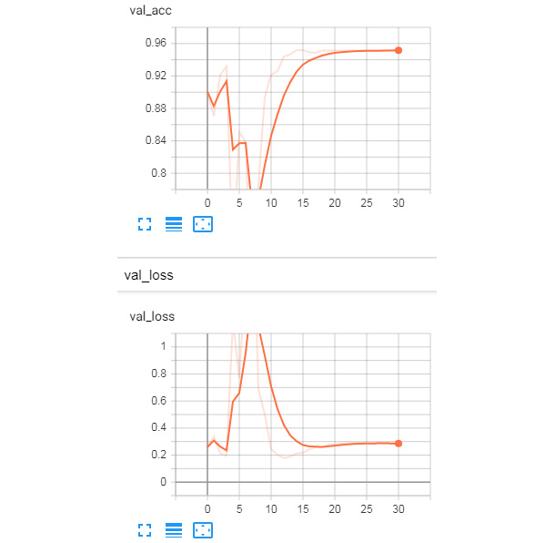
Figure 8.20: Validation set logs from TensorBoard
The learning rate decrease can be observed from the following plot:
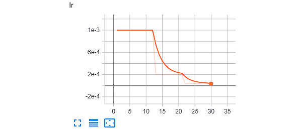
Figure 8.21: Learning rate log from TensorBoard
- Evaluate the model on the test set and get the accuracy:
score = model.evaluate(test_data[0], test_data[1])
print("Accuracy: {0:.2f}%".format(score[1]*100))
To understand fully, refer to the following output screenshot:
Figure 8.22: The final accuracy of the model on the test set
As you can see, the model gets an accuracy of 93.6% on the test set, which is different from the accuracy of the development set (93.3% from the TensorBoard training logs). The early stopping callback stopped training when there wasn't a significant improvement in the loss of the development set; this helped us save some time. The learning rate was reduced after nine epochs, which helped training, as can be seen here: