Chapter 5

Mastering Structured Data

Learning Objectives

By the end of this chapter, you will be able to:

• Work with structured data to create highly accurate models
• Use the XGBoost library to train boosting models
• Use the Keras library to train neural network models
• Fine-tune model parameters to get the best accuracy
• Use cross-validation
• Save and load your trained models

This chapter will cover the basics on how to create highly accurate structured data models.

Introduction

There are two main types of data, structured and unstructured. Structured data refers to data that has a defined format and is usually shaped as a table, such as data stored in an Excel sheet or a relational database. Unstructured data does not have a predefined schema. Anything that cannot be stored in a table falls under this category. Examples include voice files, images, and PDFs.

In this chapter, we will focus on structured data and creating machine learning models using XGBoost and Keras. The XGBoost algorithm is widely used by industry experts and researchers due to the speed at which it delivers high-precision models, and also due to its distributed nature. The distributed nature refers to the ability to process data and train models in parallel; this enables faster training and much shorter turnaround time for data scientists. Keras on the other hand lets us create neural network models. Neural networks work much better than boosting algorithms in some cases, but finding the right network and the right configuration of the network is tough. The following topics will help you get familiar with both libraries, making sure that you can tackle any structured data in your data science journey.

Boosting Algorithms

Boosting is a way to improve the accuracy of any learning algorithm. Boosting works by combining rough, high-level rules into a single prediction that is more accurate than any single rule. Iteratively, a subset of the training dataset is ingested into a "weak" algorithm to generate a weak model. These weak models are then combined to form the final prediction. Two of the most effective boosting algorithms are gradient boosting machine and XGBoost.

Gradient Boosting Machine (GBM)

GBM makes use of classification trees as the weak algorithm. The results are generated by improving estimations from these weak models using a differentiable loss function. The model fits consecutive trees by considering the net loss of the previous trees; therefore, each tree is partially present in the final solution. Hence, boosting trees decreases the speed of the algorithm, and the transparency that they provide gives much better results. The GBM algorithm has a lot of parameters and it is sensitive to noise and extreme values. At the same time, GBM overfits the data, and thus a proper stopping point is required, but it is often the best possible model.

XGBoost (Extreme Gradient Boosting)

XGBoost is the algorithm of choice for researchers across the world when modelling structured data. XGBoost also uses trees as the weak algorithm. So, why is it the first algorithm that comes to mind when data scientists see structured data? XGBoost is portable and distributed, which means that it can be easily used in different architectures and can use multiple cores (single machine) or multiple machines (clusters). As a bonus, the XGBoost library is written in C++, which makes it fast. It is also useful when working with a huge dataset, as it allows you to store data on an external disk and not load all the data on to the memory.

Note

You can read more about XGBoost here: https://arxiv.org/abs/1603.02754

Exercise 44: Using the XGBoost library to Perform Classification

In this exercise, we will perform classification on the wholesale customer dataset (https://github.com/TrainingByPackt/Data-Science-with-Python/tree/master/Chapter05/data) using XGBoost library for Python. The dataset contains purchase data for clients of a wholesale distributor. It includes the annual spending on diverse range of product categories. We will predict the channel based on the annual spend on various products. The channel here describes whether the client is either a horeca (hotel/restaurant/café) or a retail customer.

1. Open the Jupyter Notebook from your virtual environment.
2. Import XGBoost, Pandas, and sklearn for the function that we will use to calculate the accuracy. The accuracy is required to understand how our model is performing.

   import pandas as pd

   import xgboost as xgb from sklearn.metrics import accuracy_score

3. Read the wholesale customer dataset using pandas and check to see if it was loaded successfully using the following command:

   data = pd.read_csv("data/wholesale-data.csv")

4. Check the first five entries of the dataset using the head() command. The output is shown in the following screenshot:

   data.head()

   

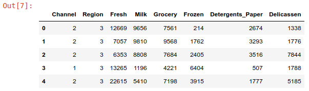
   Figure 5.1: Screenshot showing first five elements of dataset

5. Now the "data" dataframe has all the data. It has the target variable, which is "Channel" in our case, and it has the predictor variables. So, we split the data into features (predictor) and labels (target).

   X = data.copy()X.drop("Channel", inplace = True, axis = 1)Y = data.Channel

6. Create training and test sets as discussed in previous chapters. Here, we use an 80:20 split as the number of data points in the dataset is less. You can experiment with different splits.

   X_train, X_test = X[:int(X.shape[0]*0.8)].values, X[int(X.shape[0]*0.8):].values Y_train, Y_test = Y[:int(Y.shape[0]*0.8)].values, Y[int(Y.shape[0]*0.8):].values

7. Convert the pandas dataframe into a DMatrix, an internal data structure that is used by XGBoost to store training and testing datasets.

   train = xgb.DMatrix(X_train, label=Y_train)test = xgb.DMatrix(X_test, label=Y_test)

8. Specify the training parameters and train the model.

   Note

   We will go over these parameters in depth in the next section.

   param = {'max_depth':6, 'eta':0.1, 'silent':1, 'objective':'multi:softmax', 'num_class': 3}num_round = 5 model = xgb.train(param, train, num_round)

   Note

   By default, XGBoost uses all threads available to it for multiprocessing. To limit this, you can use the nthread parameter. Refer the next section for more information.

9. Predict the "Channel" values of the test set using the model that we just created.

   preds = model.predict(test)

10. Get the accuracy of the model that we have trained for the test dataset.

    acc = accuracy_score(Y_test, preds)print("Accuracy: %.2f%%" % (acc * 100.0))

    The output screenshot is as follows:

Figure 5.2: Final accuracy

Congratulations! You just made your first XGBoost model with approximately 90% accuracy without much fine-tuning!

XGBoost Library

The library we used to perform the above classification is named XGBoost. The library enables a lot of customization using the many parameters it has. In the following sections, we will dive in and understand the different parameters and functions of the XGBoost library.

Note

For more information about XGBoost, refer the website: https://xgboost.readthedocs.io

Training

Parameters that affect the training of any XGBoost model are listed below.

• booster: Even though we mentioned in the introduction that the base learner of XGBoost is a regression tree, using this library, we can use linear regression as the weak learner as well. Another weak learner, DART booster, is a new method to tree boosting, which drops trees at random to prevent overfitting. To use tree boosting, pass "gbtree" (default); for linear regression, pass "gblinear"; and for tree boosting with dropout, pass "dart".

  Note

  You may learn more about DART from this paper: http://www.jmlr.org/proceedings/papers/v38/korlakaivinayak15.pdf

• silent: 0 prints the training logs, whereas 1 is the silent mode.
• nthread: This signifies the number of parallel threads to be used. It defaults to the maximum number of threads available in the system.

  Note

  The parameter silent has been deprecated and has been replaced with verbosity, which takes any of the following values: 0 (silent), 1 (warning), 2 (info), 3 (debug).

• seed: This is the seed value for the random number generator. Set a constant value here to get reproducible results. The default value is 0.
• objective: This is a function that the model tries to minimize. The next few points cover the objective functions.

  reg:linear: Linear regression should be used with continuous target variables (regression problem). (Default)

  binary:logistic: logistic regression to be used in case of binary classification. It outputs probability and not classes.

  binary:hinge: This is binary classification that outputs predictions of 0 or 1, rather than the probabilities. Use this when you are not concerned about the probabilities.

  multi:softmax: If you want to do a multiclass classification, use this to perform the classification using the softmax objective. It is mandatory to set the num_class parameter to the number of classes for this.

  multi:softprob: This works the same as softmax, but the outputs predict the probability of each data point instead of predicting a class.

• eval_metric: The performance of a model needs to be observed on the validation set (as discussed in Chapter 1, Introduction to Data Science and Data Preprocessing). This parameter takes the evaluation metric for the validation data. The default metric is chosen according to the objective function (rmse for regression and logloss for classification). You can use multiple evaluation metrics.

  rmse: Root mean square error (RMSE) penalizes large errors more. So, it is appropriate when being off by 1 is more than three times as bad as being off by 3.

  mae: Mean absolute error (MAE) can be used in cases where being off by 1 is similar to being off by 3.

  The following graph shows the increase in the error with the increase in difference between the actual and predicted values. Here, it would be the following:

Figure 5.3: Difference between actual and predicted value

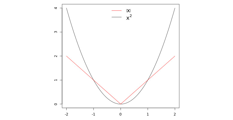
Figure 5.4: Variation of penalty with variation in error; |X| is mae and X2 is rmse

logloss: The negative log-likelihood, logloss is a classification loss function. Minimising the logloss of a model is equivalent to maximising the model's accuracy. It is defined mathematically as:

Figure 5.5: Logloss equation diagram

Here, N is the number of data points, M is the number of classes and is either 1 or 0 depending on whether the prediction was correct or not, is the probability of predicting label j for data point i.

AUC: Area under the curve is used widely for binary classification. You should always use this if your dataset has a class imbalance problem. A class imbalance problem occurs when your data is not split up into classes of similar sizes; for example, if class A makes up 90% of the data and class B makes up 10% of the data. We will talk more about the class imbalance problem in the Handling Imbalanced Datasets section.

aucpr: Area under the precision-recall (PR) curve is the same as the AUC curve, but should be preferred in case of a highly imbalanced dataset. We shall discuss this too in the Handling Imbalanced Datasets section.

Note

AUC or AUCPR should be used as a rule of thumb whenever you are working with a binary dataset.

Tree Booster

Parameters that are specific to tree-based models are listed below:

• eta: This is the learning rate. Modify this value to prevent overfitting as discussed in Chapter 1, Introduction to Data Science and Data Preprocessing. The learning rate decides by how much the weights will get updated in each step. The gradient of weights gets multiplied by this and then added to the weight. This defaults to 0.3 and has a maximum value of 1 and a minimum value of 0.
• gamma: This is the minimum loss reduction to make a partition. The larger gamma is, the more conservative the algorithm will be. Being more conservative prevents overfitting. The value depends on the dataset and other parameters used. It ranges from 0 to infinity and the default value is 0. A lower value leads to shallow trees and larger values give rise to deeper trees.

  Note

  Gamma values above 1 usually do not give good results.

• max_depth: This is the maximum depth of any tree as discussed in Chapter 3, Introduction to ML via Sklearn. Increasing the max depth will make the model more likely to overfit. 0 means no limit. It defaults to 6.
• subsample: Setting this to 0.5 will cause the algorithm to randomly sample half of the training data before growing the trees. This prevents overfitting. Subsampling occurs once every boosting iteration and defaults to 1, which makes the model take the complete dataset and not a sample.
• lambda: This is the L2 regularization term. L2 regularization adds a squared magnitude of the coefficient as the penalty term to the loss function. Increasing this value prevents overfitting. Its default value is 1.
• alpha: This is the L1 regularization term. L1 regularization adds an absolute magnitude of the coefficient as the penalty term to the loss function. Increasing this value prevents overfitting. Its default value is 0.
• scale_pos_weight: This is useful when the classes are highly imbalanced. We will learn more about imbalanced data in the following sections. A typical value to consider introducing: the sum of negative instances / the sum of positive instances. Its default value is 1.
• predictor: There are two predictors. cpu_predictor uses CPU for prediction. It is the default. gpu_predictor uses GPU for prediction.

  Note

  Get a list of all the parameters here: https://xgboost.readthedocs.io/en/latest/parameter.html

Controlling Model Overfitting

If you observe high accuracy on the training dataset but a low accuracy on the test dataset, your model has overfit to the training data, as seen in Chapter 1, Introduction to Data Science and Data Preprocessing. There are two main ways to limit overfitting in XGBoost:

• Control model complexity: Modify max_depth, min_child_weight, and gamma while monitoring the training and test metrics to get the best model without overfitting to the training dataset. You will learn more about this in the following sections.
• Add randomness to the model to make training it robust to noise: Use the subsample parameter to get a subsample of the training data. Setting the parameter subsample to 0.5 will make the library randomly sample half of the training dataset before creating the weak models. colsample_bytree does the same thing as subsampling but with columns instead of rows.

To understand better, see the training and accuracy graphs in the following figure:

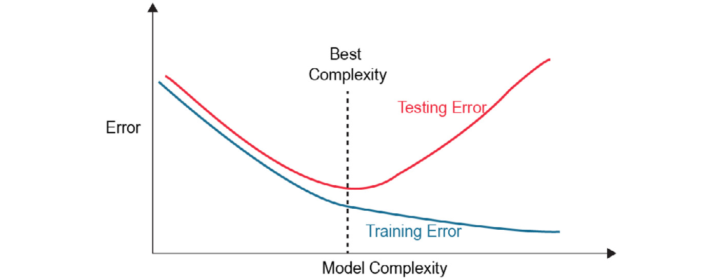
Figure 5.6: Training and accuracy graphs

To understand the conceptualization of a dataset with overfit and proper-fit models, refer to the following figure:

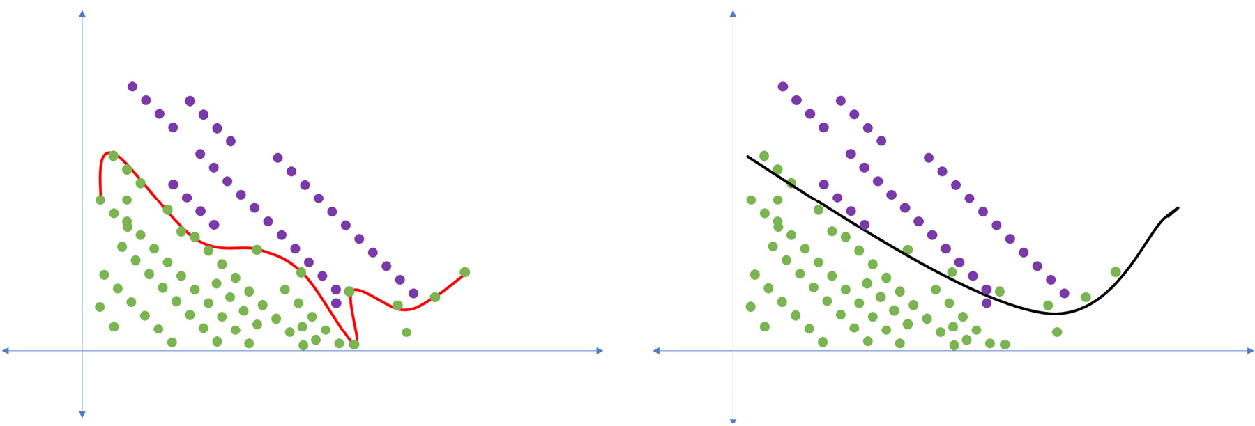
Figure 5.7: Illustration of a dataset with overfit and proper-fit models

Note

The black line represents the model that has a proper fit, whereas the model represented by the red line has overfit the dataset.

Handling Imbalanced Datasets

Imbalanced datasets cause a lot of problems to data scientists. One example of an imbalanced dataset is credit card fraud data. Here, about 95% of transactions will be legitimate and only 5% will be fraudulent. In this case, a model that predicts every transaction to be a correct transaction will get 95% accuracy, but, it is a very bad model. To see the distribution of your classes, you can use the following function:

data['target_variable'].value_counts()

The output would be as follows:

Figure 5.8: Class distribution

To handle imbalanced datasets, you can use the following methods:

• Undersample the class that has a higher number of records: In the case of credit card fraud, you can randomly sample legitimate transactions to get records equal to the fraudulent records. This will result in equal distribution of the two classes, fraudulent and legitimate.
• Oversample the class that has lesser records: In the case of credit card fraud, you can introduce more samples of the fraudulent transactions by adding either new data points or by copying the existing data points. This will result in equal distribution of the two classes, fraudulent and legitimate.
• Balance the positive and negative weights with scale_pos_weight: You can use this parameter to allot a higher weight to the class with a smaller number of data points and thus artificially balance the classes. The value of the parameter can be:

Figure 5.9: Value parameter equation

You can check the distribution of the classes using the following code:

positive = sum(Y == 1)

negative = sum(Y == 0)

scale_pos_weight = negative/positive

• Use AUC or AUCPR for evaluation: As mentioned earlier, the AUC and AUCPR metrics are sensitive to imbalanced dataset, unlike accuracy, which gives you a high value for a bad model that predicts the majority class most of the time. AUC can be plotted only for binary classification problems. It is a representation of the True Positive Rate vs. the False Positive Rate at different thresholds (0, 0.01, 0.02… 1) of the predicted value. It is shown in the following figure:

Figure 5.10: TPR and FPR equations

The metric is the area under the curve that we get after plotting TPR and FPR. When dealing with highly skewed datasets, AUCPR gives a better picture and is thus preferred. AUCPR is the representation of precision and recall at different thresholds

Figure 5.11: Precision and recall equations

As a rule of thumb, you should use AUC or AUCPR as the evaluation metric when dealing with imbalanced classes as it gives a clearer picture of the model.

Note

Machine learning algorithms cannot easily process strings or categorical variables represented as strings, so we have to convert them into numbers.

Activity 14: Training and Predicting the Income of a Person

In this activity, we will attempt to predict whether or not the income of an individual exceeds $50,000. The adult income dataset (https://github.com/TrainingByPackt/Data-Science-with-Python/tree/master/Chapter05/data) has its data sourced from the 1994 census dataset (https://archive.ics.uci.edu/ml/datasets/adult) and contains information such as income, education qualification of a person, and their occupation. Let's look at the following scenario: You work at a car company and you need to create a system by which the sales representatives of your firm can figure out what kind of car to sell to which person.

To do this, you create a machine learning model that predicts the income of a prospective buyer and thus provides the salesperson with the right information to sell the right car.

1. Load the income dataset (adult-data.csv) using pandas.
2. The data should look like this:
   

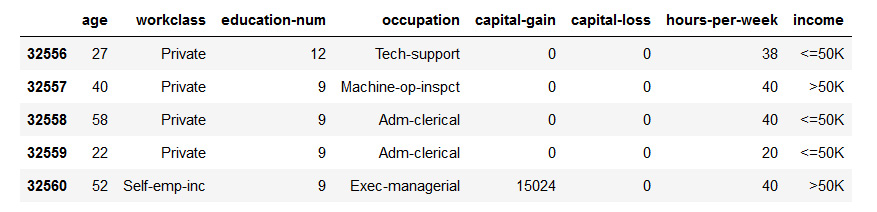
   Figure 5.12: Screenshot showing five elements of census dataset

   Use the following code to specify column names:

   data = pd.read_csv("../data/adult-data.csv", names=['age', 'workclass','education-num', 'occupation', 'capital-gain', 'capital-loss', 'hoursper-week', 'income'])

3. Convert all the categorical variables from strings to integers using sklearn.
4. Perform prediction using the XGBoost library and perform parameter tuning to improve the accuracy to be more than 80%.

We have successfully predicted the income using the dataset with around 83% accuracy.

Note

The solution for this activity can be found on page 360.

External Memory Usage

When you have an exceptionally large dataset that you can't load on to your RAM, the external memory feature of the XGBoost library will come to your rescue. This feature will train XGBoost models for you without loading the entire dataset on the RAM.

Using this feature requires minimal effort; you just need to add a cache prefix at the end of the filename.

train = xgb.DMatrix('data/wholesale-data.dat.train#train.cache')

This feature supports only libsvm file. So, we will now convert a dataset loaded in pandas into a libsvm file to be used with the external memory feature.

Note

You might have to do this in batches depending on how big your dataset is.

from sklearn.datasets import dump_svmlight_file

dump_svmlight_file(X_train, Y_train, 'data/wholesale-data.dat.train', zero_based=True, multilabel=False)

Here, X_train and Y_train are the predictor and target variables respectively. The libsvm file will get saved into the data folder.

Cross-validation

Cross-validation is a technique that helps data scientists evaluate their models on unseen data. It is helpful when your dataset isn't large enough to create three splits (training, testing, and validation). Cross-validation helps the model avoid overfitting by presenting it with different partitions of the same data. It works by feeding different training and validation sets of the dataset for every pass of cross-validation. 10-fold cross-validation is the most used, where the dataset is divided into 10 completely different subsets and is trained on each one of them, and finally, the metrics are averaged out to obtain the accurate prediction performance of the model. In every round of cross-validation, we do the following:

1. Shuffle the dataset and split it into k different groups (k=10 for 10-fold cross-validation).
2. Train the model on k-1 groups and test it on 1 group.
3. Evaluate the model and store the results.
4. Repeat steps 2 and 3 with different groups until all k combinations are trained.
5. The final metric is the mean of the metrics generated in the different rounds.

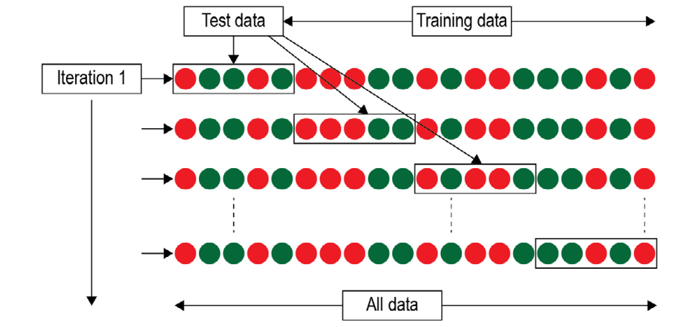
Figure 5.13: Illustration of a cross-validation dataset

The XGBoost library has an inbuilt function to perform cross-validation. This section will help you get you familiar using it.

Exercise 45: Using Cross-validation to Find the Best Hyperparameters

In this exercise, we will find the best hyperparameters for the adult dataset from the previous activity using the XGBoost library for Python. To do this, we will make use of the cross-validation feature of the library.

1. Load the census dataset from Activity 14 and perform all the preprocessing steps.

   import pandas as pd

   import numpy as np

   data = pd.read_csv("../data/adult-data.csv", names=['age', 'workclass', 'fnlwgt', 'education-num', 'occupation', 'capital-gain', 'capital-loss', 'hours-per-week', 'income'])

   Use Label Encoder from sklearn to encode strings. First, import Label Encoder, then encode all the string categorical columns one by one.

   from sklearn.preprocessing import LabelEncoder

   data['workclass'] = LabelEncoder().fit_transform(data['workclass'])

   data['occupation'] = LabelEncoder().fit_transform(data['occupation'])

   data['income'] = LabelEncoder().fit_transform(data['income'])

2. Make train and test sets from the data and convert the data into Dmatrix.

   import xgboost as xgb

   X = data.copy()

   X.drop("income", inplace = True, axis = 1)

   Y = data.income

   X_train, X_test = X[:int(X.shape[0]*0.8)].values, X[int(X.shape[0]*0.8):].values

   Y_train, Y_test = Y[:int(Y.shape[0]*0.8)].values, Y[int(Y.shape[0]*0.8):].values

   train = xgb.DMatrix(X_train, label=Y_train)

   test = xgb.DMatrix(X_test, label=Y_test)

3. Instead of using the train function, use the following code to perform 10-fold cross-validation and store the result in the model_metrics dataframe. The for loop iterates over different tree depth values to find the best one for our dataset.

   test_error = {}

   for i in range(20):

       param = {'max_depth':i, 'eta':0.1, 'silent':1, 'objective':'binary:hinge'}

       num_round = 50

       model_metrics = xgb.cv(param, train, num_round, nfold = 10)

       test_error[i] = model_metrics.iloc[-1]['test-error-mean']

4. Visualize the results using Matplotlib.

   import matplotlib.pyplot as plt

   plt.scatter(test_error.keys(),test_error.values())

   plt.xlabel('Max Depth')

   plt.ylabel('Test Error')

   plt.show()

   

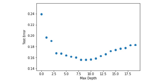
   Figure 5.14: Graph of max depth with test error

   From the graph, we understand that the max depth of 9 works best for our dataset as it has the lowest test error.

5. Find the best learning rate. Running this piece of code will take a while as it iterates over a lot of learning rates for 500 rounds each.

   for i in range(1,100,5):

       param = {'max_depth':9, 'eta':0.001*i, 'silent':1, 'objective':'binary:hinge'}

       num_round = 500

       model_metrics = xgb.cv(param, train, num_round, nfold = 10)

       test_error[i] = model_metrics.iloc[-1]['test-error-mean']

6. Visualize the results.

   lr = [0.001*(i) for i in test_error.keys()]

   plt.scatter(temp,test_error.values())

   plt.xlabel('Learning Rate')

   plt.ylabel('Error')

   plt.show()

   

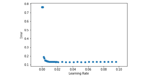
   Figure 5.15: Graph of learning rate with test error

   From the graph, we can see that a learning rate of about 0.01 works best for our model as it has the lowest error.

7. Let us visualize the training and testing errors for each round for the learning rate 0.01.

   param = {'max_depth':9, 'eta':0.01, 'silent':1, 'objective':'binary:hinge'}

   num_round = 500

   model_metrics = xgb.cv(param, train, num_round, nfold = 10)

   plt.scatter(range(500),model_metrics['test-error-mean'], s = 0.7, label = 'Test Error')

   plt.scatter(range(500),model_metrics['train-error-mean'], s = 0.7, label = 'Train Error')

   plt.legend()

   plt.show()

   

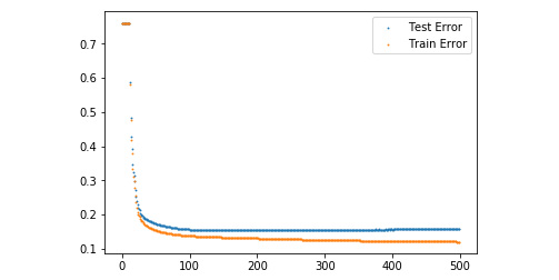
   Figure 5.16: Graph of training and testing errors with respect to number of rounds

   Note

   From this graph, we can see that we get the least error around round 490. This means that our model performs the best when the number of rounds is around 490. Creating this curve helps us create more accurate models.

   To check the least error, use the following code:

   list(model_metrics['test-error-mean']).index(min(model_metrics['test-error-mean']))

8. To understand, check out the output.

Figure 5.17: Least error

Note

The final model parameters that work best for this dataset:

Max depth = 9

Learning rate = 0.01

Number of rounds = 496

Saving and Loading a Model

The last piece in mastering structured data is the ability to save and load the models that you have trained and fine-tuned. Training a new model every time we need a prediction will waste a lot of time, so being able to save a trained model is imperative for data scientists. The saved model allows us to replicate the results and to create apps and services that make use of the machine learning model. The steps are as follows:

1. To save an XGBoost model, you need to call the save_model function.

   model.save_model('wholesale-model.model')

2. To load a previously saved model, you have to call load_model on an initialized XGBoost variable.

   loaded_model = xgb.Booster({'nthread': 2})

   loaded_model.load_model('wholesale-model.model')

   Note

   If you give XGBoost access to all the threads it can get, your computer might become slow while training or predicting.

You are now ready to get started on modeling your structured dataset using the XGBoost library!

Exercise 46: Creating a Python Pcript that Predicts Based on Real-time Input

In this exercise, we will first create a model and save it. We will then create a Python script that will make use of this saved model to perform predictions on the data input by the user.

1. Load the income dataset from Activity 14 as a pandas dataframe.

   import pandas as pd

   import numpy as np

   data = pd.read_csv("../data/adult-data.csv", names=['age', 'workclass', 'education-num', 'occupation', 'capital-gain', 'capital-loss', 'hours-per-week', 'income'])

2. Strip away all trailing spaces.

   data[['workclass', 'occupation', 'income']] = data[['workclass', 'occupation', 'income']].apply(lambda x: x.str.strip())

3. Convert all the categorical variables from strings to integers using scikit.

   from sklearn.preprocessing import LabelEncoder

   from collections import defaultdict

   label_dict = defaultdict(LabelEncoder)

   data[['workclass', 'occupation', 'income']] = data[['workclass', 'occupation', 'income']].apply(lambda x: label_dict[x.name].fit_transform(x))

4. Save the label encoder in a pickle file for future use. A pickle file stores Python objects so that we can access them later when we need them.

   import pickle

   with open( 'income_labels.pkl', 'wb') as f:

           pickle.dump(label_dict, f, pickle.HIGHEST_PROTOCOL)

5. Split the dataset into training and testing and create the model.
6. Save the model to a file.

   model.save_model('income-model.model')

7. In a Python script, load the model and the label encoder.

   import xgboost as xgb

   loaded_model = xgb.Booster({'nthread': 8})

   loaded_model.load_model('income-model.model')

   def load_obj(file):

         with open(file + '.pkl', 'rb') as f:

               return pickle.load(f)

   label_dict = load_obj('income_labels')

8. Read the input from the user.

   age = input("Please enter age: ")

   workclass = input("Please enter workclass: ")

   education_num = input("Please enter education_num: ")

   occupation = input("Please enter occupation: ")

   capital_gain = input("Please enter capital_gain: ")

   capital_loss = input("Please enter capital_loss: ")

   hours_per_week = input("Please enter hours_per_week: ")

9. Create a dataframe to store this data.

   data_list = [age, workclass, education_num, occupation, capital_gain, capital_loss, hours_per_week]

   data = pd.DataFrame([data_list])

   data.columns = ['age', 'workclass', 'education-num', 'occupation', 'capital-gain', 'capital-loss', 'hours-per-week']

10. Preprocess the data.

    data[['workclass', 'occupation']] = data[['workclass', 'occupation']].apply(lambda x: label_dict[x.name].transform(x))

11. Convert into Dmatrix and perform prediction using the model.

    data = data.astype(int)

    data_xgb = xgb.DMatrix(data)

    pred = loaded_model.predict(data_xgb)

12. Perform inverse transformation to get the results.

    income = label_dict['income'].inverse_transform([int(pred[0])])

    The output is as follows:

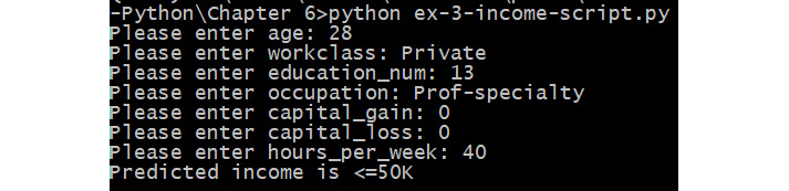
Figure 5.18: Inverse transformation output

Note

Make sure that the values of workclass and occupation that you enter as input are present in the training data, otherwise the script will throw an error. This error occurs when the LabelEncoder encounters a new value it has not seen before.

Congratulations! You built a script that predicts the outcome using user input data. You will now be able to deploy your models anywhere you want to.

Activity 15: Predicting the Loss of Customers

In this activity, we will attempt to predict whether a customer will move to another telecom provider. The data is sourced from IBM sample datasets. Let's look at the following scenario: You work at a telecom company, and recently, a lot of your users have started moving to other providers. Now, to be able to give defecting customers a price cut, you need to predict which customer is the most likely to defect before they do so. To do this, you need to create a machine learning model that predicts which customer will defect.

1. Load the telecom churn (telco-churn.csv) dataset (https://github.com/TrainingByPackt/Data-Science-with-Python/tree/master/Chapter05/data) using pandas. This dataset contains information about the customers of a telecom provider. The original source of the dataset is at: https://www.ibm.com/communities/analytics/watson-analytics-blog/predictive-insights-in-the-telco-customer-churn-data-set/. It contains multiple fields such as charges, tenure, and streaming information, along with a variable that tells us if the customer churned or not. The first few rows should look like this:
   

   Figure 5.19: Screenshot showing first five elements of telecom churn dataset

2. Remove unnecessary variables.
3. Convert all the categorical variables from strings to integers using scikit. You can use the following code: data.TotalCharges = pd.to_numeric(data.TotalCharges, errors='coerce')
4. Fix the data type mismatch when loading with pandas.
5. Perform prediction using the XGBoost library and perform parameter tuning using cross-validation to improve accuracy to be more than 80%.
6. Save your model for future use.

   Note

   The solution for this activity can be found on page 361.

Neural Networks

A neural network is one of the most popular machine learning algorithms available to data scientists. It has consistently outperformed traditional machine learning algorithms in problems where images or digital media are required to find the solution. Given enough data, it outperforms traditional machine learning algorithms in structured data problems. Neural networks that have more than 2 layers are referred to as deep neural networks and the process of using these "deep" networks to solve problems is referred to as deep learning. Two handle unstructured data there are two main types of neural networks: a convolutional neural network (CNN) can be used to process images and a recurrent neural network (RNN) can be used to process time series and natural language data. We will talk more about CNNs and RNNs in Chapter 6, Decoding Images and Chapter 7, Processing Human Language. Let us now see how a vanilla neural network really works. In this section, we will go over the different parts of a neural network in brief. We will explain each topic in detail in the following chapters.

What Is a Neural Network?

The basic unit of a neural network is a neuron. The inspiration for neural networks was taken from the biological brain, which is where the name neuron was inspired from. All connections in the neural network, like the synapses in the brain, can transmit information from one neuron to another. In a neural network, a weighted combination of the input signal is aggregated, and the output signal is then transmitted forward after passing it through a function. This function is a nonlinear activation function and is the neuron's activation threshold. Multiple layers of these interconnected neurons form a neural network. Only the non-output layers of a neural network include bias units. The weights associated with every neuron along with these biases determine the output of the entire network; hence, these are the parameters we modify to fit the data during training.

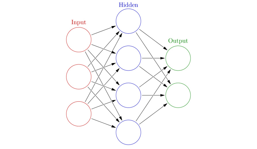
Figure 5.20: Representation of single layer neural network

The first layer of the neural network has nodes equal to the number of independent variables in the dataset. This layer is thus called the input layer, which is followed by multiple hidden layers, at the end of which is the output layer. Each neuron of the input layer takes in one independent variable of the dataset. The output layer outputs the final prediction. These outputs can be continuous (such as 0.2, 0.6, 0.8) if it is a regression problem or categorical (such as 2, 4, 5) if it is a classification problem. The training of a neural network modifies the weights and biases of the network to minimize the error, which is the difference between the expected and the output values. Weights are multiplied with the input to the neuron and then the bias value is added to the combination of these weights to get the output.

Figure 5.21: Neuron output

Here, y is the output of the neuron and x the input, w and b are the weights and bias respectively, and f is the activation function, which we will learn more about later.

Optimization Algorithms

To minimize the error of the model, we train the neural network to minimize a predefined loss function using an optimization algorithm. There are many choices for this optimization algorithm, and you can choose one depending on your data and model. For most of this book, we will work with stochastic gradient descent (SGD), which works well in most cases, but we will explain other optimizers as and when they are required. SGD works by iteratively finding out the gradient, which is the change in the weights with respect to the error. In mathematical terms, it is the partial derivative with respect to the inputs. It finds the gradient that would help it minimize a given function, which in our case is called the loss function. As we get closer to the solution, this gradient reduces in magnitude, thus preventing us from overshooting the optimal solution.

The most intuitive way to understand SGD is the act of descending the bottom of a valley. Initially, we take steep descents, and then when we are close to the bottom, the slope reduces.

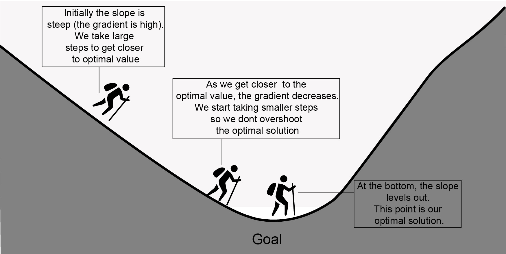
Figure 5.22: Intuition of gradient descent (k represents magnitude of gradient)

Hyperparameters

A big parameter that determines the time required to train a model is called the learning rate, which essentially is the size of the step that we take to perform the descent. Too small a step, and it will take the model a long time to get to the optimal solution; too big, and it will overshoot the optimal solution. To circumvent this, we start with a large learning rate and reduce the learning rate after a few steps. This helps us reach the minimum point faster, and due to the reduction in step size, prevents the model from overshooting the solution.

Next is the initialization of the weights. We need to perform initialization of the weights of a neural network to have a starting point from where we can then modify the weights to minimize the error. Initialization plays a major role in preventing the vanishing and exploding gradient problems.

Vanishing gradient problem refers to the reducing gradients with every layer as the product of any number smaller than 1 is even smaller, so over multiple layers, this value becomes 0.

Exploding gradient problem occurs when large error gradients add up and result in a very large update to the model. If the model loss goes to NaN, this could be a problem.

Using the Xavier initialization, we can prevent these problems as it factors the size of the network while initializing the weights. The Xavier initialization initializes the weights, drawing them from a truncated normal distribution centered on 0 with standard deviation

Figure 5.23: Standard deviation that the Xavier initialization uses.

Where xi is the number of input neurons and yi is the number of output neurons for that layer

This ensures that the variance of both the inputs and the outputs remains the same even if the number of layers in the network is very large.

Loss Function

Another hyperparameter to consider is the loss function. Different loss functions are used depending on the type of the problem, classification or regression. For classification, we choose loss functions such as cross entropy and hinge. For regression, we use loss functions such as mean squared error, mean absolute error (MAE), and Huber. Different functions work well with different datasets. We will go over them as we use them.

Activation Function

While creating the neural network layers, you will have to define an activation function, which depends on whether the layer is a hidden layer or an output layer. In the case of a hidden layer, we will use the ReLU or the tanh activation functions. Activation functions help the neural network model non-linear functions. Almost no real-life situation can be solved using a linear model. Now, apart from this, different activation functions have different features. Sigmoid output has values between 0 and 1, whereas tanh centers the output around 0, which enables better learning. ReLU on the other hand prevents the vanishing gradient problem and is computationally efficient. This is the representation of a ReLU graph.

Figure 5.24: Representation of ReLU activation function

Softmax outputs probabilities and is used when multiclass classification is being performed, whereas sigmoid outputs a value between 0 and 1 and is used only for binary classification. Linear activation is mostly used for models that solve the regression problem. A representation of the sigmoid activation function is shown in the following figure:

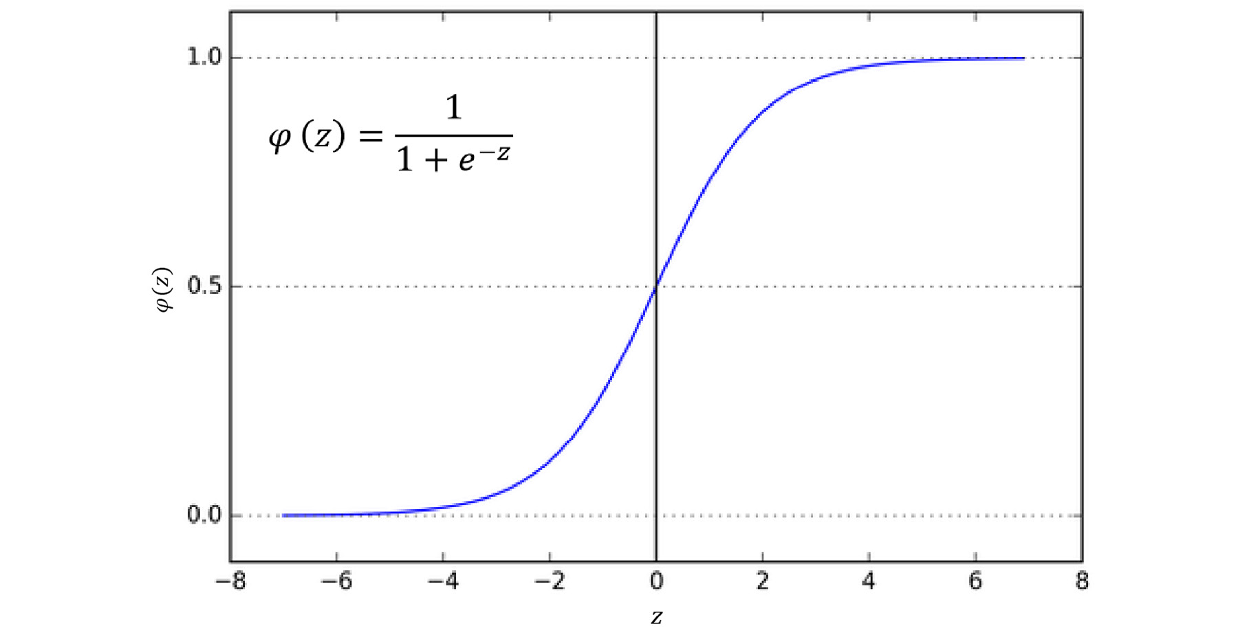
Figure 5.25: Representation of sigmoid activation function

The previous section had a lot of new information; if you are confused, do not worry. We will apply all these concepts practically in the rest of the chapters, which will reinforce all these topics.

Keras

Keras is an open-source, high-level neural network API written in Python. It is capable of running on top of TensorFlow, Microsoft Cognitive Toolkit (CNTK), or Theano. Keras was developed to enable fast experimentation and thus help in rapid application development. Using Keras, one can get from idea to result with the least possible delay. Keras supports almost all the latest data science models relating to neural networks due to the huge community support. It contains multiple implementations of commonly used building blocks such as layers, batch normalization, dropout, objective functions, activation functions, and optimizers. Also, Keras allows users to create models for smartphones (Android and iOS), the web, or for the Java Virtual Machine (JVM). With Keras, you can train your models on your GPU without any change in code.

Given all these features of Keras, it is imperative for data scientists to learn how to use all the different aspects of the library. Mastering the use of Keras will help you tremendously in your journey as a data scientist. To demonstrate the power of Keras, we will now install it and create a single layer neural network model.

Note

You can read more about Keras here: https://keras.io/

Exercise 47: Installing the Keras library for Python and Using it to Perform Classification

In this exercise, we will perform classification on the wholesale customer dataset (which we used in Exercise 44), using the Keras library for Python.

1. Run the following command in your virtual environment to install Keras.

   pip3 install keras

2. Open Jupyter Notebook from your virtual environment.
3. Import Keras and other required libraries.

   import pandas as pd

   from keras.models import Sequential

   from keras.layers import Dense

   import numpy as np

   from sklearn.metrics import accuracy_score

4. Read the wholesale customer dataset using pandas and check to see if it was loaded successfully using the following command:

   data = pd.read_csv("data/wholesale-data.csv")

   data.head()

   The output should look like this:

   

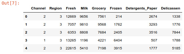
   Figure 5.26: Screenshot showing first five elements of dataset

5. Split the data into features and labels.

   X = data.copy()X.drop("Channel", inplace = True, axis = 1)Y = data.Channel

6. Create training and test sets.

   X_train, X_test = X[:int(X.shape[0]*0.8)].values, X[int(X.shape[0]*0.8):].values Y_train, Y_test = Y[:int(Y.shape[0]*0.8)].values, Y[int(Y.shape[0]*0.8):].values

7. Create the neural network model.

   model = Sequential()

   model.add(Dense(units=8, activation='relu', input_dim=7))

   model.add(Dense(units=16, activation='relu'))

   model.add(Dense(units=1, activation='sigmoid'))

   Here, we create a four-layer network, with one input layer, two hidden layers, and one output layer. The hidden layers have ReLU activation and the output layer has softmax activation.

8. Compile and train the model. We use the binary cross-entropy loss function, which is the same as the logloss we discussed before; we have chosen the optimizer to be stochastic gradient descent. We run the training for five epochs with a batch size of eight.

   model.compile(loss='binary_crossentropy',

                 optimizer='sgd',

                 metrics=['accuracy'])

   model.fit(X_train, Y_train, epochs=5, batch_size=8)

   Note

   You will see the model training log. Epoch refers to the training iteration, and 352 refers to the size of the dataset divided by the batch size. After the progress bar, you can see the time taken for one iteration. Next to that, you see the average time taken to train each batch. Next comes the loss of the model, which over here is the binary cross-entropy loss, followed by the accuracy after the iteration. A few of these terms are new, but we will understand each of them in the following sections.

   

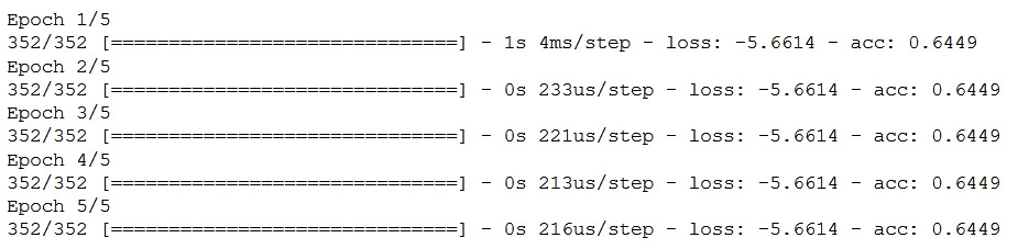
   Figure 5.27: Screenshot of model training logs

9. Predict the values of the test set.

   preds = model.predict(X_test, batch_size=128)

10. Obtain the accuracy of the model.

    accuracy = accuracy_score(Y_test, preds.astype(int))

    print("Accuracy: %.2f%%" % (accuracy * 100.0))

    The output is as follows:

Figure 5.28: Output accuracy

Congratulations! You just made your first neural network model with around 81% accuracy, without any fine-tuning! You will notice that this accuracy is quite low when compared with XGBoost. In the following sections, you will figure out how to improve this accuracy. A major reason for the low accuracy is the size of the data. For a neural network model to really shine, it must have a large dataset to train on; otherwise, it overfits the data.

Keras Library

Keras enables modularity. All initializers, cost functions, optimizers, layers, regularizers, and activation functions are standalone modules that can be used for any type of data and network architecture. You will find almost all the latest functions already implemented in Keras. This allows reusability of code and enables fast experimentation. You as a data scientist are not limited by the inbuilt modules; it is extremely easy to create your own custom modules and use them with other inbuilt modules. This enables research and helps with different use cases. For example, you might have to write a custom loss function to maximize the volume of cars sold, giving more weight to cars that have bigger margins, leading to higher profits.

All the different kinds of layers that you would need to create a neural network are defined in Keras. We will investigate them as we use them. There are two main ways to create neural models in Keras, the sequential model and the functional API.

Sequential: The sequential model is a linear stack of layers. This is the easiest way to create neural network models with Keras. A snippet of this model is given below:

model = Sequential()model.add(Dense(128, input_dim=784))model.add(Activation('relu'))

model.add(Dense(10))model.add(Activation('softmax'))

Functional API: Functional API is the way to go for complex models. Due to the linear nature of the sequential model, creating a complex model is not possible. The functional API lets you create multiple parts of the model and then merge them together. The same model in the functional API is given below:

inputs = Input(shape=(784,))

x = Dense(128, activation='relu')(inputs)prediction = Dense(10, activation='softmax')(x)model = Model(inputs=inputs, outputs=prediction)

A powerful feature of Keras is callback. Callbacks allow you to use a function at any stage of the training process. This proves to be useful to get the statistics and save the model at different stages. It can be used to apply a custom decay to the learning rate and also to perform early stopping.

filepath="model-weights-{epoch:02d}-{val_loss:.2f}.hdf5"

model_ckpt = ModelCheckpoint(filepath, monitor='val_loss', verbose=1, save_best_only=True, mode='auto')

callbacks = [model_ckpt]

To save models you trained on Keras, you need to just use the following line of code:

model.save('Path to model')

To load the model from a file, use the following code:

keras.models.load_model('Path to model')

Early stopping is a useful feature that can be implemented using callbacks. Early stopping helps you save time when training models. It stops the training process if the change in the metric specified is less than the set threshold.

EarlyStopping(monitor='val_loss', min_delta=0.01, patience=5, verbose=1, mode='auto')

The callback mentioned above stops training if the change in the validation loss is less than 0.01 for five epochs.

Note

Always use ModelCheckpoint to store the model state. This is especially important for larger datasets and larger networks.

Exercise 48: Predicting Avocado Price Using Neural Networks

Let us apply the knowledge that we received in this section to create an excellent neural network model that will predict the price of different kinds of avocados. The dataset (https://github.com/TrainingByPackt/Data-Science-with-Python/tree/master/Chapter05/data) contains information such as average price of the produce, volume of the produce, region where the avocado was produced, and size of the bags that were used. It also has a few unknown variables that might help us with the model.

Note

Original source site: www.hassavocadoboard.com/retail/volume-and-price-data

1. Import the avocado dataset and observe the columns. You will see something like this:

   import pandas as pd

   import numpy as np

   data = pd.read_csv('data/avocado.csv')

   data.T

   

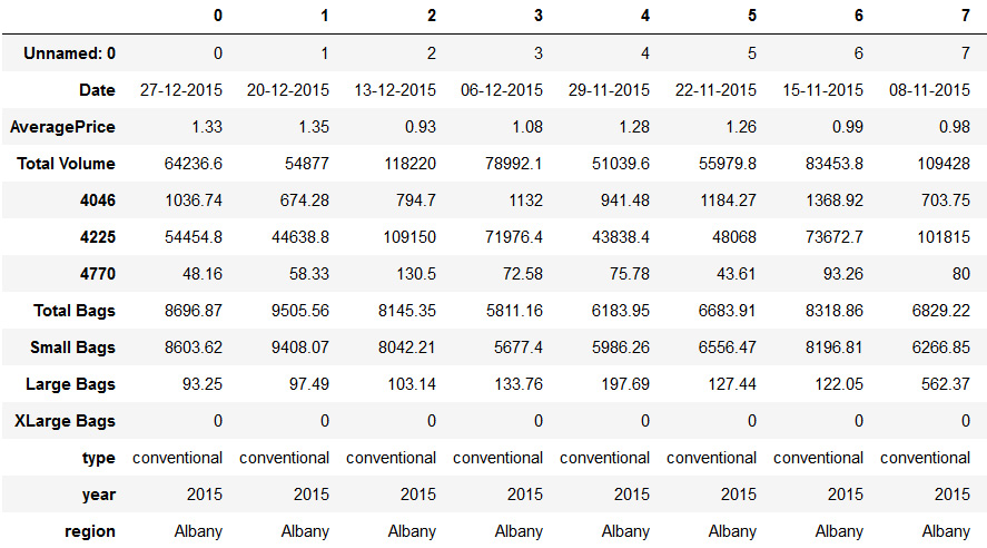
   Figure 5.29: Screenshot showing avocado dataset

2. Look through the data and split the date column into days and months. This will help us catch the seasonality while ignoring the year. Now, drop the date and unnamed columns.

   data['Day'], data['Month'] = data.Date.str[:2], data.Date.str[3:5]

   data = data.drop(['Unnamed: 0', 'Date'], axis = 1)

3. Encode the categorical variables using the LabelEncoder so that Keras can use it to train the model.

   from sklearn.preprocessing import LabelEncoder

   from collections import defaultdict

   label_dict = defaultdict(LabelEncoder)

   data[['region', 'type', 'Day', 'Month', 'year']] = data[['region', 'type', 'Day', 'Month', 'year']].apply(lambda x: label_dict[x.name].fit_transform(x))

4. Split the data into training and testing sets.

   from sklearn.model_selection import train_test_split

   X = data

   y = X.pop('AveragePrice')

   X_train, X_test, y_train, y_test = train_test_split(X, y, test_size=0.3, random_state=9)

5. Use callbacks to save the model whenever the loss improves and for early stopping of the model if it starts performing poorly.

   from keras.callbacks import ModelCheckpoint, EarlyStopping

   filepath="avocado-{epoch:02d}-{val_loss:.2f}.hdf5"

   model_ckpt = ModelCheckpoint(filepath, monitor='val_loss', verbose=1, save_best_only=True, mode='auto')

   es = EarlyStopping(monitor='val_loss', min_delta=1, patience=5, verbose=1)

   callbacks = [model_ckpt, es]

6. Create a neural network model. Here, we make use of the same model as before.

   from keras.models import Sequential

   from keras.layers import Dense

   model = Sequential()

   model.add(Dense(units=16, activation='relu', input_dim=13))

   model.add(Dense(units=8, activation='relu'))

   model.add(Dense(units=1, activation='linear'))

   model.compile(loss='mse', optimizer='adam')

7. Train and evaluate the model to get the MSE of the model.

   model.fit(X_train, y_train, validation_data = (X_test, y_test), epochs=40, batch_size=32)

   model.evaluate(X_test, y_test)

8. Check the final output in the following screenshot:

Figure 5.30: MSE of model

Congratulations! You have just trained your neural network to get a reasonable error on the avocado dataset. The value shown above is the mean square error of the model. Modify some hyperparameters and use the rest of the data to see if you can get a better error score. Make use of the information provided in the previous sections.

Note

A decrease in MSE is favorable. The most optimal value will depend on the situation. For example, while predicting the speed of a car, values less than 100 are ideal, whereas when predicting the GDP of a country, an MSE of 1000 is good enough.

Categorical Variables

A categorical variable is one whose values can be represented in different categories. Examples are colours of a ball, breed of dogs, and zip codes. Mapping these categorical variables in a single dimension creates a sort of dependence on each other, which is incorrect. Even though these categorical variables do not have an order or dependence, inputting them to a neural network as a single feature makes the neural network create dependence between these variables depending on the order, whereas in reality, the order does not mean anything. In this section, we will learn about the ways in which can fix this issue and train effective models.

One-hot Encoding

The easiest and the most widely used method of mapping categorical variables is to use one-hot encoding. Using this method, we convert a categorical feature into features equal to the number of categories in the feature.

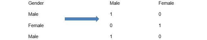
Figure 5.31: Categorical feature conversion

Use the following steps to convert categorical variables into one-hot encoded variables:

1. Convert the data into a number if represented as a data type other than int. There are two ways to do this
2. You can directly use the LabelEncoder method of sklearn.
3. Create bins to reduce the number of categories. The higher the number of categories, the more difficult it is for the model. You can choose an integer to represent each bin. Do keep in mind that doing this will lead to a loss in information and might result in a bad model. You can perform histogram binning using the following rule:

   If the number of categorical columns is less than 25, use 5 bins.

   If it is between 25 and 100, use n/5 bins, where n is the number of categorical columns, and if it is more than 100, use 10 * log (n) bins.

   Note

   You can combine the categories with frequencies smaller than 5% into one category.

4. Convert the numerical array from Step 1 into a one-hot vector using the get_dummies function of pandas.

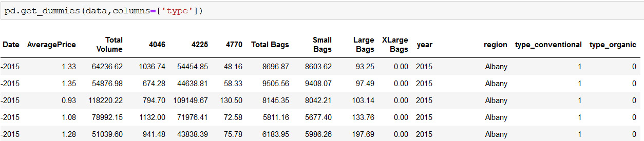
Figure 5.32: Output of get_dummies function

There are two main reasons why one-hot encoding isn't the best way to use categorical data:

• Different values of the categorical variables are assumed to be completely independent of each other. This leads to a loss of information about the relationship between them.
• Categorical variables with many categories result in a very computationally expensive model. Wider datasets require more data points to make meaningful models. This is known as the curse of dimensionality.

To work through these issues, we will use entity embedding.

Entity Embedding

Entity embedding represents categorical features in a multidimensional space. This ensures that the network learns the correct relationship between the different categories of a feature. The dimensions of this multidimensional space do not represent anything specific; it could be anything that the model deems fit to learn. For example, in the case of the days of a week, one dimension could be whether the day is a weekday or not and another could be the distance from a weekday. This method has been inspired from word embedding that is used in natural language processing to learn the semantic similarities between words and phrases. Creating an embedding can help teach the neural networks how Friday is different from Wednesday or how a puppy and a dog are different. For example, a four-dimensional embedding matrix for the days of the week will look something like this:

Figure 5.33: Four-dimensional embedding matrix

From the above matrix, you can see that the embedding learns the dependence between the categories: it knows that Saturday and Sunday are more similar than Thursday and Friday, as the vectors for Saturday and Sunday are similar. Entity embedding gives a big edge when you have a lot of categorical variables in your dataset. To create entity embedding in Keras, you can use the embedding layer.

Note

Always try to use word embedding as it gives the best result.

Exercise 49: Predicting Avocado Price Using Entity Embedding

Let us use the knowledge of entity embedding to predict the avocado price by creating a better neural network model. We will use the same avocado dataset from before.

1. Import the avocado price dataset and check for null values. Split the date column into month and day columns.

   import pandas as pd

   import numpy as np

   data = pd.read_csv('data/avocado.csv')

   data['Day'], data['Month'] = data.Date.str[:2], data.Date.str[3:5]

   data = data.drop(['Unnamed: 0', 'Date'], axis = 1)

   data = data.dropna()

2. Encode the categorical variables.

   from sklearn.preprocessing import LabelEncoder

   from collections import defaultdict

   label_dict = defaultdict(LabelEncoder)

   data[['region', 'type', 'Day', 'Month', 'year']] = data[['region', 'type', 'Day', 'Month', 'year']].apply(lambda x: label_dict[x.name].fit_transform(x))

3. Split the data into training and testing sets.

   from sklearn.model_selection import train_test_split

   X = data

   y = X.pop('AveragePrice')

   X_train, X_test, y_train, y_test = train_test_split(X, y, test_size=0.3, random_state=9)

4. Create a dictionary that maps categorical column names to the unique values in them.

   cat_cols_dict = {col: list(data[col].unique()) for col in ['region', 'type', 'Day', 'Month', 'year'] }

5. Next, get the input data in the format that the embedding neural network will accept.

   train_input_list = []

   test_input_list = []

   for col in cat_cols_dict.keys():

       raw_values = np.unique(data[col])

       value_map = {}

       for i in range(len(raw_values)):

           value_map[raw_values[i]] = i

       train_input_list.append(X_train[col].map(value_map).values)

       test_input_list.append(X_test[col].map(value_map).fillna(0).values)

   other_cols = [col for col in data.columns if (not col in cat_cols_dict.keys())]

   train_input_list.append(X_train[other_cols].values)

   test_input_list.append(X_test[other_cols].values)

   Here, what we are doing is creating a list of arrays of all the variables.

6. Next, create a dictionary that will store the output dimensions of the embedding layers. This is the number of values the variable will be denoted by. You must get to the right number with trial and error.

   cols_out_dict = {

       'region': 12,

       'type': 1,

       'Day': 10,

       'Month': 3,

       'year': 1

   }

7. Now, create the embedding layers for the categorical variables. In each iteration of the loop, we create one embedding layer for the categorical variable.

   from keras.models import Model

   from keras.layers import Input, Dense, Concatenate, Reshape, Dropout

   from keras.layers.embeddings import Embedding

   inputs = []

   embeddings = []

   for col in cat_cols_dict.keys():

       

       inp = Input(shape=(1,), name = 'input_' + col)

       embedding = Embedding(cat_cols_dict[col], cols_out_dict[col], input_length=1, name = 'embedding_' + col)(inp)

       embedding = Reshape(target_shape=(cols_out_dict[col],))(embedding)

       inputs.append(inp)

       embeddings.append(embedding)

8. Now, add the continuous variable to the network and complete the model.

   input_numeric = Input(shape=(8,))

   embedding_numeric = Dense(16)(input_numeric)

   inputs.append(input_numeric)

   embeddings.append(embedding_numeric)

   x = Concatenate()(embeddings)

   x = Dense(16, activation='relu')(x)

   x = Dense(4, activation='relu')(x)

   output = Dense(1, activation='linear')(x)

   model = Model(inputs, output)

   model.compile(loss='mse', optimizer='adam')

9. Train the model with the train_input_list, which we created in Step 5 for 50 epochs.

   model.fit(train_input_list, y_train, validation_data = (test_input_list, y_test), epochs=50, batch_size=32)

10. Now, get the weights from the embedding layers to visualize the embedding.

    embedding_region = model.get_layer('embedding_region').get_weights()[0]

11. Perform PCA and plot the output using the region labels (which you can get by performing inverse transform on the dictionary that we created earlier). PCA displays similar data points closer, by reducing the dimensionality to two dimensions. Here, we plot only the first 25 regions.

    You can plot all of them if you want.

    import matplotlib.pyplot as plt

    from sklearn.decomposition import PCA

    pca = PCA(n_components=2)

    Y = pca.fit_transform(embedding_region[:25])

    plt.figure(figsize=(8,8))

    plt.scatter(-Y[:, 0], -Y[:, 1])

    for i, txt in enumerate((label_dict['region'].inverse_transform(cat_cols_dict['region']))[:25]):

        plt.annotate(txt, (-Y[i, 0],-Y[i, 1]), xytext = (-20, 8), textcoords = 'offset points')

    plt.show()

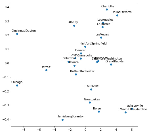
Figure 5.34: Graphical representation of avocado growing region using entity embedding

Congratulations! You improved the accuracy of your model by using entity embedding. As you can see from the embedding plot, the model was able to figure out the regions with high and low average prices. You can plot the embedding of other variables to see what relationships the network makes from the data. Also, try to improve the accuracy of this model through hyperparameter tuning.

Activity 16: Predicting a Customer's Purchase Amount

In this activity, we will attempt to predict the amount a customer will spend on a product category. The dataset (https://github.com/TrainingByPackt/Data-Science-with-Python/tree/master/Chapter05/data) contains transactions made in a retail store. Let's look at the following scenario: You work at a big retail chain and want to predict which kind of customer will spend how much money on a particular product category. Doing this will help your frontline staff recommend the right kind of products to customers, thus increasing sales and customer satisfaction. To do this, you need to create a machine learning model that predicts the purchase value of a transaction.

1. Load the Black Friday dataset using pandas. This dataset is a collection of transactions made in a retail store. The information it contains is the age, city, marital status of the customer, product category of the item being bought, and bill amount. The first few rows should look like this:
   

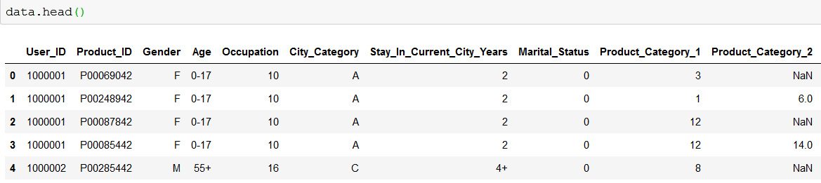
   Figure 5.35: Screenshot showing first five elements of Black Friday dataset

   Remove unnecessary variables and null values. Remove Product_Category_2 and Product_Category_3 columns.

2. Encode all the categorical variables.
3. Perform prediction by creating a neural network with the Keras library. Make use of entity embedding and perform hyperparameter tuning.
4. Save your model for future use.

   Note

   The solution for this activity can be found on page 364.

Summary

In this chapter, we learnt how to create highly accurate structured data models and understood what XGBoost is and how to use the library to train models, Before we started, we were wondering what neural networks are and how to use the Keras library to train models. After learning about neural networks, we moved to handling categorical data. Finally, we learned what cross-validation is and how to use it.

Now that you have completed this chapter, you can handle any kind of structured data and creating machine learning models with it. In the next chapter, you will learn how to create neural network models for image data.