Chapter 6

Decoding Images

Learning Objectives

By the end of this chapter, you will be able to:

• Create models that can classify images into different categories
• Use the Keras library to train neural network models for images
• Utilize concepts of image augmentation in different business scenarios
• Extract meaningful information from images

This chapter will cover various concepts on how to read and process images.

Introduction

So far, we have only been working with numbers and text. In this chapter, we will learn how to use machine learning to decode images and extract meaningful information, such as the type of object present in an image, or the number written in an image. Have you ever stopped to think about how our brains interpret the images they receive from our eyes? After millions of years of evolution, our brains have become highly efficient and accurate at recognizing objects and patterns from the images they get from our eyes. We have been able to replicate the function of our eyes using cameras, but making computers recognize patterns and objects in images is a really tough job. The field associated with understanding what is present in images is known as computer vision. The field of computer vision has witnessed tremendous research and advancements in the past few years. The introduction of Convoluted Neural Networks (CNNs) and the ability to train neural networks on GPUs were the biggest of these breakthroughs. Today, CNNs are used anywhere we have a computer vision problem, for example, self-driving cars, facial recognition, object detection, object tracking, and creating fully autonomous robots. In this chapter, we will learn how these CNNs work and how big an improvement they are compared to traditional methods.

Images

The digital cameras that we have today store images as a big matrix of numbers. These are what we call digital images. A single number on this matrix refers to a single pixel in the image. Individual numbers refer to the intensity of the color at that pixel. For a grayscale image, these values vary from 0 to 255, where 0 is black and 255 is white. For a colored image, this matrix is three-dimensional, where each dimension has values for red, green, and blue. The values in the matrices refer to the intensities of the respective colors. We use these values as input to our computer vision programs or data science models to perform predictions and recognitions.

Now, there are two ways for us to create machine learning models using these pixels:

• Input individual pixels as different input variables to the neural network
• Use a convolutional neural network

Creating a fully connected neural network that takes individual pixel values as input variables is the easiest and the most intuitive way for us right now, so we will start by creating this model. In the next section, we will learn about CNNs and see how much better they are at dealing with images.

Exercise 50: Classify MNIST Using a Fully Connected Neural Network

In this exercise, we will perform classification on the Modified National Institute of Standards and Technology database (MNIST) dataset. MNIST is a dataset of handwritten digits that have been normalized to fit into a 28 x 28 pixel bounding box. There are 60,000 training images and 10,000 testing images in this dataset. In case of the fully connected network, we feed the individual pixels as features to the network, and then train it as a normal neural network, much like the first neural network we trained in Chapter 5, Mastering Structured Data.

To complete this exercise, complete the following steps:

1. Load the required libraries, as illustrated here:

   import numpy as np

   import matplotlib.pyplot as plt

   from sklearn.preprocessing import LabelBinarizer

   from keras.datasets import mnist

   from keras.models import Sequential

   from keras.layers import Dense

2. Load the MNIST dataset using the Keras library:

   (x_train, y_train), (x_test, y_test) = mnist.load_data()

3. From the shape of the dataset, you can figure out that the data is available in 2D format. The first element is the number of images available, whereas the next two elements are the width and height of the images:

   x_train.shape

   The output is as follows:

   

   Figure 6.1: Width and height of images

4. Plot the first image to see what kind of data you are dealing with:

   plt.imshow(x_test[0], cmap=plt.get_cmap(‘gray'))

   plt.show()

   

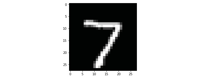
   Figure 6.2: Sample image of the MNIST dataset

5. Convert the 2D data into 1D data so that our neural network can take it as input (28 x 28 pixels = 784):

   x_train = x_train.reshape(60000, 784)

   x_test = x_test.reshape(10000, 784)

6. Convert the target variable to a one-hot vector so that our network does not form unnecessary connections between the different target variables:

   label_binarizer = LabelBinarizer()

   label_binarizer.fit(range(10))

   y_train = label_binarizer.transform(y_train)

   y_test = label_binarizer.transform(y_test)

7. Create the model. Make a small two-layer network; you can experiment with other architectures. You will learn more about cross-entropy loss in the following section:

   model = Sequential()

   model.add(Dense(units=32, activation='relu', input_dim=784))

   model.add(Dense(units=32, activation='relu'))

   model.add(Dense(units=10, activation='softmax'))

   model.compile(loss='categorical_crossentropy', optimizer='adam', metrics = [‘acc'])

   model.summary()

   

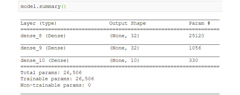
   Figure 6.3: Model architecture of the dense network

8. Train the model and check the final accuracy:

   model.fit(x_train, y_train, validation_data = (x_test, y_test), epochs=40, batch_size=32)

   score = model.evaluate(x_test, y_test)

   print(“Accuracy: {0:.2f}%”.format(score[1]*100))

   The output is as follows:

Figure 6.4: Model accuracy

Congratulations! You have now created a model that can predict the number on an image with 93.57% accuracy. You can plot different test images and see your network's result using the following code. Change the value of the image variable to get different images:

image = 6

plt.imshow(x_test[image].reshape(28,28),

cmap=plt.get_cmap(‘gray'))

plt.show()

y_pred = model.predict(x_test)

print(“Prediction: {0}”.format(np.argmax(y_pred[image])))

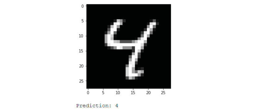
Figure 6.5: An MNIST image with prediction from dense network

You can visualize only the incorrect predictions to understand where your model fails:

incorrect_indices = np.nonzero(np.argmax(y_pred,axis=1) != np.argmax(y_test,axis=1))[0]

image = 4

plt.imshow(x_test[incorrect_indices[image]].reshape(28,28),

cmap=plt.get_cmap(‘gray'))

plt.show()

print(“Prediction: {0}”.format(np.argmax(y_pred[incorrect_indices[image]])))

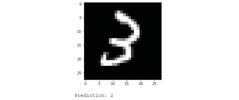
Figure 6.6: Incorrectly classified example from the dense network

As you can see in the previous screenshot, the model failed because we predicted the class to be 2 whereas the correct class was 3.

Convolutional Neural Networks

Convolutional Neural Network (CNN) is the name given to a neural network that has convolutional layers. These convolutional layers handle the high dimensionality of raw images efficiently with the help of convolutional filters. CNNs allow us to recognize highly complex patterns in images, which would be impossible with a simple neural network. CNNs can also be used for natural language processing.

The first few layers of a CNN are convolutional, where the network applies different filters to the image to find useful patterns in the image; then there's the pooling layers, which help down-sample the output of the convolutional layers. The activation layer controls which signal flows from one layer to the next, emulating the neurons in our brain. The last few layers in the network are dense layers; these are the same layers we used for the previous exercise.

Convolutional Layer

The convolutional layer consists of multiple filters that learn to activate when they see a certain feature, edge, or color in the initial layers, and eventually faces, honeycombs, and wheels. These filters are exactly like the Instagram filters that we are all so used to. Filters change the appearance of the image by altering the pixels in a certain manner. Let's take a filter that detects horizontal edges as an example.

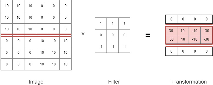
Figure 6.7: Horizontal edge detection filter

As you can see in the preceding screenshot, the filter transforms the image into another image that has the horizontal line highlighted. To get the transformation, we multiply parts of the image by the filter one by one. First, we take the top-left 3 x 3 cross section of the image and perform matrix multiplication with the filter to get the first top-left pixel of the transformation. Then we move the filter one pixel to the right and get the second pixel of the transformation, and so on. The transformation is a new image that has only the horizontal line section of the image highlighted. The values of the filter parameters, 9 in this case, are the weights or parameters that a convolutional layer learns while training. Some filters might learn to detect horizontal lines, some vertical lines, and some lines at a 45-degree angle. The subsequent layers learn more complex structures, such as the pattern of a wheel or a human face.

Some hyperparameters of the convolutional layer are listed here:

• Filters: This is the count of filters in each layer of the network. This number also reflects the dimension of the transformation, because each filter will result in one dimension of the output.
• Filter size: This is the size of the convolutional filter that the network will learn. This hyperparameter will determine the size of the output transformation.
• Stride: In the preceding horizontal edge example, we moved the filter by one pixel every pass. This is the stride. It refers to how much the filter will move every pass. This hyperparameter also determines the size of the output transformation.
• Padding: This hyperparameter makes the network pad the image with zeros on all the sides. This helps preserve edge information in some cases and helps us keep the input and output of the same size.

  Note

  If you perform padding, then you get an image of the same or larger size as the output of the convolution operation. If you do not perform padding, then the image will decrease in size.

Pooling Layer

Pooling layers reduce the size of the input image to reduce the amount of computation and parameters in the network. Pooling layers are inserted periodically between convolutional layers to control overfitting. The most common variant of pooling is 2 x 2 max pooling with a stride of 2. This variant performs down-sampling of the input to keep only the maximum value of the four pixels in the output. The depth dimension remains unchanged.

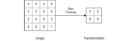
Figure 6.8: Max pooling operation

in the past, we used to perform average pooling as well, but max pooling is used more often nowadays because it has proven to work better in practice. Many data scientists do not like using pooling layers, simply due to the information loss that accompanies the pooling operation. There has been some research on this topic, and it has been found that simple architectures without pooling layers outperform state-of-the-art models at times. To reduce the size of the input, it is suggested to use larger strides in the convolutional layer every once in a while.

Note

The research paper Striving for Simplicity: The All Convolutional Net evaluates models with pooling layers to find that pooling layers do not always improve the performance of the network, mostly when enough data is available. For more information, read the Striving for Simplicity: The All Convolutional Net paper: https://arxiv.org/abs/1412.6806

Adam Optimizer

Optimizers update weights with the help of loss functions. Selecting the wrong optimizer or the wrong hyperparameter for the optimizer can lead to a delay in finding the optimal solution for the problem.

The name Adam is derived from adaptive moment estimation. Adam has been designed specifically for training deep neural networks. The use of Adam is widespread in the data science community due to its speed in getting close to the optimal solution. Thus, if you want fast convergence, use the Adam optimizer. Adam does not always lead to the optimal solution; in such cases, SGD with momentum helps achieve state-of-the-art results. The following would be the parameters:

• Learning rate: This is the step size for the optimizer. Larger values (0.2) result in faster initial learning, whereas smaller values (0.00001) slow the learning down during training.
• Beta 1: This is the exponential decay rate for the mean estimates of the gradient.
• Beta 2: This is the exponential decay rate for the uncentered variance estimates of the gradient.
• Epsilon: This is a very small number to prevent division by zero.

A good starting point for deep learning problems are learning rate = 0.001, beta 1 = 0.9, beta 2 = 0.999, and epsilon = 10-8.

Note

For more information, read the Adam paper: https://arxiv.org/abs/1412.6980v8

Cross-entropy Loss

Cross-entropy loss is used when we are working with a classification problem where the output of each class is a probability value between 0 and 1. The loss here increases as the model deviates from the actual value; it follows a negative log graph. This helps when the model predicts probabilities that are far from the actual value. For example, if the probability of the true label is 0.05, we penalize the model with a huge loss. On the other hand, if the probability of the true label is 0.40, we penalize it with a smaller loss.

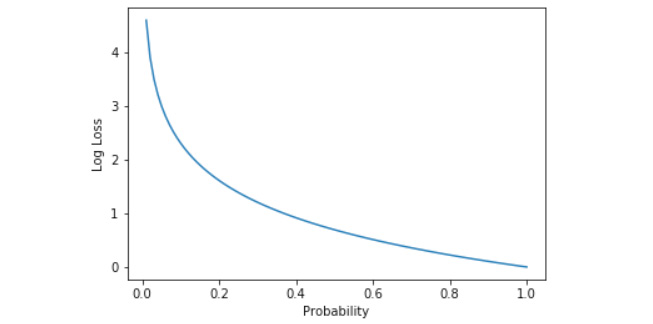
Figure 6.9: Graph of log loss versus probability

The preceding graph shows that the loss increases exponentially as the predictions get further from the true label. The formula that the cross-entropy loss follows is as follows:

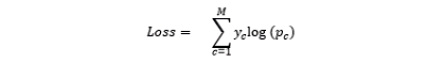
Figure 6.10: Cross entropy loss formula

M is number of classes in the dataset (10 in the case of MNIST), y is the true label, and p is the predicted probability of the class. We prefer cross-entropy loss for classification since the weight update becomes smaller as we get closer to the ground truth. Cross-entropy loss penalizes the probability of the correct class only.

Exercise 51: Classify MNIST Using a CNN

In this exercise, we will perform classification on the Modified National Institute of Standards and Technology (MNIST) dataset using a CNN instead of the fully connected layers used in Exercise 50. We feed the network the complete image as input and get the number on the image as output:

1. Load the MNIST dataset using the Keras library:

   from keras.datasets import mnist

   (x_train, y_train), (x_test, y_test) = mnist.load_data()

2. Convert the 2D data into 3D data with the third dimension having only one layer, which is how Keras requires the input:

   x_train = x_train.reshape(-1, 28, 28, 1)

   x_test = x_test.reshape(-1, 28, 28, 1)

3. Convert the target variable to a one-hot vector so that our network does not form an unnecessary connection between the different target variables:

   from sklearn.preprocessing import LabelBinarizer

   label_binarizer = LabelBinarizer()

   label_binarizer.fit(range(10))

   y_train = label_binarizer.transform(y_train)

   y_test = label_binarizer.transform(y_test)

4. Create the model. Here, we make a small CNN. You can experiment with other architectures:

   from keras.models import Model, Sequential

   from keras.layers import Dense, Conv2D, MaxPool2D, Flatten

   model = Sequential()

   Add the convolutional layers:

   model.add(Conv2D(32, kernel_size=3,

   padding=”same”,input_shape=(28, 28, 1), activation = ‘relu'))

   model.add(Conv2D(32, kernel_size=3, activation = ‘relu'))

   Add the pooling layer:

   model.add(MaxPool2D(pool_size=(2, 2)))

5. Flatten the 2D matrices into 1D vectors:

   model.add(Flatten())

6. Use dense layers as the final layers for the model:

   model.add(Dense(128, activation = “relu”))

   model.add(Dense(10, activation = “softmax”))

   model.compile(loss='categorical_crossentropy', optimizer='adam',

   metrics = [‘acc'])

   model.summary()

   To understand this fully, look at the output of the model in the following screenshot:

   

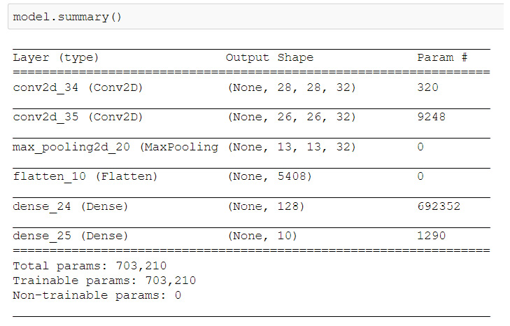
   Figure 6.11: Model architecture of the CNN

7. Train the model and check the final accuracy:

   model.fit(x_train, y_train, validation_data = (x_test, y_test),

   epochs=10, batch_size=1024)

   score = model.evaluate(x_test, y_test)

   print(“Accuracy: {0:.2f}%”.format(score[1]*100))

   The output is as follows:

Figure 6.12: Final model accuracy

Congratulations! You have now created a model that can predict the number on an image with 98.62% accuracy. You can plot different test images and see your network's result using the code given in Exercise 50. Also, plot the incorrect predictions to see where the model went wrong:

import numpy as np

import matplotlib.pyplot as plt

incorrect_indices = np.nonzero(np.argmax(y_pred,axis=1) != np.argmax(y_test,axis=1))[0]

image = 4

plt.imshow(x_test[incorrect_indices[image]].reshape(28,28),

cmap=plt.get_cmap(‘gray'))

plt.show()

print(“Prediction: {0}”.format(np.argmax(y_pred[incorrect_indices[image]])))

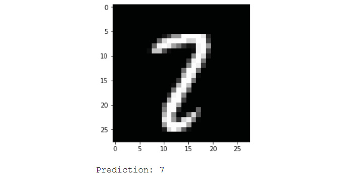
Figure 6.13: Incorrect prediction of the model; the true label is 2

As you can see, the model is having difficulty predicting images that are ambiguous. You can play around with the layers and hyperparameters to see if you can get a better accuracy. Try substituting the pooling layers with convolutional layers with a higher stride, as suggested in the previous section.

Regularization

Regularization is a technique that helps machine learning models generalize better by making modifications in the learning algorithm. This helps prevent overfitting and helps our model work better on data that it hasn't seen during training. In this section, we will learn about the different regularizers available to us.

Dropout Layer

Dropout is a regularization technique that we use to prevent overfitting in our neural network models. We ignore randomly selected neurons from the network while training. This prevents the activations of those neurons continuing down the line, and the weight updates are not applied to them during back propagation. The weights of neurons are tuned to identify specific features; neurons that neighbor them become dependent on this, which can lead to overfitting because these neurons can get specialized to the training data. When neurons are randomly dropped, the neighboring neurons step in and learn the representation, leading to multiple different representations being learned by the network. This make the network generalize better and prevents the model from overfitting. One import thing to keep in mind is that dropout layers should not be used when you are performing predictions or testing your model. This would make the model lose valuable information and would lead to a loss in performance. Keras takes care of this by itself.

When using the dropout layer, it is recommended to create larger networks because it gives the model more opportunities to learn. We generally use a dropout probability between 0.2 and 0.5. This probability refers to the probability by which a neuron will be dropped from training. A dropout layer after every layer is found to give good results, so you can start by placing dropout layers with a probability of 0.2 after every layer and then fine-tune from there.

To create a dropout layer in Keras with a probability of 0.5, you can use the following function:

keras.layers.Dropout(0.5)

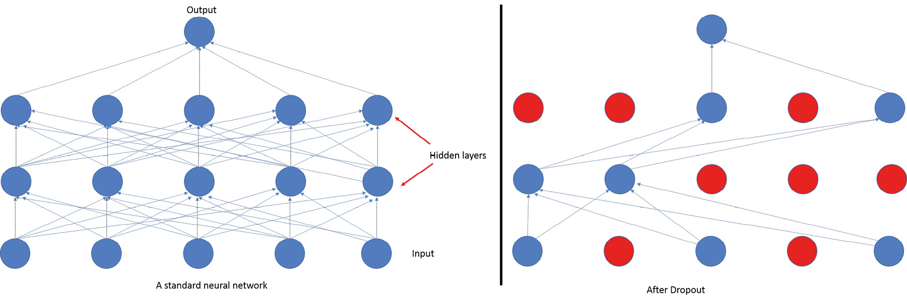
Figure 6.14: Visualizing dropout in a dense neural network

L1 and L2 Regularization

L2 is the most common type of regularization, followed by L1. These regularizers work by adding a term to the loss of the model to get the final cost function. This added term leads to a decrease in the weights of the model. This in turn leads to a model that generalizes well.

The cost function of L1 regularization looks like this:

Figure 6.15: Cost function of L1 regularization

Here, λ is the regularization parameter. L1 regularization leads to weights that are very close to zero. This makes the neurons with L1 regularization become dependent only on the most important inputs and ignore the noisy inputs.

The cost function of L2 regularization looks like this:

Figure 6.16: Cost function of L2 regularization

L2 regularization heavily penalizes high-weight vectors and prefers weights that are diffused. L2 regularization is also known as weight decay because it forces the weights of a network to decay towards zero but, unlike L1 regularization, not exactly to zero. We can combine L1 and L2 and implement them together. To implement these regularizers, you can use the following functions in Keras:

keras.regularizers.l1(0.01)

keras.regularizers.l2(0.01)

keras.regularizers.l1_l2(l1=0.01, l2=0.01)

Batch Normalization

In Chapter 1, Introduction to Data Science and Data Pre processing we learned how to perform normalization and how it helped speed up the training of our machine learning models. Here, we will extend that same normalization to the individual layers of the neural network. Batch normalization allows layers to learn independently of other layers. It does this by normalizing the inputs to a layer to have a fixed mean and variance; this prevents the changes in parameters of previous layers from affecting the input of the layer too much. It also has a slight regularization effect; much like dropout, it prevents overfitting, but it does that by introducing noise into the values of the mini batches. When using batch normalization, make sure to use a lower dropout, which is better because dropout leads to a loss of information. However, do not remove dropout and rely completely on batch normalization, because a combination of the two has been seen to work better. While using batch normalization, a higher learning rate can be used because it makes sure that no action is too high or too low.

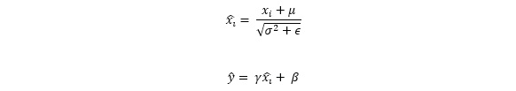
Figure 6.17: Batch normalization equation

Here, (xi) is the input to the layer and y is the normalized input. μ is the batch mean and σ2 is the batch's standard deviation. Batch normalization introduces two new (x_i ) ̂the loss.

To create a batch normalization layer in Keras, you can use the following function:

keras.layers.BatchNormalization()

Exercise 52: Improving Image Classification Using Regularization Using CIFAR-10 images

In this exercise, we will perform classification on the Canadian Institute for Advanced Research (CIFAR-10) dataset. It consists of 60,000 32 x 32 color images in 10 classes. The 10 different classes represent birds, airplanes, cats, cars, frogs, deer, dogs, trucks, ships, and horses. It is one of the most widely used datasets for machine learning research, mainly in the field of CNNs. Due to the low resolution of the images, models can be trained much quicker on these images. We will use this dataset to implement some of the regularization techniques we learned in the previous section:

Note

To get the raw CIFAR-10 files and CIFAR-100 dataset, visit https://www.cs.toronto.edu/~kriz/cifar.html.

1. Load the CIFAR-10 dataset using the Keras library:

   from keras.layers import Dense, Conv2D, MaxPool2D, Flatten, Dropout, BatchNormalization

   from keras.datasets import cifar10

   (x_train, y_train), (x_test, y_test) = cifar10.load_data()

2. Check the dimensions of the data:

   x_train.shape

   The output is as follows:

   

   Figure 6.18: Dimensions of x

   Similar dimensions, for y:

   y_train.shape

   The output is as follows:

   

   Figure 6.19: Dimensions of y

   As these are color images, they have three channels.

3. Convert the data to the format that Keras requires:

   x_train = x_train.reshape(-1, 32, 32, 3)

   x_test = x_test.reshape(-1, 32, 32, 3)

4. Convert the target variable to a one-hot vector so that our network does not form unnecessary connections between the different target variables:

   from sklearn.preprocessing import LabelBinarizer

   label_binarizer = LabelBinarizer()

   label_binarizer.fit(range(10))

   y_train = label_binarizer.transform(y_train)

   y_test = label_binarizer.transform(y_test)

5. Create the model. Here, we make a small CNN without regularization first:

   from keras.models import Sequential

   model = Sequential()

   Add the convolutional layers:

   model.add(Conv2D(32, (3, 3), activation='relu', padding='same', input_shape=(32,32,3)))

   model.add(Conv2D(32, (3, 3), activation='relu'))

   Add the pooling layer:

   model.add(MaxPool2D(pool_size=(2, 2)))

6. Flatten the 2D matrices into 1D vectors:

   model.add(Flatten())

7. Use dense layers as the final layers for the model and compile the model:

   model.add(Dense(512, activation='relu'))

   model.add(Dense(10, activation='softmax'))

   model.compile(loss='categorical_crossentropy', optimizer='adam',

   metrics = [‘acc'])

8. Train the model and check the final accuracy:

   model.fit(x_train, y_train, validation_data = (x_test, y_test),

   epochs=10, batch_size=512)

9. Now check the accuracy of the model:

   score = model.evaluate(x_test, y_test)

   print(“Accuracy: {0:.2f}%”.format(score[1]*100))

   The output is as follows:

   

   Figure 6.20: Accuracy of model

10. Now create the same model, but with regularization. You can experiment with other architectures as well:

    model = Sequential()

    Add the convolutional layers:

    model.add(Conv2D(32, (3, 3), activation='relu', padding='same', input_shape=(32,32,3)))

    model.add(Conv2D(32, (3, 3), activation='relu'))

    Add the pooling layer:

    model.add(MaxPool2D(pool_size=(2, 2)))

11. Add the batch normalization layer along with a dropout layer:

    model.add(BatchNormalization())

    model.add(Dropout(0.10))

12. Flatten the 2D matrices into 1D vectors:

    model.add(Flatten())

13. Use dense layers as the final layers for the model and compile the model:

    model.add(Dense(512, activation='relu'))

    model.add(Dropout(0.5))

    model.add(Dense(10, activation='softmax'))

    model.compile(loss='categorical_crossentropy', optimizer='adam',

    metrics = [‘acc'])

    model.summary()

    

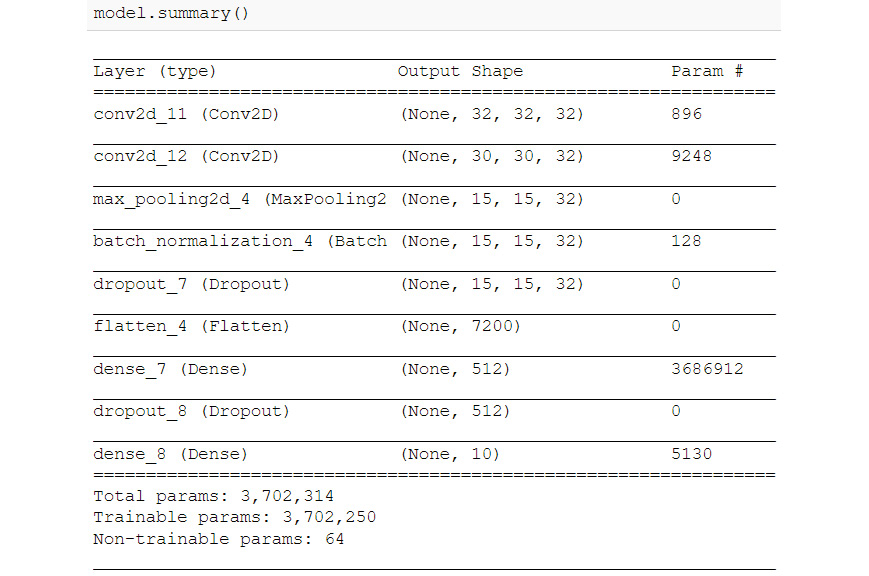
    Figure 6.21: Architecture of the CNN with regularization

14. Train the model and check the final accuracy:

    model.fit(x_train, y_train, validation_data = (x_test, y_test),

    epochs=10, batch_size=512)

    score = model.evaluate(x_test, y_test)

    print(“Accuracy: {0:.2f}%”.format(score[1]*100))

    The output is as follows:

Figure 6.22: Final accuracy output

Congratulations! You made use of regularization to make your model work better than before. If you do not see an improvement in your model, train it for longer, so set it for more epochs. You will also see that you can train for a lot more epochs without worrying about overfitting.

You can plot different test images and see your network's result using the code given in Exercise 50. Also, plot the incorrect predictions to see where the model went wrong:

import numpy as np

import matplotlib.pyplot as plt

y_pred = model.predict(x_test)

incorrect_indices = np.nonzero(np.argmax(y_pred,axis=1) != np.argmax(y_test,axis=1))[0]

labels = [‘airplane', ‘automobile', ‘bird', ‘cat', ‘deer', ‘dog', ‘frog', ‘horse', ‘ship', ‘truck']

image = 3

plt.imshow(x_test[incorrect_indices[image]].reshape(32,32,3))

plt.show()

print(“Prediction: {0}”.format(labels[np.argmax(y_pred[incorrect_indices[image]])]))

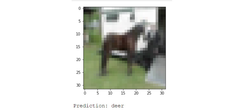
Figure 6.23: Incorrect prediction of the model

As you can see, the model is having difficulty in predicting images that are ambiguous. The true label is horse. You can play around with the layers and hyperparameters to see if you can get a better accuracy. Try creating more complex models with regularization and train them for longer.

Image Data Preprocessing

In this section, we go over a few techniques that you can use as a data scientist to preprocess images. First, we look at image normalization, and then we learn how we can convert a color image into a greyscale image. Finally, we look at ways in which we can bring all images in a dataset to the same dimensions. Preprocessing images is needed because datasets do not contain images that are the same size; we need to convert them into a standard size to train machine learning models on them. Some image preprocessing techniques help by reducing the model's training time by either making the important features easier to identify for the model or by reducing the dimensions as in the case of a greyscale image.

Normalization

In the case of images, the scale of the pixels is of the same order and in the range 0 to 255. Therefore, this normalization step is optional, but it might help speed up the learning process. To reiterate, centering the data and scaling it to the same order helps the network by ensuring that the gradients do not go out of control. A neural network shares parameters (neurons). If inputs are not scaled to the same order, it would make it difficult for the network to learn.

Converting to Grayscale

Depending on the kind of dataset and problem you have, you can convert your images from RGB to greyscale. This helps the network work much more quickly because it has a lot fewer parameters to learn. Depending on the type of problem, you might not want to do this because it leads to a loss in information provided by the colors of the image. To convert an RGB image to a grayscale image, use the Pillow library:

from PIL import Image

image = Image.open(‘rgb.png').convert(‘LA')

image.save(‘greyscale.png')

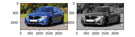
Figure 6.24: Image of a car converted to grayscale

Getting All Images to the Same Size

When working with real-life datasets, you will often come across a major challenge in that not all the images in your dataset will be the same size. You can perform one of the following steps depending on the situation to get around the issue:

• Upsampling: You can upsample smaller images to fix a specific size. If the aspect ratio doesn't match the size that you have decided upon, you can crop the image. There will be some loss of information, but you can get around this by taking different centers while cropping and introducing these new images to the dataset. This will make the model more robust. To do this, utilize the following code:

  from PIL import Image

  img = Image.open(‘img.jpg')

  scale_factor = 1.5

  new_img = img.resize((int(img.size[0]* scale_factor),int(img.size[1]* scale_factor)), Image.BICUBIC)

  The second parameter of the resize function is the algorithm that will be used to get new pixels of the resized image. The bicubic algorithm is fast and is one of the best pixel resampling algorithms for upsampling.

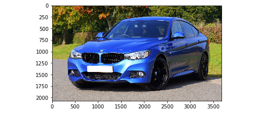
Figure 6.25: Upsampled image of a car

• Downsampling: Similar to upsampling, you can perform downsampling on large images to make then smaller and then crop to fit the size that you have selected. You can use the following code to downsample images:

  scale_factor = 0.5

  new_img = img.resize(

  (int(img.size[0]* scale_factor ),

  int(img.size[1]* scale_factor)),

  Image.ANTIALIAS)

  The second parameter of the resize function is the algorithm that will be used to get the new pixels of the resized image, as mentioned previously. The antialiasing algorithm helps smoothen out the pixelated images. It works better than bicubic but is much slower. Antialiasing is one of the best pixel resampling algorithms for downsampling.

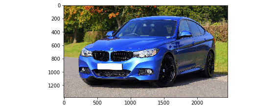
Figure 6.26: Down sampled image of a car

• Crop: This is another method to make all images of the same size is to crop them. As mentioned before, you can use different centers to prevent the loss of information. You can use the following code to crop your images:

  area = (1000, 500, 2500, 2000)

  cropped_img = img.crop(area)

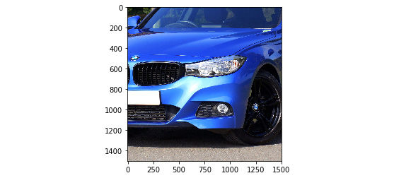
Figure 6.27: Cropped image of a car

• Padding: Padding adds a layer of zeros or ones around the image to increase the size of the image. To perform padding, use the following code:

  size = (2000,2000)

  back = Image.new(“RGB”, size, “white”)

  offset = (250, 250)

  back.paste(cropped_img, offset)

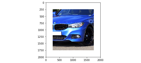
Figure 6.28: Padded image of a cropped car

Other Useful Image Operations

The Pillow library has many functions for modifying and creating new images. These will be helpful for creating new images from our existing training data.

To flip an image, we can use the following code:

img.transpose(Image.FLIP_LEFT_RIGHT)

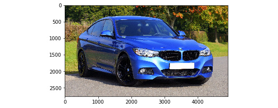
Figure 6.29: Flipped image of a cropped car

To rotate an image by 45 degrees, we can use the following code:

img.rotate(45)

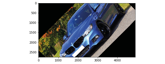
Figure 6.30: The cropped car image rotated 45 degrees

To shift an image by 1,000 pixels, we can use the following code:

import PIL

width, height = img.size

image = PIL.ImageChops.offset(img, 1000, 0)

image.paste((0), (0, 0, 1000, height))

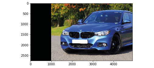
Figure 6.31: Rotated image of the cropped car

Activity 17: Predict if an Image Is of a Cat or a Dog

In this activity, we will attempt to predict if the provided image is of a cat or a dog. The cats and dogs dataset (https://github.com/TrainingByPackt/Data-Science-with-Python/tree/master/Chapter06) from Microsoft contains 25,000 color images of cats and dogs. Let's look at the following scenario: You work at a veterinary clinic with two vets, one that specializes in dogs and one in cats. You want to automate the appointments of the doctors by figuring out if the next client is a dog or a cat. To do this, you create a CNN model:

1. Load the dog versus cat dataset and preprocess the images.
2. Use the image filenames to find the cat or dog label for each image. The first images should look like this:
   

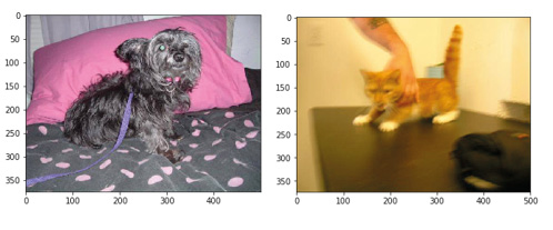
   Figure 6.32: First images of the dog and cat class

3. Get the images in the correct shape to be trained.
4. Create a CNN that makes use of regularization.

   Note

   The solution for this activity can be found on page 369.

You should find that the test set accuracy for this model is 70.4%. The training set accuracy is really high, around 96. This means that the model has started to overfit. Improving the model to get the best possible accuracy is left for you as an exercise. You can plot the incorrectly predicted images using the code from previous exercises to get a sense of how well the model performs:

import matplotlib.pyplot as plt

y_pred = model.predict(x_test)

incorrect_indices = np.nonzero(np.argmax(y_pred,axis=1) != np.argmax(y_test,axis=1))[0]

labels = [‘dog', ‘cat']

image = 5

plt.imshow(x_test[incorrect_indices[image]].reshape(50,50), cmap=plt.get_cmap(‘gray'))

plt.show()

print(“Prediction: {0}”.format(labels[np.argmax(y_pred[incorrect_indices[image]])]))

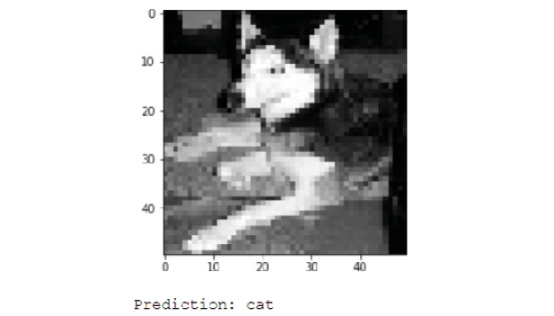
Figure 6.33: Incorrect prediction of a dog by the regularized CNN model

Data Augmentation

While training machine learning models, we data scientists often run into the problem of imbalanced classes and a lack of training data. This leads to sub-par models that perform poorly when deployed in real-life scenarios. One easy way to deal with these problems is data augmentation. There are multiple ways of performing data augmentation, such as rotating the image, shifting the object, cropping an image, shearing to distort the image, and zooming in to a part of the image, as well as more complex methods such as using Generative Adversarial Networks (GANs) to generate new images. GANs are simply two neural networks that are competing with each other. A generator network tries to make images that are similar to the already existing images, while a discriminator network tries to determine if the image was generated or was part of the original data. After the training is complete, the generator network is able to create images that are not a part of the original data but are so similar that they can be mistaken for images that were actually captured by a camera.

Note

You can learn more about GANs in this paper: https://arxiv.org/abs/1406.2661.

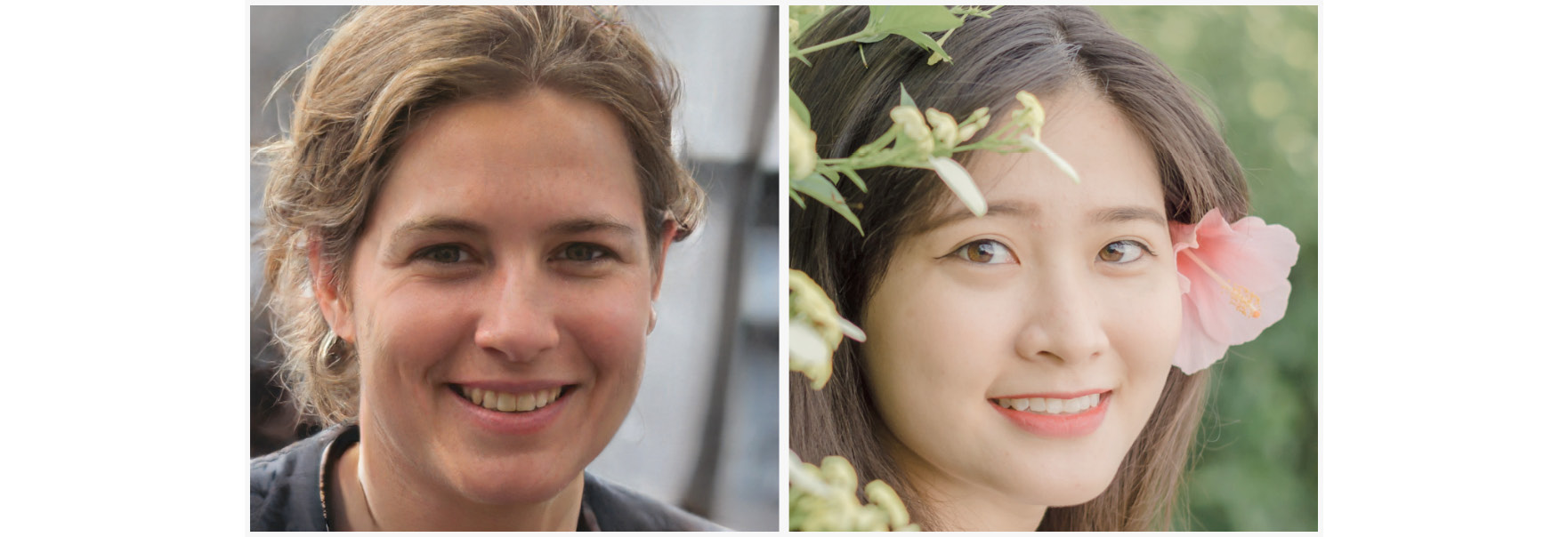
Figure 6.34: On the left is a fake image generated by a GAN, whereas the one on the right is an image of a real person

Note

Credits: http://www.whichfaceisreal.com

Coming back to the traditional methods of performing image augmentation, we perform the operations mentioned previously, such as flipping images, and then train our model on both the original and the transformed image. Let's say we have the following flipped image of a cat on the left:

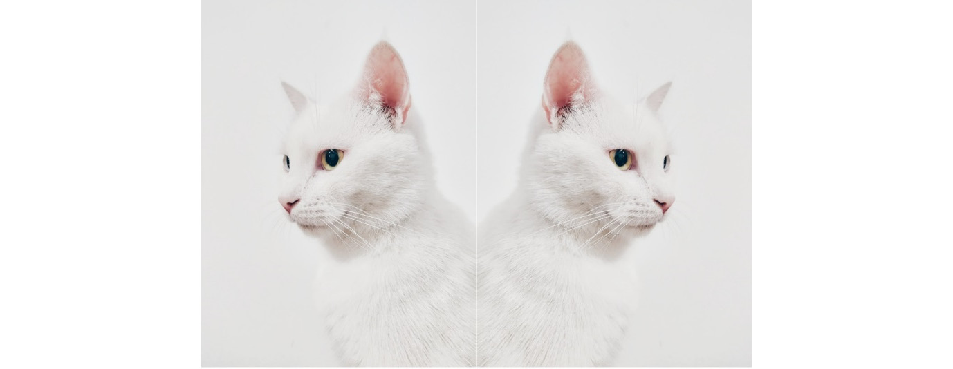
Figure 6.35: Normal picture of the cat on the right and flipped image on the left

Now, a machine learning model trained on this left image would have a hard time recognizing the flipped image on the right as that of a cat because it is facing the other way. This is because the convolutional layers are trained to detect images of cats looking to the left only. It has created rules about the position of the different features of a body.

Thus, we train our model on all the augmented images. Data augmentation is the key to getting the best results from a CNN model. We make use of the ImageDataGenerator class in Keras to perform image augmentations easily. You will learn more about generators in the next section.

Generators

In the previous chapter, we discussed how big datasets could lead to problems in training due to the limitations in RAM. This problem is a bigger issue when working with images. Keras has implemented generators that help us get batches of input images and their corresponding labels while training on the fly. These generators also help us perform data augmentation on images before using them for training. First, we will see how we can make use of the ImageDataGenerator class to generate augmented images for our model.

To implement data augmentation, we just need to change our Exercise 3 code a little bit. We will substitute model.fit() with the following:

BATCH_SIZE = 32

aug = ImageDataGenerator(rotation_range=20,

width_shift_range=0.2, height_shift_range=0.2,

shear_range=0.15, zoom_range=0.15,

horizontal_flip=True, vertical_flip=True,

fill_mode=”nearest”)

 

log = model.fit_generator(

aug.flow(x_train, y_train, batch_size= BATCH_SIZE),

validation_data=( x_test, y_test), steps_per_epoch=len(x_train) // BATCH_SIZE, epochs=10)

Let's now look at what ImageDataGenerator is actually doing:

• rotation_range: This parameter defines the maximum degrees by which the image can be rotated. This rotation is random and can be of any value less than the amount mentioned. This ensures that no two images are the same.
• width_shift_range/height_shift_range: This value defines the amount by which the image can be shifted. If the value is less than 1, then the value is assumed to be a fraction of the total width. If it is more than 1, it is taken as pixel. The range will be in the interval (-shift_range, + shift_range).
• shear_range: This is the shearing angle in degrees (counter-clockwise direction).
• zoom_range: The value here can either be [lower_range, upper_range] or be a float, in which case the range would be [1-zoom_range, 1+zoom_range]. This is the range for the random zooming.
• horizontal_flip / vertical_flip: A true value here makes the generator randomly flip the image horizontally or vertically.
• fill_mode: This helps us decide what to put in the whitespaces created by the rotation and searing process.

  constant: This fills the white space with a constant value that has to be defined using the cval parameter.

  nearest: This fills the whitespace with the nearest pixel.

  reflect: This causes a reflection effect, much like a mirror.

  wrap: This causes the image to wrap around and fill the whitespace.

The generator is applying the preceding operations randomly on all the images it encounters. This ensures that the model does not see the same image twice and mitigates overfitting. We have to use the fit_generator() function instead of the fit() function when working with generators. We pass a suitable batch size to the generator depending on the amount of free RAM we have for training.

The default Keras generator has a bit of memory overhead; to remove this, you can create your own generator. To do this, you will have to make sure you implement these four parts of the generator:

1. Read the input image (or any other data).
2. Read or generate the label.
3. Preprocess or augment the image.

   Note

   Make sure to augment the images randomly.

4. Generate output in the form that Keras expects.

An example code to help you create your own generator is given here:

def custom_image_generator(images, labels, batch_size = 128):    

    while True:

          # Randomly select images for the batch           batch_images = np.random.choice(images,

                                     size = batch_size)          batch_input = []          batch_output = []           

          # Read image, perform preprocessing and get labels

          for image in batch_images:

               # Function that reads and returns the image

              input = get_input(image)

              # Function that gets the label of the image

                output = get_output(image,labels =labels)

              # Function that pre-processes and augments the image

                input = preprocess_image(input)

              batch_input += [input]              batch_output += [output]

          

          batch_x = np.array( batch_input )          batch_y = np.array( batch_output )          

            # Return a tuple of (images,labels) to feed the network           yield(batch_x, batch_y)

Implementing get_input, get_output, and preprocess_image is left as an exercise.

Exercise 53: Classify CIFAR-10 Images with Image Augmentation

In this exercise, we will perform classification on the CIFAR-10 (Canadian Institute for Advanced Research) dataset, similar to Exercise 52. Here, we will make use of generators to augment the training data. We will rotate, shift, and flip the images randomly:

1. Load the CIFAR-10 dataset using the Keras library:

   from keras.datasets import cifar10

   (x_train, y_train), (x_test, y_test) = cifar10.load_data()

2. Convert the data to the format that Keras requires:

   x_train = x_train.reshape(-1, 32, 32, 3)

   x_test = x_test.reshape(-1, 32, 32, 3)

3. Convert the target variable to a one-hot vector so that our network does not form unnecessary connections between the different target variables:

   from sklearn.preprocessing import LabelBinarizer

   label_binarizer = LabelBinarizer()

   label_binarizer.fit(range(10))

   y_train = label_binarizer.transform(y_train)

   y_test = label_binarizer.transform(y_test)

4. Create the model. We will use the network from Exercise 3:

   from keras.models import Sequential

   model = Sequential()

   Add the convolutional layers:

   from keras.layers import Dense, Dropout, Conv2D, MaxPool2D, Flatten, BatchNormalization

   model.add(Conv2D(32, (3, 3), activation='relu', padding='same', input_shape=(32,32,3)))

   model.add(Conv2D(32, (3, 3), activation='relu'))

   Add the pooling layer:

   model.add(MaxPool2D(pool_size=(2, 2)))

   Add the batch normalization layer, along with a dropout layer:

   model.add(BatchNormalization())

   model.add(Dropout(0.10))

5. Flatten the 2D matrices into 1D vectors:

   model.add(Flatten())

6. Use dense layers as the final layers for the model:

   model.add(Dense(512, activation='relu'))

   model.add(Dropout(0.5))

   model.add(Dense(10, activation='softmax'))

7. Compile the model using the following code:

   model.compile(loss='categorical_crossentropy', optimizer='adam',

   metrics = [‘acc'])

8. Create the data generator and pass it the augmentations you want on the data:

   from keras.preprocessing.image import ImageDataGenerator

   datagen = ImageDataGenerator(

       rotation_range=45,

       width_shift_range=0.2,

       height_shift_range=0.2,

       horizontal_flip=True)

9. Train the model:

   BATCH_SIZE = 128

   model_details = model.flow(datagen.flow(x_train, y_train, batch_size = BATCH_SIZE),

                       steps_per_epoch = len(x_train) // BATCH_SIZE,

                       epochs = 10,

                       validation_data= (x_test, y_test),

                       verbose=1)

10. Check the final accuracy of the model:

    score = model.evaluate(x_test, y_test)

    print(“Accuracy: {0:.2f}%”.format(score[1]*100))

    The output is shown as follows:

Figure 6.36: Model accuracy output

Congratulations! You have made use of data augmentation to make your model recognize a wider range of images. You must have noticed that the accuracy of your model decreased. This is due to the low number of epochs we trained the model on. Models in which we use data augmentatio n need to be trained for more epochs. You will also see that you can train for a lot more epochs without worrying about overfitting. This is because every epoch, the model is seeing a new image from the dataset. Images are rarely repeated, if ever. You will definitely see an improvement if you run the model for more epochs. Experiment with more architectures and augmentations.

Here you can see an incorrectly classified image. By checking the incorrectly identified images, you can gauge the performance of the model and can figure out where it is performing poorly.

y_pred = model.predict(x_test)

incorrect_indices = np.nonzero(np.argmax(y_pred,axis=1) != np.argmax(y_test,axis=1))[0]

labels = ['airplane', 'automobile', 'bird', 'cat', 'deer', 'dog', 'frog', 'horse', 'ship', 'truck']

image = 2

plt.imshow(x_test[incorrect_indices[image]].reshape(32,32,3))

plt.show()

print("Prediction: {0}".format(labels[np.argmax(y_pred[incorrect_indices[image]])]))

See the following screenshot to check the incorrect prediction:

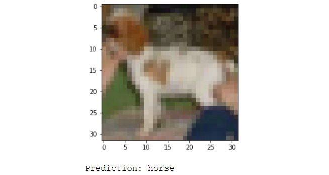
Figure 6.37: Incorrect prediction from the CNN model that was trained on augmented data

Activity 18: Identifying and Augmenting an Image

In this activity, we will attempt to predict if an image is of a cat or a dog, like in Activity 17. However, this time we will make use of generators to handle images and perform data augmentation on them to get better results:

1. Create functions to get each image and each image label. Then, create a function to preprocess the loaded images and augment them. Finally, create a data generator (as shown in the Generators section) to make use of the aforementioned functions to feed data to Keras during training.
2. Load the test dataset that will not be augmented. Use the functions from Activity 17.
3. Create a CNN that will identify if the image provided is of a cat or a dog. Make sure to make use of regularization.

   Note

   The solution for this activity can be found on page 373.

You should find that the test set accuracy for this model is around 72%, which is an improvement on the model in Activity 17. You will observe that the training accuracy is really high, at around 98%. This means that this model has started to overfit, much like the one in Activity 17. This could be due to a lack of data augmentation. Try changing the data augmentation parameters to see if there is any change in accuracy. Alternatively, you can modify the architecture of the neural network to get better results. You can plot the incorrectly predicted images to get a sense of how well the model performs.

import matplotlib.pyplot as plt

y_pred = model.predict(validation_data[0])

incorrect_indices = np.nonzero(np.argmax(y_pred,axis=1) != np.argmax(validation_data[1],axis=1))[0]

labels = ['dog', 'cat']

image = 7

plt.imshow(validation_data[0][incorrect_indices[image]].reshape(50,50), cmap=plt.get_cmap('gray'))

plt.show()

print("Prediction: {0}".format(labels[np.argmax(y_pred[incorrect_indices[image]])]))

An example is shown in the following screenshot:

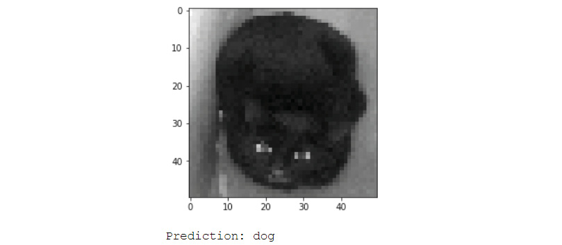
Figure 6.38: Incorrect prediction of a cat by the data augmentation CNN model

Summary

In this chapter, we learned what digital images are and how to create machine learning models with them. We then covered how to use the Keras library to train neural network models for images. We also covered what regularization is, how to use it with neural networks, what image augmentation is, and how to use it was our focus. We covered what CNNs are and how to implement them. Lastly, we discussed various image preprocessing techniques.

Now that you have completed this chapter, you will be able to handle any kind of data to create machine learning models. In the next chapter, we shall learn how to process human language.