
Chapter
8
Replication Technologies
TOPICS COVERED IN THIS CHAPTER:
- Synchronous replication
- Business continuity
- Asynchronous replication
- Array-based replication
- Database log shipping
- Logical volume manager snapshots
- Hypervisor replication and snapshots
- Multi-site replication topologies
- Array-based snapshots
- Array-based clones
 This chapter presents replication and snapshot technologies and how they fit into business continuity and disaster recovery planning and execution. You'll look at the types of remote replication technologies, such as synchronous and asynchronous, and the impact each has on network links required to support them. You'll also look at how replication and snapshot technologies are implemented at different layers in the stack, such as in the storage array, in the hypervisor, in a volume manager, and within applications and databases. Finally, you will see how to make sure applications and filesystems are consistent, and why consistency is important.
Business Continuity
Replication and snapshot technologies are a fundamental component of just about every business continuity (BC) plan. Business continuity is all about keeping the business running in the event of a disaster. Because we use the term disaster, business continuity is often referred to as disaster recovery (DR). And when we use the term disaster, we mean any event that impacts the smooth-running business IT systems. Common examples of events that are considered disasters include the following:
- System failures and crashes
- Power failures
- Water leaks
- Natural disasters
- Human errors
One example is an approaching hurricane or major storm that will affect the site that is running your live business applications. As such a storm approaches, you will want to move these applications so they are running out of another site that will not be affected by the storm.
Another example is the failure of a large shared storage array—such things do happen—requiring you to bring affected applications back up on another array, potentially in another site.
All of these things require careful planning and plenty of practice!

While it is true that things don't go wrong too often in the storage world—especially when compared with the network world—it's fair to say that when things do go wrong in the storage world, they tend to go wrong in style! Although storage issues are few and far between, when they happen they tend to be big.
It's vital to understand that in today's world, most businesses are so reliant upon technology that it would be true to say that the technology is the business. No technology = no business! Unfortunately, it can often be quite hard to convince C-level management of this fact, even though they won't hesitate to come and shout at you when systems are down and the business is losing money!
Although 99 percent of businesses don't need to worry about hurricanes, many businesses have planned events that require them to move application services to an alternative site while maintenance work takes place. These planned events might include things such as annual power maintenance or other maintenance and engineering (M&E) works.
But business continuity is more than just making sure IT systems are up and running. It's all about making sure you can still effectively run the business. For example, it's no good having all storage and servers up and running in a remote DR site if people can't access those services or if performance is so poor that the business cannot effectively operate.
This chapter concentrates on the data replication components of business continuity and discusses volume snapshots. However, other key factors in a business continuity plan include backups, workplace recovery (desks for staff to work from if HQ is down), working from home, effective communications during the disaster, bringing servers and applications back online, and so on.
At the end of the day, everyone in IT has a responsibility to the business, as well as the customers of the business, to ensure that the business can operate in the event of a disaster. If IT infrastructure goes down and you do not have a plan of how to get the business back up and running, you risk losing your job, other people's jobs, and potentially the entire business. So, no pressure!
Having a plan of how to get the business back up and running doesn't just mean scribbling a few ideas on a notepad somewhere. We're talking about proper plans and proper practice runs (sometimes called rehearsals). Rehearsals are absolutely vital in managing effective and reliable business continuity. Test your plans, learn from the things that didn't go to plan—and trust me, things never go quite according to plan—and then test again and again! You absolutely do not want to be testing your BC plans for the first time in the heat of a severity 1 disaster!
It's also important to understand the business importance of your applications. Mature organizations have all their applications mapped against priorities or tiers. These priorities are then used as part of the decision-making process when determining the order in which applications are recovered in the event of a disaster. For example, all priority 1 applications might be brought back online first, and you might have agreed with management that you will have all priority 1 applications back up and running within 2 hours. Priority 3 applications will be less important to the business, and you might have agreed with management that these will be back up and running within 10 hours of the disaster. Mature organizations rehearse their BC plans regularly—this cannot be stressed enough!

Do not make the mistake of thinking that systems used internally by the IT department aren't as important as priority 1, mission-critical, line-of-business applications in the event of a disaster. Your chances of being able to recover mission-critical applications will be severely reduced if you cannot log on to the systems required to recover your mission-critical applications. IT systems such as remote-access gateways that allow staff to log on remotely and management servers to run scripts and tools are important and often need to be up before you can even start recovering business applications. You can't run scripts to start business applications if you can't get logged on in the first place!
Some infrastructure-type applications that often get overlooked include email and corporate chat tools, which can be vital in coordinating efforts in the event of a disaster. During a disaster, communication is often the number one priority. There is no point in everyone in IT busily working on recovering from the disaster if everyone is working in different directions.
OK, that covers the background and the important basics. Before you start looking in more detail at the technologies underpinning it all, let's take a quick look at some of the language related to business continuity:
Recovery Point Objective (RPO) This is the point in time to which a service is restored/recovered. In other words, if you have an RPO of 15 minutes, you need to be able to recover an application or service to the state it was in no more than 15 minutes before the disaster occurred. To do that, you could arrange for backups to be taken every 15 minutes. For example, a backup of a database taken at 8:30 a.m. can recover the state of the database to what it was at the time of the backup (8:30 a.m.). However, if a disaster strikes at 8:44 a.m., the backup cannot recover the database to how it was between 8:30 and 8:44. The backup can recover the application only to the state it was in at exactly 8:30—the exact time the backup was taken. As a note, backups are vital, but do not normally provide the best RPOs. For a more granular RPO, frequent snapshots of continuous data protection (CDP) products are often a better choice.
Recovery Time Objective (RTO) This refers to how long it takes to get an application or service back up and running. If we go with the same disaster at 8:44, and it takes you 2 hours to recover the database to the state it was in 15 minutes prior to the disaster, then your RTO should be no less than 2 hours. In terms of RTO, this is a period of time you and the business manager pre-agree that it will take to recover an application or service. So if you know that at best it will take you 2 hours to recover a service, you should agree to a more realistic RTO of something like 3 hours. Of course, if you encounter a severe unexpected disaster and you have to recover 20 applications, each with an RTO of 2 hours, you will probably not be able to recover them all within the 2 hours.
Service-Level Agreement (SLA) An SLA is a level of service that you agree to maintain with a customer or business unit, and you will see SLAs everywhere. You might have an SLA on a high-performance storage array that it will provide an I/O response time of less than 30 ms. In the arena of business continuity, SLAs tend to incorporate RPO and RTO. An important point to note about SLAs and RTOs is that although you might be able to recover email, finance systems, trading, or reporting systems within 2 hours, you will probably not be able to recover all of them in 2 hours if they are all affected by the same disaster. Put another way, you can recover email or finance systems or trading systems within 2 hours, but you cannot recover email and finance and trading within the same 2 hours! Such things are vital for business management to understand well in advance of any disasters.
Services When talking about BC, it is important to talk in terms of services or applications, meaning a collection of servers and other technology resources. For example, the business will not care if you can recover all your front-end web servers if you haven't recovered any of the required backend database servers that the web servers need to talk to. Protection and recovery should be thought of and performed in terms of services supplied to the business.
Invoking DR Invoking DR usually means bringing an application or service up at a remote site. For example, flaky hardware on a database server that causes the database server to be up and down would probably cause you to invoke DR for that application/service by moving all required components over to standby systems in your DR site. It is possible to invoke DR for a single server, an entire application, an entire service, or even an entire estate. Invoking DR for an entire estate is usually no mean feat!
Reduced Resiliency Reduced resiliency, in BC terms, usually refers to a loss of the ability to invoke DR or a loss of high availability. An example of losing the ability to invoke DR is losing power at your DR site, meaning you cannot recover services to that site if you experience issues at your main production site. An example of loss of high availability is losing one SAN fabric; under normal operating circumstances, you will probably run dual redundant fabrics, and losing one of those fabrics will reduce your resiliency. The thing to note about reduced resiliency is that your business applications are not usually impacted; you are just running at higher risk that a failure could incur more downtime than you can tolerate.
High Availability (HA) HA refers to IT designing and deploying solutions in a resilient manner. A common example in the storage world is deploying dual independent fabrics, with each server connected to both fabrics, so that if one fabric fails, service can continue over the surviving fabric. Only if both fabrics fail simultaneously will DR have to be invoked. A major goal of HA is to prevent having to invoke DR unless absolutely necessary. This is because HA usually doesn't require any service outage. In the dual fabric example, when one fabric fails, the other immediately takes over without any service outage. This is usually not the case when invoking DR. Invoking DR nearly always involves a short amount of service downtime.
When it comes to business continuity, there is a lot to consider and a lot to be missed if you don't test your business continuity plans regularly. Test them regularly!
Replication
Replication is a core component to any BC and DR strategy. However, it is only one component. Replication must be combined with effective backups of data and a whole lot more in order to form a viable business continuity strategy.
In this chapter, the term replication refers specifically to remote replication—copying data from a primary site to a remote secondary site. Sometimes this remote replication technology is referred to as mirroring, whereby you create a remote mirror.
You use remote replication to keep copies of your data at one or more remote sites. Two major uses for these remote replicas are as follows:
- Business continuity
- Reporting and testing/development
In the case of BC, remote replicas of data can often be used to recover applications and services in the event of outages such as crashed systems, failed power, water leaks, and natural disasters. In the case of reporting and testing/development use cases, remote replicas are often used as read-only copies of data that you run reports against. An advantage of using the remote replicas to run reports against is that any workload imposed on the remote replica, such as heavy read workload as a result of the report, is isolated to the remote replica and has no performance impact on the live production copy of the data.
Replication can be performed at various layers in the stack. These are the most common layers where it happens:
- Application/database layer
- Host layer (logical volume manager based in the Linux world)
- Storage layer (array based)
You'll take a look at each of these, but first let's look at a couple of important concepts that relate to replication in general, no matter where in the stack it is implemented.

Although replication technologies are great at recovering from natural disasters, they're usually no good at protecting your data from logical corruption. Logical corruptions such as viruses will be faithfully replicated. Replication also won't help you if data is accidentally deleted. Again, deletions will be faithfully replicated to your remote replicas, ensuring that data is wiped from your remote site, too.
Synchronous Replication
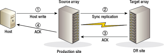
Synchronous replication technologies guarantee the remote replica to be up-to-date with the source copy of the data, which we sometimes call zero data loss. But to achieve this, synchronous replication technologies have a negative impact on performance. The reason for this is that all writes to a volume that is synchronously replicated are committed to both the source and the remote replica before the write is considered complete. This ensures that the source and target are always in sync, but it also means that the write data must travel all the way to the remote replica, and then an acknowledgment must return from the remote replica, before the write is considered complete. This round-trip to the remote replica and back can take a fairly significant amount of time (several milliseconds) and is dependent on the distance between the source and the target.
Synchronous replication offers zero data loss, which gives an RPO of zero. However, the consistency of the replica might require you to perform additional work to bring it into a consistent state. This extra work might have an impact on the RTO that you agree upon with the business management.
Figure 8.1 shows a storyboard of array-based synchronous remote replication.
Replication Distances and Latency
Replication latency is impacted by several factors, including the technology and equipment involved, the number of routers that have to be traversed en route, and the distance between the source and target. A good rule of thumb when it comes to latency and distance is to assume about 1 ms of latency for every 100 miles between the source and target. Of course, if you have to traverse a lot of routers as part of that journey, your latency will increase as each router has to process your packets.
Network latency can be (somewhat crudely) tested by using the ping command. The following ping command shows the round-trip time from a machine in London to a machine in New York over a corporate Multiprotocol Label Switching (MPLS) network. The distance between London and New York is roughly 3,500 miles, and the average round-trip time (RTT) is 77 ms—about 38.5 ms there, and another 38.5 ms back. Assuming a latency of 1 ms for every 100 miles, this gives us a distance between the London-based system and New York–based system of 3,850 miles. The math is 77 ms / 2 = 38.5 ms (because the ping command is telling us the time it takes for a packet to get from London to New York and then back again). Then we take 38.5 ms and multiply by 100 to convert the milliseconds into miles, and we get 3,850 miles.
The names and IP addresses shown in the following output have been modified so they do not represent real names and IP addresses:
C:users
igelpoulton>ping nydc01

Pinging nydc01.company-internal-network.com [10.11.12.13] with 32 bytes of data:
Reply from 10.11.12.13: bytes=32 time=77ms TTL=52
Reply from 10.11.12.13: bytes=32 time=76ms TTL=52
Reply from 10.11.12.13: bytes=32 time=77ms TTL=52
Reply from 10.11.12.13: bytes=32 time=77ms TTL=52

Ping statistics for 10.11.12.13:
    Packets: Sent = 4, Received = 4, Lost = 0 (0% loss),
Approximate round trip times in milli-seconds:
    Minimum = 76ms, Maximum = 77ms, Average = 77ms
Generally speaking, 100 miles is the upper limit on distances covered by synchronous replication technologies. Less than 100 miles is preferred. Either way, the key groups to engage when making decisions like this are as follows:
- Storage vendor
- Application vendor
- Network team
Your storage vendor and application vendors will have best practices for configuring and using replication, and you will definitely want to abide by their best practices. Your network should be able to provide accurate data about the network that your replication traffic will be transported over. Don't try to do it all on your own and hope for the best. Do your research and talk to the right people!
Replication Link Considerations
When it comes to replication, the transport network for your replication traffic is vital. A flaky network link, one that is constantly up and down, will have a major impact on your replication solution.
Synchronous replication solutions tend to be the worst affected by flaky network links. For example, in extreme cases, an unreliable network link can prevent updates to an application from occurring. This can be the case if the volumes that are being replicated are configured to prevent writes if the replication link is down; you may have certain applications and use cases where it is not acceptable for the source and target volumes to be out of sync. In the real world, 99.9 percent of businesses choose not to stop writes while the network is down. However, if you don't stop writes to the source volume when the replication link is down, the target volume will quickly become out of sync. And if you have an SLA against those volumes that states they will have an RPO of zero—meaning you can recover the application or service to the exact time of the outage—then you will be in breach of your SLA.
But problems with synchronous replication can be caused by factors other than links being down. A slow link, or one that's dropping a lot of packets, can slow the write response to source volumes because new writes to the volume have to be replicated to the remote system before being acknowledged back to the host/application as complete. Any delay in the replication process then has a direct impact on the performance of the system.
Synchronous replication configurations always require robust and reliable network links. But if you happen to have applications and use cases requiring you to fence (stop writing to) volumes when the replication link is down, it is even more important that the network circuits that support your replication links are robust. In these situations, multiple network links in a highly available configuration may be required.
Because the replication network is so important in the context of synchronous replication, it is quite common to deploy multiple diverse replication networks between your source and target sites. Depending on the technologies in use, these diverse replication networks—diverse routes often via diverse telecom providers—can work in either an active/active or active/standby configuration. The design principle is that if one replication network fails, the other can handle the replication traffic with minimum disruption.
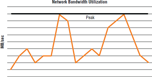
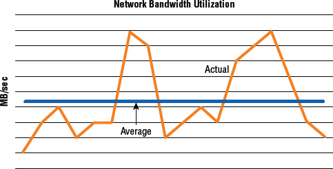
The sizing of your replication network—sometimes called network link—is also of paramount importance in synchronous replication configurations. If you get the sizing wrong, you will either be paying way over the odds or find yourself in the uncomfortable position of not being able to meet your RPO SLAs. An important design principle for synchronous replication configuration is sizing network bandwidth for peak traffic, including bursts. For example, if during high bursts of traffic the replication network is saturated and delay is introduced to the replication process, additional latency will be added to each write transaction while the source volume waits for the write transaction to be confirmed as complete at the target array, at the other end of the replication link.
Figure 8.2 shows network bandwidth utilization. If this link is to support a synchronous replication configuration, it will need to be sized to cope with the peak bursts of traffic.
Another important point to note, especially on shared IP networks, is that replication traffic can consume bandwidth and reduce performance of other applications using the shared network. Make sure you work with the network guys to put policing or other forms of network bandwidth throttling in place.
Asynchronous Replication
In many design respects, asynchronous replication is the opposite of synchronous. While synchronous replication offers zero data loss (RPO of zero) but adds latency to write transactions, asynchronous replication adds zero latency to write transactions, but will almost always lose data if you ever need to recover services from your remote replicas.
The reason that asynchronous replication adds no overhead to write transactions is that all write transactions are signaled as complete as soon as they are committed to the source volume. There is no required wait until the transaction is sent across the replication network to the target systems and then signaled back as complete. This process of copying the transaction over the replication network to the target is performed asynchronously, after the transaction is committed to the source. Of course, although this removes the performance penalty of synchronous remote replication, it introduces the potential for data loss. This potential for data loss occurs because the target volume will almost always be lagging behind the source volume. Exactly how far behind depends on the technology involved. It is not uncommon with some technologies for the target volume to be as far as 15 minutes or more behind the source—meaning that you could lose up to 15 minutes’ worth of data if you lose your source volumes and have to recover services from the target volumes.
Another advantage of asynchronous replication technologies is that they allow the distances between your source and target volumes (or arrays) to be far larger than with synchronous replication technologies. This is because the RTT between the source and target is less important. After all, write performance is no longer affected by the latency of the replication network. In theory, distance between source and target volumes can be almost limitless. However, in practice, many technologies struggle over distances of more than 3,000 miles. This means you may struggle to replicate your data from an office in Sydney, Australia, back to a data center in New York (a distance of approximately 10,000 miles). In scenarios like this, it's more common to have a data center in the Asia-Pacific region that acts as a regional hub that all offices in the Asia-Pacific region replicate to.
There is also no requirement to spec network connections for asynchronous replication configurations to cope with peak demand. Therefore, network links for asynchronous replication can be cheaper, which can be a great cost saving.
Of course, all of this is of use only if your services, applications, and users can cope with the potential of losing data in the event of a disaster.
The term invoke DR (disaster recovery) refers to bringing an application up by using its replicated storage. The process normally involves failing the entire application over to a remote standby system. The process is usually disruptive, involves a lot of people, and can take up to several hours if there are a lot of applications and services that need failing over to DR.
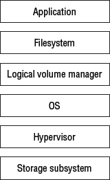
That is enough about synchronous and asynchronous replication for now. Let's take a look at how replication is performed at the different layers in the stack, starting with the application layer. Figure 8.3 shows some components of the storage technology stack with the application layer sitting on the top. As we talk about how replication is performed at different layers in the stack, we'll start out at the top with the application layer, and work our way down the stack to the lower layers.
Application-Layer Replication
Applications sit on top of the storage stack. They are the highest level in the stack, above logical volume managers, hypervisors, and storage arrays.
Application-layer replication performs all the hard work of replication, at the application server. There is no offloading of replication tasks and replication management to the storage array. This hard work consumes CPU and memory resources of the application server, and although this was once seen as a big no-no, the recent advancements in CPU technology and the massive amounts of memory common in most of today's servers means that this hard work of replication can often be easily handled by the application server.
The major advantage of application-layer replication is undoubtedly application awareness, or application intelligence. The term application-aware replication means that the replication technology is tightly integrated with the application, often as a component of the application itself. And this tight integration of the replication engine and the application produces replicas that are in an application-consistent state, meaning that the replicas are perfect for quickly and effectively recovering the application. These kinds of application-consistent replicas are in stark contrast to application-unaware replicas—those that are not performed at the application layer or that are without any integration with the application—which are often in an inconsistent state and can require additional work in order for the application to be successfully recovered from them.
Popular examples of application-layer replication include technologies such as Oracle Data Guard and the native replication technologies that come with Microsoft applications such as Microsoft SQL Server and Microsoft Exchange Server.
Let's look at a couple of popular application-based replication technologies:
- Oracle Data Guard
- Microsoft Exchange Server
By the way, both of these replicate over IP.
Oracle Data Guard
Oracle databases can be replicated via storage array–based replication technologies or Oracle Data Guard, Oracle's own application-layer remote-protection suite. Both types of replication are extensively used in the real world, but there has recently been a shift toward using Data Guard more than array-based replication. Let's take a quick look at Data Guard.
Oracle Data Guard, sometimes shortened to DG, is an application-based remote replication technology. Because it is written by Oracle specifically for Oracle, it has a lot of application awareness that array-based replication doesn't have. The net result is that Data Guard replicas are transactionally consistent.
In a DG configuration, a production database is known as the primary, and each remote disaster recovery copy of the database is known as a standby. There can be multiple standby copies of a primary database, but only one primary database in a DG configuration. Standby databases can, and should, be located in geographically remote locations so that if the site that hosts the primary database fails, standby databases are not affected and can be transitioned to primary.
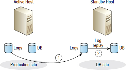
DG is a form of log-shipping technology; redo logs from the primary are shipped to the standby databases, where they are applied to ensure transactionally consistent standby databases. Figure 8.4 shows a simple log-shipping configuration.
Application-layer replication can also be more bandwidth efficient than replication performed at lower layers in the stack, such as the array. For example, when replicating databases, array-based replication technologies have to replicate all changes to both the database and log file volumes. By comparison, application-layer replication based on log-shipping technology replicates changes to only the log files. Application-layer replication can also be more bandwidth efficient than array-based replication that is based on snapshot technologies. Snapshot-based replication technologies tend to replicate in units of extents, which can be far larger than the changed data they are required to replicate. For example, a 4 KB change to a 1 MB extent will require the entire 1 MB extent to be replicated.
Data Guard supports two types of standby databases:
Physical A physical standby database is ensured to be an exact physical copy of the primary database. This includes an identical on-disk block layout and an identical database configuration including row-for-row exactness, meaning that the standby will have the same ROWIDs and other information as the primary. This type of standby works by shipping the redo logs from the primary database and applying them directly to the standby database as redo transactions. Physical standby databases can be mounted as read-only while in a DG configuration.
Logical A logical standby database contains exactly the same data as the primary database, but the on-disk structures and database layout will be different. This is because the redo logs are converted into SQL statements that are then executed against the standby database. This difference allows the logical standby database to be more flexible than the physical standby database, resulting in it being able to be used for more than just DR and read-only (R/O) access.
Both standby database types are guaranteed to be transactionally consistent. And both perform data integrity checks at the standby DB before the replicated data is committed.
Oracle Data Guard also allows for both switchover and failover. Switchover is the process of manually transitioning a standby database from the standby role to the primary role. Usually associated with planned maintenance tasks, switchover guarantees zero data loss. Failover is usually an automatic process that occurs when the primary database fails. Failover can also be configured to guarantee zero data loss.
Microsoft Exchange Server Replication
Microsoft Exchange Server is another popular application that has its own native replication engine. You can do array-based replication, or you can do Exchange native replication. The choice is yours. Recently, there has been a real push toward using Exchange native replication rather than array-based replication. Both work, but Exchange's own native application-layer replication tends to be cheaper and has more application awareness. You also don't need to involve the storage team when failing over. On the downside, though, it doesn't support synchronous replication.
Like Oracle Data Guard and many other application-layer replication technologies that are database related, Exchange replication is based on an active/passive architecture that allows you to have more than one standby copy of a database. It also utilizes log shipping; you ship the transaction logs to a remote Exchange server where they are applied. Like most application-based replication technologies, it supports both switchover and failover.
As of Exchange 2010, the fundamental unit of replication is the data availability group, or DAG for short. A DAG is a collection of Exchange Servers that host active and standby copies of mailbox databases, as shown in Figure 8.5.
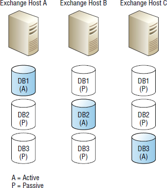
In Figure 8.5, any server in the DAG can host a copy of a mailbox database from any other server in the DAG. Each server in the DAG must have its own copy of any mailbox database that it is configured to be active or standby for. Having a single copy of a database on shared storage that is seen and shared by multiple mailbox servers is not allowed!
Within the DAG, recovery is performed at the database level and can be configured to be automatic. Because recovery is performed at the database level, individual mailbox data-bases can be failed over or switched over, and you do not have to fail over or switch over at the server level (which would affect all databases on that server).
Also, Exchange replication uses Microsoft failover clustering behind the scenes, though this is not obvious from regular day-to-day operations.
With the introduction of DAGs in Microsoft Exchange Server 2010, replication no longer operates over SMB on TCP port 445. This can make life unbelievably simpler for people who work for organizations that are paranoid about security. And what organizations aren't paranoid about security these days?
Exchange Server 2010 and 2013 both provide a Synchronous Replication API that third-party storage vendors can tap into so they can provide synchronous replication capabilities to Exchange 2010 and 2013 DAGs. They effectively replace the native log-shipping replication engine with their own array-based synchronous block–based replication.
There are plenty of other database- and application-based replication technologies, but the two mentioned here—Oracle Data Guard and Microsoft Exchange Server—provide good examples of how they work. Some of the key factors in their favor include the following:
- Cost
- Application consistency
- Simplicity
Logical Volume Manager–Based Replication
Volume managers exist further down the technology stack than applications, but higher in the stack than hypervisors and storage arrays.
Host-based volume managers, such as Linux LVM, are capable of remote replication by using long-distance LVM mirrors. On the Linux LVM front, most people still consider this both a poor-man's replication technology and somewhat risky for production environments. That is fine for labs and maybe development environments, but it is not a technology to bet the business on. That said, it can be useful, and in the case of Linux LVM, it's free.
Because LVM is agnostic about the underlying storage technology, many companies have utilized LVM mirroring to perform storage migrations, whereby the storage presented to a server is being changed from one vendor to another, and the host stays the same. Some of these migrations have been performed when the server is running but applications and databases are shut down. However, at times LVM mirroring has been successfully used to migrate lightly used databases to new storage arrays. The latter should be done with extreme care, as there is no guarantee it will work.
In the Windows world, third-party products that are implemented as filter drivers above the volume management layer are often used to provide server-based replication. A common example, and one that has been around for some time now, is Double-Take.
Hypervisor-Based Replication
Hypervisors exist further down the technology stack than applications and logical volume managers, but higher in the stack than storage arrays.
As hypervisor technologies mature, they are starting to offer more and more advanced features natively. One of these features is replication. Although sometimes seen as a poor-man's replication choice, hypervisor-based replication technologies are maturing at a fast pace and have some potential advantages over array-based replication technologies—not to mention lower costs.
So far, interest in hypervisor-based replication technologies is strongest in small and medium businesses (SMB), but it is definitely worth a look even if you consider your company to be more than SMB. VMware vSphere Replication is currently the most advanced hypervisor replication technology, so let's take a look at it as an example.
vSphere Replication
VMware vSphere now offers a native hypervisor-level replication engine that can be leveraged by Site Recovery Manager (SRM). It goes by the name of vSphere Replication.
A couple of good things about vSphere Replication include reduced costs and a simplified configuration. Both of these factors are important in 99 percent of IT environments. Costs can be reduced by not having to purchase expensive array-based replication licenses, effectively bringing the advanced features of SRM replication to more people. vSphere Replication also brings a heap of flexibility to the storage layer by allowing storage platform independence and reducing any potential vendor lock-in at the storage layer. Basically, you can use any storage underneath, and your choice of storage technology does not have to be the same at the source and target.
Be careful about using any storage and not making the effort of matching storage at the source and target. Although it reduces costs and allows more-flexible replication configurations, not matching the source and target storage has the potential to increase some of the risks surrounding the configuration. These risks include availability and performance, including potentially poor performance if you ever have to run your business on lower-performance storage in the event of a disaster.
vSphere Replication is an IP-based replication technology that works at the virtual machine disk (VMDK) level. Working at the VMDK level allows you to configure replication at a very granular level—more granular than even at the virtual machine level. For example, imagine you have a VM with four virtual disks as follows:
VMDK 1: OS partition
VMDK 2: Page-file partition
VMDK 4: Scratch partition
Now imagine you have a skinny network pipe between your data centers and want to make sure you replicate only the data that you will need in the event of a disaster. You can select to replicate only VMDK 1 and VMDK 3, and not to replicate the page file and scratch VMDK files. This could significantly ease the load placed on the replication network between sites.
On the efficiency front, vSphere Replication is intelligent enough to only replicate changed blocks for each VMDK, using a similar technology to the changed block tracking (CBT) engine used for incremental backups.
vSphere Replication also exists above the storage layer in the ESX stack, meaning that you are free to use any storage you want as the underlying storage—so long as it exists on VMware's hardware compatibility list (HCL). This is the opposite of when using array-based replication technologies that usually come with strict rules about which underlying storage platforms can replicate with each other. (Quite often these restrict you to the same vendor and same model for both the source and target.) For example, in a vSphere Replication configuration, your primary copy of a VM could be running on an iSCSI LUN from a Dell EqualLogic iSCSI storage array, but your remote offline VM might sit on a datastore on a local disk!
vSphere Replication replicates powered-on VMs (there is not much to replicate if the primary VM is powered off) from one ESXi host to another. These ESXi hosts can be in the same cluster in the same site or in different clusters at remote sites. Also, the ESXi host-based agent is installed by default, meaning no VM-based agents are required in order to use vSphere Replication.
vSphere Replication is also application aware on the Microsoft front, making API calls to the Microsoft Volume Shadow Copy Service (VSS) for the likes of Microsoft Exchange Server and Microsoft SQL Server, ensuring remote replicas are consistent and can safely and easily be recovered from.
As you can see in Exercise 8.1, standard vCenter tools are used to configure vSphere Replication as well as VM recovery. RPOs can also be configured for anywhere between a minimum of 15 minutes to a maximum of 24 hours.
EXERCISE 8.1
Configuring vSphere Replication
This exercise highlights the steps required to configure vSphere Replication (VR) via the vSphere Web Client. As a prerequisite, this example assumes that you have downloaded and are running the vSphere Replication Manager (VRM) virtual appliance and have vSphere Replication traffic enabled on a VMkernel NIC.
1. Within the vCenter Web Client, locate the powered-on VM that you want to replicate. Right-click the VM and choose All vSphere Replication Actions ![]() Configure Replication.
Configure Replication.
It is possible to configure vSphere Replication with just a single site configured in vCenter. Obviously, this kind of replication won't protect you from site failures, but it is good for practicing in your lab or for protecting against loss of datastores.
2. Choose the site you want to replicate to and click Next.
3. Choose a target datastore to replicate to (if you have only a single site, make sure the target datastore is a different datastore than the one your VM is currently in). Click Next.
4. Use the slider bar to choose an RPO between 15 minutes and 24 hours. Smaller is usually better.
5. If supported by your Guest OS, you can also choose to quiesce the VM.
6. Click Next.
7. Review your choices and click Finish.
vSphere will now make the required changes–such as injecting a vSCSI driver into the guest to manage changed block tracking–and then perform an Initial Full Sync. After the Initial Full Sync is complete, only changed blocks will be replicated.
In its current incarnation, the smallest RPO you can configure with vSphere Replication is 15 minutes. This will be fine for most use cases, but not all.
Despite its many attractive features, vSphere Replication is host based and therefore consumes host-based CPU and memory. Not always the end of the world, but in a world that demands efficient resource utilization on a platform that boasts massive server consolidation, it may not be the most efficient solution. This is especially true if you already have investment in storage array technologies.
Integrating SRM with Storage Array–Based Replication
VMware Site Recovery Manager (SRM) can be, and frequently is, integrated with array-based replication technologies, yielding an enterprise-class business continuity solution. This kind of configuration allows for replication and site recovery via common VMware tools but with the power of rock-solid, array-based replication engines that offload all the replication overhead from the hypervisor.
Only supported storage arrays work with VMware SRM via a vCenter Storage Replication Adapter (SRA) plug-in that allows vCenter and the storage array to understand and communicate with each other.
Array-Based Replication
When it comes to replication technologies, array-based replication technologies sit at the bottom of the stack, below hypervisors, logical volume managers, and applications.
In array-based replication technologies, the storage array does all the hard work of replication, freeing up host resources to serve the application. However, vanilla array-based replication technologies—those that don't have special software to make them application aware—do not understand applications. So we consider array-based replication to be unintelligent, or more important, the replica volumes it creates will usually be crash consistent at best. This means that the state of the application data in the remote replica volume will not be ideal for the application to recover from, and additional work may be required in order to recover the application from the replica data. This is one of the major reasons that array-based replication is losing popularity and is often being replaced by application-based replication technologies.
It is possible to integrate array-based replication technologies with applications. An example is the synchronous replication API that Microsoft made available with Exchange Server 2010 and 2013 that allowed storage array vendors to integrate their replication technologies with Exchange Server, effectively replacing the native Exchange Server log-shipping application-layer replication engine with the synchronous block-based replication engine in the storage array. That provided the best of both worlds: application awareness as well as offloading of the replication overhead to the storage array.
That said, array-based replication is still solid and extremely popular, and it can be integrated with applications and hypervisors via APIs.
Storage arrays tend to implement asynchronous replication in one of two ways:
- Snapshot based
- Journal based
Let's take a look at both.
Asynchronous Snapshot-Based Replication
Many storage arrays implement asynchronous replication on top of snapshot technology. In this kind of setup, the source array takes periodic snapshots of a source volume—according to a schedule that you configure—and then sends the data in the snapshot across the replication network to the target array, where it's then applied to the replica volume. Obviously, in order to do this, an initial copy of the source volume needs to be replicated to the target system, and from that point on, snapshots of the source volume are then shipped to the target system.
Because you configure the schedule, you have the ability to match it to your SLAs and RPOs. So, for example, if you have agreed to an RPO of 10 minutes for a particular volume, you could configure the replication schedule for that volume to take a snapshot every 5 minutes and replicate the snapshot data to the target volume also every 5 minutes. This would give plenty of time for the snapshot data to be transmitted over the replication network and applied to the replica volume and keep you comfortably within the RPO of 10 minutes for that particular SLA.
It's important to note that configuring a replication interval of 10 minutes for a volume that you have agreed a 10-minute RPO for, will not be good enough to achieve the 10-minute RPO. After all, the data contained within the snapshot has to be sent across the replication network and then applied at the remote site, all of which takes additional time. Because of this, some storage arrays allow you to specify an RPO for a volume, and the array then goes away and configures an appropriate replication interval so that the RPO can safely be achieved. This approach also opens up the potential for the array to prioritize the replication of volumes that are approaching their RPO threshold over those that are not.
If your array's asynchronous replication engine is based on snapshot technology, it's also important to understand whether the snapshots used for replication will count against the maximum number of snapshots supported on the system. For example, if your array supports a maximum of 256 snapshots, and you have 32 replicated volumes, each of which maintains two concurrent snapshots as part of the replication setup, those 64 replication-based snapshots could count against your system's 256 snapshots. Be careful to check this out when configuring a solution based on snapshot-driven replication. This is covered further in the discussion of array-based snapshots toward the end of the chapter.
When working with asynchronous replication solutions that are built on top of snapshot technology, make sure that you understand the underlying snapshot extent size, as it can have a significant impact on network bandwidth utilization. For example, a large extent size, say 1 MB, will have to replicate 1 MB of data over the replication network every time a single byte within that extent is updated. On the other hand, a smaller extent size, such as 64 KB, will have to replicate only 64 KB over the replication network each time a single byte in an extent is updated. So smaller is better when it comes to replication snapshot extent sizes.
A good thing about snapshot-based replication is that as long as your array has decent snapshot technology, it will coalesce writes, meaning that if your app has updated the same block of data a thousand times since the last replication interval, only the most recent contents of that data block will be shipped over the replication network with the next set of deltas (a term used to refer to changed blocks), rather than all one thousand updates.
Asynchronous Journal-Based Replication
The other popular method for implementing array-based asynchronous replication is via journal volumes. Journal-based asynchronous replication technologies buffer new writes to either cache or dedicated volumes known as either journal volumes or write intent logs before asynchronously shipping them across the replication network to the target array. Let's take a closer look at how it usually works under the hood.
In a journal-based asynchronous replication configuration, as new write data arrives at the array, it follows the normal procedure of being protected to mirrored cache and then being signaled back to the host/app as complete. However, as part of this process, the write I/O is tagged as being part of a replicated volume to ensure that it gets copied to the journal volumes as well as being copied over the replication network to the remote target array when the next replication interval arrives. The gap between the replication intervals depends entirely on your array-replication technology and how you've configured it. However, it's usually every few seconds, meaning that the kinds of RPOs offered by journal-based asynchronous replication solutions are usually lower than those offered by snapshot-based replication configurations—which tend to offer minimum RPOs of 5 minutes.
Journal-based asynchronous replication can apply write sequencing metadata so that when the contents of the journal volume are copied to the remote system, writes are committed to the target volume in the same order that they were committed to the source volume. This helps maintain consistency of the remote replica volumes. However, if, for whatever reason the system can no longer write updates to the journal volumes (let's say the journal volumes have filled up or failed), the system will revert to maintaining a bitmap of changed blocks. This mode of operation, known as bitmapping, allows you to keep track of changed blocks in your source volume so that only changes are sent to the remote array, but it doesn't allow you to maintain write sequencing.
Some arrays implement asynchronous replication journaling in memory, in a construct often referred to as either a memory transit buffer or sidefile. Obviously, the amount of memory available for replication journaling is limited, and during extended periods of replication network downtime, these systems usually fall back to either using journal volumes, or switching to bitmapping mode where write ordering is not maintained.
Implementations differ as to whether the source array pushes updates to the target array or whether the target array pulls the updates. For your day-to-day job, things like this should not concern you, certainly not as much as making sure you meet your SLAs and RPOs.
So that's how journal-based asynchronous replication works. Let's look at some of the important points.
It's obviously vital that these journal volumes are big enough and performant enough to cater for buffering your replication traffic. On the capacity front, this is especially important when the network link or remote array is down for any sustained period of time. As with all sizing exercises, it's a trade-off: if you size the journal volumes too big, then you're underutilizing resources and wasting money, but if you size them too small, when the replication network or the remote array is down, they can fill up and cause your replicated volumes to require a full sync when the problem is fixed. A full sync is not something you want to be performing often.
As an example, assume a 2 TB volume is being replicated. When the replication network goes down—let's say a maintenance contractor hit a cable when digging up the road outside your data center—all changes to the source volume will be buffered to the journal volumes until the replication network comes back up. If the replication link is fixed before the journal volumes fill up, all you have to replicate to the target array are the changes contained in the journal volumes. However, if the journal volumes filled up during the network link outage, your replicated volumes would almost certainly be marked as failed and require you to perform a full sync—copying the entire 2 TB volume across the replication network to the remote array. This is likely to be a lot more than just the changes contained in the journal volumes. Even over 8 Gbps of bandwidth between two sites that are less than 100 miles apart, copying terabytes of data can take hours.
Asynchronous replication solutions allow you a lot more leeway when speccing replication network connections. For starters, they don't have to be sized to cater for peak bandwidth. Arguably, they don't need to be as reliable as they do for synchronous replication. However, be careful not to under-spec them. If the bandwidth is too low or they are too unreliable, you could find yourself struggling to operate consistently within your agreed-upon SLAs.
Figure 8.6 shows network bandwidth requirements for asynchronous replication. The bandwidth utilization is captured at an hourly interval, with an average line included.
Replication Topologies
The replication topologies covered here are not restricted to array-based replication. However, this section focuses on how different replication topologies are implemented by using array-based replication, because the most complex replication topologies tend to be implemented around array-based replication.
Different storage arrays support different replication topologies. Not every array supports every replication topology, though. Make sure you do your research before trying to implement a complex replication topology, as you may find yourself in an unsupported situation. These different topologies are often a mix of synchronous and asynchronous replication, with two, three, or even four arrays, located in multiple sites at various distances apart.
Let's take a look at some example replication topologies.
The replication topologies covered throughout this section are by no means exhaustive. Plenty of other configurations are possible. Most of them tend to be complicated to configure and maintain.
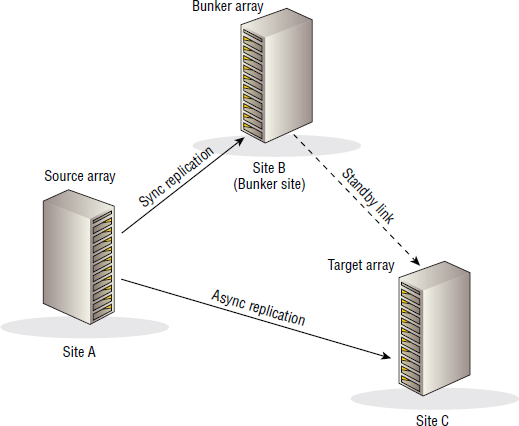
Three-Site Cascade
As the name suggests, Three-Site Cascade is based around three sites: a source site, a target site, and a bunker site between them. This configuration is shown in Figure 8.7.
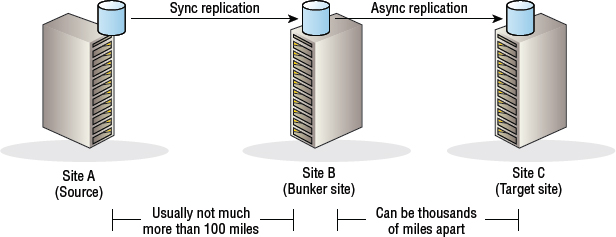
Arrays at the source and target site can't communicate with each other directly. Any data that you want to replicate from an array at the source site to an array at the target site has to first go to an array in the bunker site. A common example is a source and bunker site that are less than 100 miles apart and configured with synchronous replication. The target site is then over 100 miles away and replicated to asynchronously.
Because the target site is usually so far away from the source and bunker sites, this kind of topology lends itself well to high-performance requirements with low RPOs but the ability to survive large-scale local disasters. Take a minute to let that settle in. First of all, this solution can survive large-scale local disasters because the target site can be thousands of miles away from the source site. It can also be high performance, because the synchronous replication between volumes in the source and bunker sites can be close enough to each other that the network latency imposed on the replication traffic is low. And RPOs can be low (in fact, they can be zero), because synchronous replication offers zero data loss. Of course, if you do experience a large-scale local disaster and lose both your source and bunker sites, you'll have to recover applications at the target site that is asynchronously replicated to, so you will be lagging behind your source site and you will stand a good chance of losing some data.
Three-Site Cascade allows your applications to remain protected even if you lose the source site. This is because the bunker and target sites still have replication links between them, meaning that replication between these two sites can still occur. In simple two-site replication models, if you lose your source site and failover applications to the target site, your target site is “on its own” until you recover the source site and reconfigure replication back from the target to the original source site.
At least one major weakness of the Three-Site Cascade model is that the loss of the bunker site severs the link between the source and target site. Data at the source site cannot be replicated to the target site, and the target site starts to lag further and further behind.
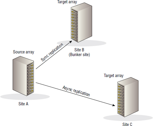
Three-Site Multi-Target
Three-Site Multi-Target has the source array simultaneously replicate to two target arrays. This topology is potentially more resilient than Three-Site Cascade, as the bunker site is no longer a soft spot in the solution. The source array has visibility of both of the other arrays in the configuration and is configured to replicate to them both, without having to rely on arrays in the bunker site. However, the major downside to Three-Site Multi-Target is that there usually isn't a connection between the two target arrays. If the source site is lost, the surviving two arrays cannot replicate to each other.
As shown in Figure 8.8, in the Three-Site Multi-Target topology, one of the remote sites is usually within synchronous replication distance, and the other a lot farther away. This kind of setup allows the topology to be able to provide zero data loss (via the local synchronous replication link) as well as the ability to ride out large-scale local disasters thanks to the asynchronous replication to the array that's a lot farther away.
Three-Site Triangle
As shown in Figure 8.9, the Three-Site Triangle topology is almost exactly the same as Three-Site Multi-Target. The only difference is the existence of an additional replication link between the two target arrays in site B and site C. As indicated in Figure 8.9, this additional replication link between the two target arrays is usually in standby mode, meaning that under normal operating circumstances, it's not used to send data. However, it can be used to replicate data in the event that the source site or source array is lost. This helps remove the major weakness of Three-Site Multi-Target, where if the source array is lost, although you have two surviving arrays, there is no way for them to replicate with each other, and you're left with two copies of your data but no way to configure the two surviving arrays into a disaster-resilient pair.
As long as your array's replication technology supports it, it's entirely possible that in the event of a disaster that causes you to lose your source array, your two remaining target arrays could communicate with each other, determine the differences between the copies of data they hold, and have to ship only the difference to each other, rather than requiring a full sync.
Local Snapshots
First, let's clarify the terminology. Snapshots are local copies (replicas) of data. Local means the snapshot exists on the same host or storage array as the source volume, making snapshots useless as recovery vehicles if you lose access to your source array. If you lose access to your source array, you obviously lose access to the source volumes and the snapshots.
Snapshots are what we call point-in-time (PIT) copies of system volumes. They provide an image of how a volume or system was at a particular point in time—at 5 p.m., for example. These snapshots can be used for a lot of things, such as rollback points, backup sources, scratch volumes to perform tests against, and so on. Snapshots are pretty flexible and are widely used in the real world.
Anyway, back to the terminology for a moment. Let's define exactly what we mean when we use the terms point-in-time and local.
Local refers to the created copies existing on the same system as the source volumes. If they are host-based snapshots, the snapshots exist on the same host as the source volume. If they are array-based snapshots, the snapshots exist on the same array as the source volumes.
Point-in-time snapshots are copies of a volume as it is at a certain time. For example, a PIT snapshot might be a copy of a volume exactly as that volume was at 9 a.m. This means they are not kept in sync with the source. This is the exact opposite of remote replicas, which are usually kept in sync, or semi-sync, with the source volume.
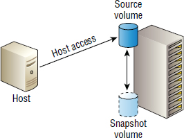
The terms source volume and primary volume refer to the live production volume, and the terms source array and primary array refer to the live production array hosting the source volume. Figure 8.10 shows a simple snapshot configuration with some terminology mapped to the diagram.
Depending on the snapshot technology you're using, you'll be able to create read-only snapshots, read-write snapshots, or both.
A vital point to note about snapshots is that they are not backups! Make sure you never forget that. Snapshots exist on the same system as the source's volume, and if you lose the source volume or source system, you also lose your snapshots. However, if you're replicating data to a remote target array, and then you take snapshots of the remote target volumes, these can work as backup copies of your source volumes because they're on a separate system, potentially in a separate site. If you lose your source system or source site, you will still have access to your remote snapshots.
Hypervisor-Based Snapshots
Most modern hypervisors now provide native snapshotting technologies. As with hypervisor-and host-based replication technologies, these snapshots consume host-based resources and do not benefit from offloading the snapshot process to the storage array. That said, they are improving and are gaining in popularity.
As VMware is a major player in the hypervisor space and has a relatively mature integrated snapshot stack, let's take a closer look at how virtual machine snapshots work in a VMware environment.
VMware Snapshots
VMware vSphere offers native virtual machine (VM) snapshotting capabilities as well as an API that third-party vendors can utilize to create and manipulate VM snapshots.
VM snapshots are PIT snapshots that preserve the state and the data in a VM at the time at which the snap was taken. For example, if you take a snapshot of a VM at 5 p.m., you have preserved an image of how that VM was at precisely 5 p.m. This snap includes the state of the VM, including whether it was powered on at the time the snap was taken, as well as the contents of the VM's memory.
When creating VM snapshots, there is an option to quiesce the VM. Quiescing a VM is all about making sure the snap you take is consistent.
For Microsoft servers—as long as VMware Tools is installed on the VM being snapped—a call is made to the VSS to quiesce the VM. VSS ensures that all filesystem buffers are flushed, and new I/O to the filesystem is held off until the snap completes. It is also possible to quiesce any VSS-aware applications such as Microsoft Exchange Server, Microsoft SQL Server, Oracle Database, Microsoft SharePoint Server, and Microsoft Active Directory. This ensures not only filesystem-consistent snapshots, but also application-consistent snapshots.
If VSS cannot be used to quiesce a system (for example, on non-Microsoft operating systems), the VMware proprietary SYNC driver manages the quiescing of the system. This can often be filesystem quiescing only. The SYNC driver effectively holds incoming writes on a system as well as flushes dirty data to disk in an attempt to make a filesystem consistent.
It is possible to have multiple snapshots of a VM. These snapshots form a tree, or chain, of snapshots. You can delete any snapshot in the tree and revert to any snapshot in the tree. However, having a large or complicated snapshot tree structure carries a performance overhead. So does having lots of snaps of a VM that experiences a high rate of change. So be careful when creating lots of snapshots. Just because you can doesn't mean you should.
Figure 8.11 shows a snapshot chain.
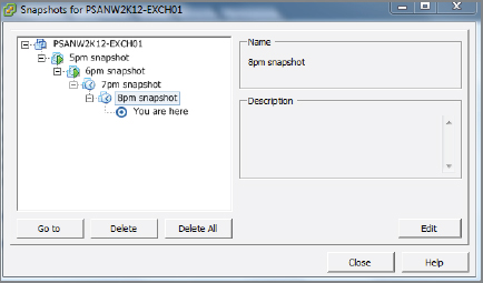
Take another look at Figure 8.11, which shows a snapshot chain in VMware Snapshot Manager. Notice the You are here at the very bottom of the snapshot chain. By default, VMware snapshots work so that you are working off the last snapshot in the chain. If you delete your snapshot, its contents will need to be merged in a process VMware calls consolidation. Assume you have a single parent (source) VM and a single snapshot. Your VM is running off the snapshot, and unless you want to lose all changes you have made to the VM since the snapshot was taken, when deleting the snapshot you need to merge the contents of the snapshot with the parent volume. This rolls up all changes since the snapshot was created back to the parent volume. If you don't consolidate the contents, you will lose all changes made since the snapshot was created.
In a VMware environment, when a snap of a VM is created, each VMDK associated with the snapped VM gets a delta-VMDK file that is effectively a redo file. There are also one or two metadata files created for storing the contents of the VM's memory, as well as snapshot management. All of these delta files are sparse files—space efficient—and work like traditional copy-on-write snapshots that start filling up with data as you make changes. Delta files obviously consume space relative to the change rate of the VM and can grow to a maximum size equal to that of the parent disk.
Snapshots are not backups! However, they are often used by VM backup applications, such as Veeam Backup & Replication. When making a backup of a VM, backup applications make a call to the VMware snapshot API to create a snap of a VM to be used as a consistent PIT copy that can be used for creating the backup. In these situations, once the backup is complete, the snapshot of the VM is released. In addition (and this is configurable and also depends on your version of vSphere) VM snapshots by default are created in the same location as the source VM that is being snapped. This usually means they have the same datastore, and therefore the same physical drives on the storage array. So a snapshot is definitely no use to you as a backup if your storage array or underlying RAID groups get toasted!
As I've mentioned backing up Microsoft servers and Microsoft applications, it is only fair to point out that the Microsoft Hyper-V hypervisor also offers fully consistent application backups for all applications that support Microsoft VSS: Exchange Server, SQL Server, Oracle Database on Windows, SharePoint Server, Active Directory, and so on.
Now let's take a quick look at how to take a VM snapshot. Exercise 8.2 shows how to do this using the vSphere Client.
EXERCISE 8.2
Taking a Manual VM Snapshot
In this exercise, you will walk through taking a manual VM snapshot by using the vSphere Client.
- From within the vSphere Client, locate the VM that you wish to take a snapshot of and right-click.
- Choose Snapshot
 Take Snapshot.
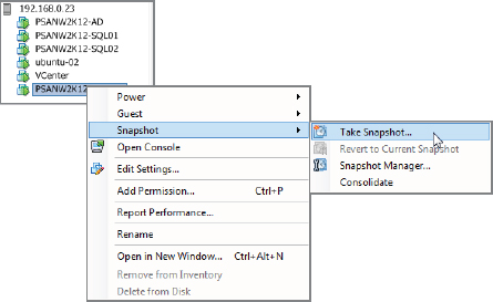
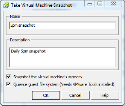
- On the screen that appears, give the snapshot a name and an optional description. Make sure to select the two check boxes, Snapshot The Virtual Machine's Memory and Quiesce Guest File System (Needs VMware Tools Installed).
- Click OK.
- The Recent Tasks view at the bottom of the vSphere Client screen shows the progress of the snapshot operation.

Array-Based Snapshots
As with array-based replication, array-based snapshots offer the benefit of offloading the snapshot work from the host system to the array. This can free up CPU and memory on the host, as well as provide faster snapshots and potentially quicker recoveries from snapshots. However, it can also add complexity to the configuration. As with all things, when possible, you should try before you buy.
As with hypervisor-based snapshots, all good array-based snapshot technologies can be made application aware by integrating with products such as Microsoft VSS to provide application-consistent snapshots. Also, when augmented with backup software, the combination of the backup software and the array-based snapshots can inform applications that they have been backed up, allowing them to truncate log files and do other tidy-up exercises often associated with backups.
In the next few pages, you will look closely at array-based snapshot technologies and concentrate on how they are implemented, as well as the pros and cons of each.
Two primary types of array-based snapshot technologies are commonly used:
- Space-efficient snapshots
- Full clones
These technologies sometimes go by various names, so I will try to be relatively consistent in this chapter. Sometimes I might call space-efficient snapshots just snapshots, and sometimes I will call full clones just clones. Also, while on the topic of vernacular, I will use the term source volume to refer to the original volume that the snapshot is taken from. I will also draw snapshots with dotted lines in the figures, to indicate that they are space efficient.
Space-Efficient Snapshots
Space-efficient snapshots are pointer based. There are two significant concepts to consider when dealing with such snapshots:
Space efficient tells us that the snapshot contains only changes made to the source volume since the snapshot was taken. These changes are sometimes referred to as deltas.
Pointer based tells us that when the snapshot is created, the entire address space of the snapshot is made up of pointers that refer I/O requests back to the source volume.
Figure 8.12 shows the concept of pointers.
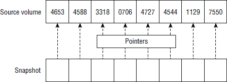
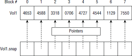
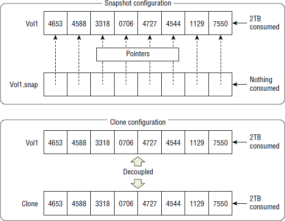
Let's look at a quick, simple example. Say that we have a source volume called Vol1. Vol1 has eight data blocks numbered 0–7. At 1 p.m. on Monday, we make a space-efficient snapshot of Vol1. At that time, all blocks in Vol1 are as shown in Figure 8.13. The snapshot of Vol1 is called Vol1.snap. When we create the snapshot, Vol1.snap consumes no space on disk. If a host mounts this snapshot and reads its contents, all read I/O will be redirected back to the original data contained in Vol1. Vol1.snap is basically an empty volume that contains only pointers (usually in memory) that redirect read I/O back to the primary volume containing the data.
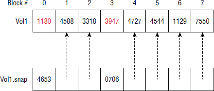
Next let's assume that by 2 p.m. Vol1 has made updates to blocks 0 and 3. Now if a host wants to read data in Vol1.snap, it will be redirected back to the source volume (Vol1) except when reading blocks 0 and 3. Because blocks 0 and 3 have changed since the time the snapshot was created, the original contents (4653 and 0706) have been copied to Vol1.snap in order to preserve an image of Vol1 as it was at 1 p.m.
At 2 p.m., the snapshot configuration looks like Figure 8.14, and the snapshot volume still represents an exact image of how the primary volume was at 1 p.m.
Snapshots are also instantly available, which means that as soon as you click the Create button, figuratively speaking, the snapshot is available to be mounted and used.
Snapshots can also be read/write, making them flexible and opening them up to lots of use cases. However, if you mount a snapshot as read/write and issue writes to it, it will obviously no longer represent the state of the source volume at the time the snap was taken. This is fine, as long as you do not plan to use the snapshot to roll back to the point in time at which the snap was taken!
If you're new to snapshot technology and this is still unclear, go grab a coffee, remove any distractions, and reread the above. It is vital that you understand how space-efficient snapshots work.
Full-Clone Snapshots
Full-clone snapshots, sometimes called just full clones or clones, are not space efficient. They don't use pointers, so they can be quite a lot simpler to understand. However, they are still PIT copies of source volumes.
At the time a clone is created, an exact block-for-block copy of the source volume is created. If the source volume is 2 TB, the clone will also be 2 TB, which will consume 4 TB of storage. You can see how full clones can quickly eat through storage.
As with snapshots, clones can be read/write, and as soon as you write to a clone (or snapshot), it no longer represents the state of the source volume at the time the clone was created. This makes it no use as a vehicle to roll back to the state the source volume was in at the time the clone was created. However, it can be useful for testing and other purposes.
How Instantaneous Cloning Works
Most array-based cloning technologies provide instantaneous clones. Just the same as with space-efficient snapshots, this means that they are immediately available after you click Create.
But how can a clone of a large multiterabyte volume be instantly available? Surely it takes a long time to copy 2 TB of data to the clone volume?
Instantaneous clones generally work as follows. When the clone is created, the array starts copying data from the source volume to the clone across the backend as fast as possible, although it is careful not to slow down user I/O on the front end. If you read or write to an area of the clone that is already copied, obviously that is fine. However, if you want to read an area of the clone that has not been copied yet, the array will either redirect the read I/O to the source volume for the blocks in question or it will immediately copy those blocks across from the source to the clone so that the read I/O does not fail. Either way, the operation is performed by the array in the background, and hosts and applications should not notice any difference.
If your clones are read/write clones, any write I/Os to an area of a clone that has not yet been copied from the source can just be written straight to the clone volume, and the respective blocks from the source volume no longer need to be copied across.
Figure 8.15 compares a space-efficient snapshot of a 2 TB volume with a full clone of a 2 TB volume at the time the snap/clone was taken.
Obviously, over time the snapshot starts to consume space. How much space depends entirely on your I/O profile. Lots of writes and updates to the source volume will trigger lots of space consumption in your snapshot volume.
So if full clones consume loads of disk space, why bother with them, and why not always go for space-efficient snapshots? There are a couple of common reasons:
- Reading and writing to a full clone has no effect on the performance of the source volume. You can hammer away at the clone without affecting the source volume's performance. This can be useful for a busy database that needs backing up while it is busy; you can take a clone and back up the clone. You could also use a clone of the same busy database as a reporting database so that reports you run against the clone don't impact the performance of the database. This works because the full clone is fully independent of the source, should be created on separate spindles, and contains no pointers. Conversely, space-efficient snapshots share a lot of data with their source volumes. If you hammer the snapshot with intensive read and write I/O, you will reference some data blocks shared with the source and therefore hammer the source volume.
- Full clones are fully independent of the source volumes. If the physical drives that the source volume is on fail, the clone will not be affected (as long as you don't keep the source and clone on the same drives). Because space-efficient snapshots rely on the source volume, if the disks behind the primary volume fail, the source and the space-efficient snapshot will fail.
In the modern IT world, where budgets are tight and ever shrinking, snapshots tend to be far more popular than full clones, so we'll spend a bit more time going into the details of array-based, space-efficient snapshots.
Snapshot Extent Size
Snapshots by their very nature are space efficient. One of their major strengths is that they take up very little space. So when it comes to space-efficient snaps, the more space we can save, the better. Smaller snapshot extent sizes are better than large snapshot extent sizes. So a snapshot extent size of 16 KB is better than one of 256 KB. Although these might seem like small numbers, on large systems that have hundreds of snapshots, the numbers can quickly add up.
The same goes for asynchronous replication technologies that rely on an array's underlying snapshot technology. In these situations, arrays with larger snapshot extent sizes will have to replicate larger amounts of data to the remote system.
Reserving Snapshot Space
Some storage arrays, especially older arrays, require you to set aside capacity to be used as snapshot reserve space. This space is then used to store data associated with snapshots. If you expect your source volume to change a lot, you'll have to reserve quite a lot of space for snapshot data, whereas if your source volumes won't change a lot, you won't have to reserve as much space for snapshot data. The problem with this approach is twofold:
- It's often difficult to know if your source volumes will be subject to high or low rates of change.
- Even if you expect your source volumes to experience high rates of change, exactly how much space to set aside is still almost impossible to know.
This often results in snapshot reserve space being oversized, meaning that you have capacity sitting in your array that is ring-fenced for snapshot data but is potentially never used. That's not great.
Fortunately, most modern storage arrays don't work this way. Most dynamically allocate space to snapshots on an as-needed basis, with the space coming from the general pool of storage that all volumes have access to (rather than a dedicated ring-fenced pool of storage). In these more modern architectures, it is still possible to ensure that snapshot space is never taken from the same pool as space for the source volume—sometimes seen as good practice for both availability and performance reasons—by having multiple pools. The important point is that both of these pools can be used for source volumes and snapshot data; you may just choose not to have space for the source and associated snapshots from the same pools. For example, pool A might be used for source volume 1, and pool B for snapshots of source volume 1. Pool B might be used for source volume 2, and pool A for snapshots of source volume 2. In this configuration, both pools are used for both source volumes and snapshots.
This sharing of pools by both source volumes and snapshot data can cause problems if space is getting low, and most arrays will allow you to configure policies that dictate what happens to space and snapshots when capacity gets low. For example, when capacity reaches 90 percent, you might stop any new snapshots from being created, and when capacity hits 95 percent, you might start deleting the oldest snapshots to free up data for the growth of source volumes.
Snapshots and Tiering
Because snapshots are often considered less important than their associated production source volumes, it can be useful to store them on lower-tier storage. Most storage arrays will allow you to specify that snapshot volumes be created from lower tiers of storage.
However, a lot of modern arrays allow snapshots to be managed by the array's auto-tiering algorithm. This allows snapshots to be created in the higher tiers, and then if not used, trickle down, over time, to the lower tiers. This can be useful in situations where your snapshot is accessed in the first few days after creation but then not accessed for the next few weeks before eventually being deleted. If controlled by the array auto-tiering algorithm, a snapshot can start its life on high-performance storage and stay there while it's being used, but then spend its last few days of life on slower, cheaper storage while it isn't being accessed.
Crash-Consistent and Application-Aware Snapshots
As is the case with standard array-based replication, array-based snapshot technologies in their out-of-the-box condition are not application aware, meaning that the data inside the snapshot will be what we term crash consistent.
The term crash consistent indicates that the data will be only as consistent as if the server had unexpectedly crashed.
The reason that snapshots, without any special software to integrate them with applications, are crash consistent is that most applications and databases cache data in local buffers on the server, and lazily synchronize these updates to disk. At any point in time, the data on disk does not accurately represent the current state of the application. This is extremely important to understand. Think of it like sending an email home, saying you will arrive at the train station tomorrow at 10 a.m., only then to write another email saying you've changed your plans and will now fly back and be at the airport at 9 a.m. If your second email never arrives, you won't be picked up at the airport, and your ride home will have a wasted trip to the train station. It's the same with applications writing to disk: the data on disk might not be the latest copy of the state of the application, so snapshotting the contents of the disk is no use unless you first flush the application's state to disk, which is part of the process known as quiescing.
Fortunately, most array-based snapshots can be endowed with application intelligence and therefore can be capable of creating application-consistent snapshots. This is usually achieved via application frameworks or application integration software. For example, as already mentioned, Microsoft VSS is an API and framework that allows third-party snapshot technologies (including array snapshot technologies) to integrate with Microsoft applications and produce application-consistent snapshots.
If you plan on relying on your snapshots to recover your application, you had better plan on integrating your snapshot technologies with your applications so that you get application-consistent snapshots. If you don't, you run the risk of your snapshots not being able to recover your applications, or if they can, facing a lot more work to accomplish this.
Copy-on-Write Snapshots
Copy-on-write (CoW) snapshots are a form of space-efficient snapshot that are less frequently used these days. They maintain the contiguous layout of the primary volume, which is great, but they also unfortunately have the overhead of first-write performance. Consider both of these points a little more closely:
- After a snapshot has been taken, the first write to any block on the source volume requires the original contents of that block to be copied to the snapshot volume for preservation. Only after this is done can the write operation overwrite the original contents of the block on the source volume. This can have a performance overhead associated with it. This is less of an issue on an SSD-based array or SSD volume, because no positional latency is incurred by having to move the heads and so on. Also, many arrays can hide this performance hit by performing operations in cache and asynchronously updating the contents of disk, although this tends not to scale very well if you plan on keeping lots of snapshots.
- CoW snapshots preserve the original contiguous layout of the primary volume. This is discussed in more detail in the following section.
Redirect-on-Write Snapshots
Redirect-on-write (RoW) snapshots are sometimes referred to as allocate-on-write snapshots. They are very different from copy-on-write snapshots. When a volume that is protected by a snapshot receives a write I/O, the original data in the source volume is not changed or copied to the snapshot volume. The data is frozen and becomes part of the snapshot via a very fast metadata operation. The new write that came into the source volume is simply written to a new location on the array via a form of redirect operation, and the metadata table for the source volume is updated to reflect the new location.
Let's look at a quick and simple example. Say you have a volume called Vol1 that comprises 100 contiguous blocks, 0–99. You snap Vol1 at 1 p.m., and then at 2 p.m. update the contents of block 50. With redirect-on-write, the contents of block 50 will be frozen in their original condition and made part of the address space of the snapshot volume; let's call it Vol1.snap. The write data that was destined to block 50 is redirected and written somewhere else; let's say block 365. The metadata for Vol1 is updated so that logical block 50 now maps to physical block 365 on the disk.
Metadata writes are so fast that they don't impact volume performance.
The downside to redirect-on-write snapshots is that they tend to fragment the address space of the source volume. In our simple example, Vol1 originally had 100 contiguous blocks on disk, blocks 0–99. After updating the contents of block 50, Vol1 has one block (1 percent of its contents) in a random location elsewhere in the system. This is shown in Table 8.1.
TABLE 8.1 Impact of redirect-on-write snapshot behavior on volume address space
| Logical Address | Physical Address |
| 0 | 0 |
| 1 | 1 |
| 2 | 2 |
| 3 | 3 |
| … | … |
| 48 | 48 |
| 49 | 49 |
| 50 | 365 |
| 51 | 51 |
| 52 | 52 |
| … | … |
| 97 | 97 |
| 98 | 98 |
| 99 | 99 |
This fragmentation of the source volume's address space can add up and eventually have a negative impact on volume performance. A volume that is heavily fragmented can no longer benefit from sequential reads and writes, forcing all access patterns to become random. This is much less of a problem on all-flash systems or systems with a lot of flash.
Host-Based Snapshots and Volume Managers
Another option for making and managing snapshots is via host-based volume managers. A volume manager is software that provides advanced host-based volume management functionality such as the following:
- Creating striped, mirrored, or RAID-protected volumes from multiple underlying physical LUNs. For example, it is still quite common for a host to be given multiple RAID-protected LUNs from a storage array, and then to have the host-based volume manager add a layer of striping on top of the volumes. This is shown in Figure 8.16.
- Dynamic adding and removing of LUNs as well as associated growing of volumes.
- Snapshot creation and management.
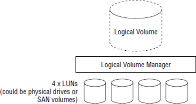
Like other types of snapshots, volume manager snapshots can be used by backup applications: a consistent snapshot of a volume is taken, and it is the consistent snapshot that is backed up. Regarding snapshot technologies, volume manger snapshots sit in the host-based camp, and as a result they consume host resources. They do not offload any of the legwork involved in snapshot management to the storage array.
On the plus side, they can provide filesystem-level consistency and can usually be configured to be read/write snapshots. However, both of these capabilities depend on the volume manager technology in question and sometimes on the Linux kernel in use. It's no more or less complicated than array-based snapshots. Whichever technology you choose, you need to do your research and testing before deploying in your live production environment.
Quite often, in order to make volume manager snapshots application consistent, you need to manually (probably via a script) quiesce your applications.
On the down side, volume manager snapshots often have an associated performance overhead. It is also quite common for volume manager snapshots to be visible and exportable only to the host that is running the volume manager.
They are, however, widely used in smaller shops and development environments.
Summary
In this chapter we discussed how replication technologies fit into the bigger picture of business continuity and disaster recovery, before diving deeper into the different types of replication common in today's storage world. We compared synchronous and asynchronous replication, and the impacts each has on recovery point objectives, application performance, network bandwidth requirement, and other factors. We discussed how replication technologies are implemented at different layers of the stack, including application, operating system, and storage array. We also discussed common replication topologies and how they protect businesses and their data from different types of disaster. We then finished the chapter discussing snapshot technologies and application consistency.
Chapter Essentials
Synchronous Replication Synchronous replication offers zero data loss, giving the best recovery point objective of all the different types of replication. However, it carries a performance penalty that increases as you add distance between your source and target volumes.
Asynchronous Replication Asynchronous replication practically guarantees to lose some of your data. However, it does not impose the performance penalty that synchronous replication does. Asynchronous replication allows you to have your source and target at almost limitless distances from each other and can usually be configured with a recovery point objective.
Application-Layer Replication Replication performed at the application layer levies the burden of replication on the host but offers excellent application awareness, ensuring that remote replicas are transactionally consistent.
Space-Efficient Snapshots Space-efficient snapshots are point-in-time copies of volumes, or virtual machines, that provide an image of a volume, or virtual machine, at a specific time. These can be used as rollback points, sources for backups, or testing. They are absolutely not a replacement for backups!