
Chapter
4
RAID: Keeping Your Data Safe
TOPICS COVERED IN THIS CHAPTER:
- What RAID is and why we need it
- Hardware vs. software RAID
- Striping
- Parity
- Mirroring
- Standard RAID levels
- Performance
- Reliability
- The future of RAID
 This chapter covers all of the RAID material required for the CompTIA Storage+ exam, and more. You'll start with the basics, including a history of RAID technology and why it has been, and continues to be, such a fundamental requirement in enterprise technology across the globe.
This chapter compares different implementations of RAID, including an analysis of both hardware RAID and software RAID, the pros and cons of each, and some potential use cases for both. It also covers the fundamental principles and concepts that comprise most of the RAID implementations commonly seen in the real world, including RAID groups, striping, parity, mirroring, and the commonly implemented RAID levels.
You'll finish the chapter looking at some of the more recent and niched implementations, as well as what the future may hold for this long-standing technology that might be starting to struggle in coping with the demands of the modern world.
The History and Reason for RAID
Back in the day, big expensive computers would have a single, large, expensive drive (SLED) installed. These disk drives
- Were very expensive
- Posed a single point of failure (SPOF)
- Had limited IOPS
RAID was invented to overcome all of these factors.

In 1988, Garth Gibson, David Patterson, and Randy Katz published a paper titled “A Case for Redundant Arrays of Inexpensive Disks (RAID).” This paper outlined the most commonly used RAID levels still in use today and has proven to be the foundation of protecting data against failed disks for over 20 years. As their work was published as a paper and not a patent, it has seen almost universal uptake in the industry and remains fundamental to data protection in data centers across the globe.
Fast forward 25+ years. Disk drives still fail regularly and often without warning. Most large data centers experience multiple failed disk drives each day. And while disk drive capacities have exploded in recent years, performance has not, leading to a disk drive bloat problem, where capacity and performance are severely mismatched—although solid-state media is changing the game here a little. These facts combine and conspire to ensure that RAID technology remains fundamental to the smooth running of data centers across the world.
So, even though RAID technology is over 25 years old, a solid understanding of how it works and protects your data will stand you in good stead throughout your IT career.

RAID is a form of insurance policy for your data, and you do not want to find yourself uninsured in a time of crisis. Yes, RAID has a cost, but that cost is literally pennies when compared to the cost of downtime or application rebuilds. Also, your insurance portfolio for data protection should include far more than just RAID! Your business-critical applications should have multiple levels of protection, including at least the following: RAID, MPIO, replication, and backups.
What Is RAID?
RAID is an acronym. Back in the day it referred to redundant array of inexpensive disks. Nowadays, most folks refer to it as redundant array of independent disks. And with the emergence of solid-state drives, which aren't really disks, maybe it's about to see another change and become redundant array of independent drives.
Anyway, the raison d'etre of RAID technology in the modern IT world is twofold:
- Protect your data from failed drives.
- Improve I/O performance by parallelizing I/O across multiple drives.
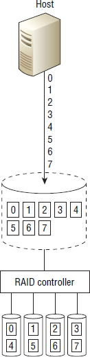
In order to deliver increased performance and protection, RAID technology combines multiple physical drives and creates one or more logical drives that span those multiple physical drives, as shown in Figure 4.1.
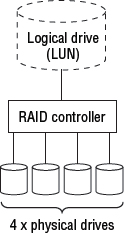
A logical drive can typically be one of two things. It can be a subset of a single physical drive with the intention of creating multiple logical drives—sometimes called partitions—from the single physical drive. Or, as is the case in Figure 4.1, a logical drive can be a device created from capacity that is aggregated from multiple physical drives. Figure 4.1 shows a single logical drive created from capacity on four physical drives. Sometimes a logical drive can be referred to as a logical disk, logical volume, virtual disk, or virtual volume.
There are several RAID levels in wide use today—such as RAID 1, RAID 10, RAID 5, and RAID 6—each of which has its own strengths and weaknesses. You'll look closely at the more popular RAID levels throughout the chapter and consider their strengths and weaknesses, as well as potential use cases. However, before looking closer at RAID levels, let's first look at some of the fundamental concepts and components.

Actually, before we set out, it is of paramount importance to stress the following: RAID is not a backup solution or a replacement for backups! RAID protects data only against disk drive failures and not the many other things that can destroy your data.
Hardware or Software RAID
RAID can be implemented in software or hardware.
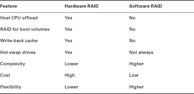
Software RAID is usually implemented as part of the OS, on top of the OS by a logical volume manager such as Linux LVM, or as part of a filesystem as with ZFS. Either way, this results in software RAID using host resources such as CPU and RAM. This is not as much of a problem as it once was, thanks to the monster CPUs and oodles of RAM we commonly see in servers these days. Consumption of host-based resources is not much of a problem if implementing RAID 1 mirroring, but it can become more of an issue when performing parity RAID such as RAID 5 or RAID 6, especially if you have a lot of drives in the RAID set. Also, because the OS needs to be booted before the RAID software can initialize, OS boot volumes cannot be RAID protected with software RAID. Throw into the mix the lack of some of the fringe benefits that typically come with hardware RAID, such as faster write performance and faster rebuilds, and software RAID quickly starts to look like a poor-man's RAID.
Microsoft Storage Spaces
In the Windows Server 2012 operating system, Microsoft has implemented an LVM known as Storage Spaces.
Storage Spaces allows you to pool together heterogeneous drives and create virtual volumes, known as storage spaces, using the capacity in these pools. These storage spaces can optionally be software RAID protected—either mirror protected (RAID 1) or parity protected (RAID 5).
While Storage Spaces is a relatively recent attempt at providing advanced storage features in OS software, its implementation of software RAID still suffers from the same performance
“Microsoft Storage Spaces” was styled runinhead in Word, with runinpara's after it. Seemed intentional, so I steted the change to H2 and removed the bold from the runinparas…was change to H2 correct?
penalties that other software RAID solutions suffer from when it comes to using parity for protection. Also, Storage Spaces offers none of the advanced filesystem and software RAID integration that ZFS does.
While the pooling aspects of Storage Spaces might be good, the software RAID implementation is basic and has not been able to reach escape velocity, remaining grounded to the same performance and usage limitations found in so many other software RAID implementations.
Mirroring, parity, and RAID levels are explained in more detail in the “RAID Concepts” section.
Hardware RAID, on the other hand, sees a physical RAID controller implemented in the server hardware—on the motherboard or as an expansion card—that has its own dedicated CPU and either battery-backed or flash-backed RAM cache. Because of this dedicated hardware, no RAID overhead is placed on the host CPU. Also, because hardware RAID controllers initialize before the OS, this means that boot volumes can be RAID protected. The battery-backed or flash-backed cache on the RAID controller also offers improved write performance via write-back caching—acknowledging the I/O back to the host when it arrives in cache rather than having to wait until it is written to the drives in the RAID set. One potential downside to hardware RAID controllers inside servers is that they provide a SPOF. Lose the RAID controller, and you lose your RAID set. Despite this, if you can afford it, most people find that they go with hardware RAID most of the time.
Table 4.1 highlights the pros and cons of hardware and software RAID.
External RAID controllers, such as storage arrays, are also forms of hardware RAID. Storage arrays usually have several advantages over and above stand-alone hardware RAID controllers that are typically installed in server hardware. These advantages include the following:
- Redundancy. RAID controllers installed on server motherboards or as PCIe cards are single points of failure. While it is true that storage arrays can themselves be single points of failure, they tend to be extremely highly available, and it is rare that they catastrophically fail.
- Storage arrays offer larger caches, so they can often achieve higher performance.
- Storage arrays support multiple drive types. Internal RAID controllers tend not to allow you to mix and match drives.
- Storage arrays support many more drives for both capacity and increasing performance through parallelization.
- Storage arrays usually offer advanced features such as snapshots, replication, thin provisioning, and so forth.
Microsoft Storage Spaces—Software RAID
In the Windows Server 2012 operating system, Microsoft has implemented an LVM known as Storage Spaces.
Storage Spaces allows you to pool together heterogeneous drives and create virtual volumes, known as storage spaces, using the capacity in these pools. These storage spaces can optionally be software RAID protected—either mirror protected (RAID 1) or parity protected (RAID 5).
While Storage Spaces is a relatively recent attempt at providing advanced storage features in OS software, its implementation of software RAID still suffers from the same performance penalties that other software RAID solutions suffer from when it comes to using parity for protection. Also, Storage Spaces offers none of the advanced filesystem and software RAID integration that ZFS does.
While the pooling aspects of Storage Spaces might be good, the software RAID implementation is basic and has not been able to reach escape velocity, remaining grounded to the same performance and usage limitations found in so many other software RAID implementations.
RAID Concepts
Let's tackle the major concepts that comprise most RAID technologies. A solid understanding of these concepts is vital to a full understanding of RAID technologies and the impact they will have on your data availability and performance.
RAID Groups
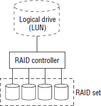
RAID groups, also known as RAID sets or RAID arrays, is the term used to refer to a group of drives that are combined and configured to work together to provide increased capacity, increased performance, and increased reliability. All drives in a RAID group are connected to the same RAID controller and are owned by that RAID controller. Figure 4.2 shows a RAID set containing four drives that has been configured as a single logical drive.
It is also possible to configure more than one logical volume per RAID set. Figure 4.3 shows the same four-disk RAID set, but this time configured as two logical drives of differing sizes.
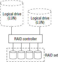
Drives in a RAID set are sometimes referred to as members.
Striping
The process of creating a logical drive/logical volume that is spread across all the drives in a RAID set is known as striping. The idea behind striping is to parallelize I/O across as many drives as possible in order to get the performance of every drive. Every write to a logical drive that is striped across all drives in a RAID set gets distributed across all the drives in the RAID set, potentially giving it access to all of the IOPS and MB/sec of every drive.
Figure 4.4 shows I/O from a host being written to a logical volume that is striped over four physical drives. If each physical drive is capable of 200 IOPS, the potential performance from the logical volume is 800 IOPs. If the volume was not striped, but instead confined entirely to a single drive, it could perform at only 200 IOPS.
Striping is a technique that is fundamental to many RAID algorithms for both performance and reliability reasons.
The process of striping a logical drive over multiple physical drives also allows the logical drive to access all the capacity available on each physical drive. For example, a logical volume created on a simple RAID set containing four 900 GB drives could be as large as 3,600 GB. Thus, striping also allows for increased capacity as well as performance.
Parity
Parity is a technique used in RAID algorithms to increase the resiliency, sometimes referred to as fault tolerance, of a RAID set.
Parity-based RAID algorithms reserve a percentage of the capacity of the RAID set (typically one or two drives’ worth) to store parity data that enables the RAID set to recover from certain failure conditions, such as failed drives.
Let's look at a quick and simple example of how parity works to protect and reconstruct binary data. Parity can be either even or odd parity, and it doesn't matter which of the two is employed, as they both achieve the same end goal: providing fault tolerance to binary data sets. Let's use odd parity in our examples. Odd parity works by making sure that there is always an odd number of ones (1s) in a binary sequence. Let's assume all of our binary sequences comprise four bits of data, such as 0000, 0001, 1111, and so on. Now let's add an extra bit of data after the fourth bit, and use this extra bit as our parity bit. As we are using odd parity, we will use this bit to ensure that there is always an odd number of 1s in our five bits of data. Let's look at a few examples:
00001—The fifth bit of data (our parity bit) is a 1 so that there is an odd number (one) of 1s in our data set.
01110—This time we make the fifth bit of data a 0, to ensure there are an odd number of 1s (three) in the data set.
10000—This time we make the parity bit a 0 so that there is an odd number of 1s (one) in the data set. If we'd made it a 1, there would have been two 1s in the data set.
All well and good, but how does this make our data set fault tolerant? First up, as we've added only a single parity bit, our data set can tolerate the loss of only a single bit of data, but that lost bit can be any bit in the data set. Anyway, to see how it works, let's look at our three example data sets again, only this time we've removed a bit of data and will use the principle of odd parity to determine and reconstruct that missing bit of data.
0_001—As we are using odd parity, our missing bit must be a 0. Otherwise, we would have an even number of 1s in the data set.
011_0—This time we know that the missing bit is a 1. If it was a 0, we would have an even number of 1s in our data set.
1000_—This time we've lost the parity bit. But this makes no difference. We can still apply the same logic and determine that we are missing a 0.
As our example data set has five bits of data but contains only four bits of real user data—one bit is parity overhead—we have lost one bit, or 20 percent. Put in other terms, our data set is 80 percent efficient, as 80 percent of the bits are used for real data, with 20 percent used to provide fault tolerance. And it may be useful to know that at the low level, parity is computing using an exclusive OR (XOR) operation, although knowledge of this won't help you in your day-to-day job.
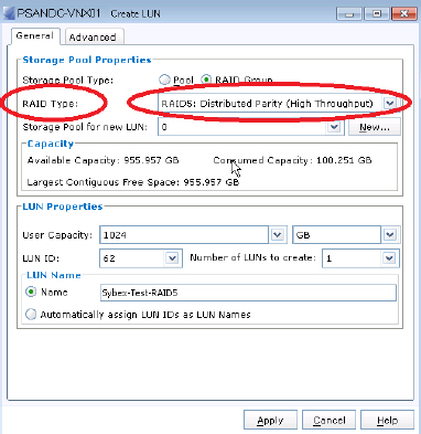
Figure 4.5 shows the option to configure a RAID 5 volume on an EMC VNX array. As you can see, the GUI used to create the volume doesn't ask anything about XOR calculations or other RAID internals.
How much parity is set aside for data protection, and the overall fault tolerance of the RAID set, depends on the RAID level employed. For example, RAID 5 can tolerate a single drive failure, whereas RAID 6 can tolerate two drive failures. We will discuss these in more detail shortly.
Figure 4.6 shows a single drive in a five-drive RAID set being reserved for parity data. In this example, the usable capacity of the RAID set is reduced by 20 percent. This RAID set can also tolerate a single drive failure.
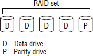
Figure 4.7 shows the same five-drive RAID set after experiencing single and double drive failures.
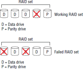
If the RAID set in Figure 4.7 had contained two parity drives (higher fault tolerance), it would have survived the double drive failure scenario. However, the second parity drive would have reduced the usable capacity of the RAID set from 80 percent to 60 percent.
Parity is usually computed via exclusive OR (XOR) calculations, and it doesn't really matter whether your RAID controller works with odd or even parity—so long as it works it out properly.
Parity-based RAID schemes can suffer performance impact when subject to high write workloads, especially high write workloads composed of small-block random writes. This is known as the write penalty, which we discuss in detail later. When it comes to high read workloads, parity-based RAID schemes perform well.
RAID Stripes and Stripe Sizes
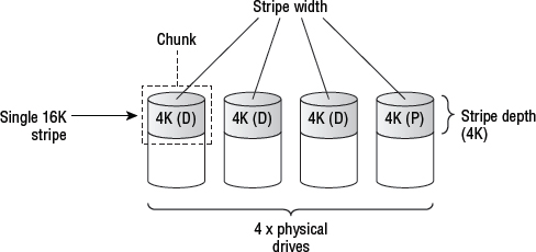
All forms of traditional RAID that employ striping and parity work on the basis of stripes. Stripes are made from a row of chunks. The size of these chunks determines the stripe depth and stripe size, while the number of members in the RAID set determines the stripe width. I think we need a diagram!
Figure 4.8 shows a four-drive RAID set configured as RAID 5 (3+1) and has explanations for each of the elements that make up the stripe.
Now for a few quick principles and a bit of lingo that apply to most traditional RAID sets.
Stripes are made up of chunks from each drive in the RAID set. Each chunk is made from contiguous blocks in a single physical drive. All chunks in a RAID configuration are of equal size—usually a multiple of the drive's sector size—and this size is known as the stripe depth. Stripe width is equal to the number of drives in the RAID set. The RAID set in Figure 4.8 has the following characteristics:
- Stripe depth is 4 KB. This is because each chunk is 4 KB, and the chunk size is equal to the stripe depth.
- Stripe size is 16 KB. Four 4 KB chunks.
- Stripe width is 4. There are four members in the RAID set.
When a host writes to a volume on a RAID controller, the RAID controller writes this data out in stripes so that it touches all drives in the RAID set. For example, if a host writes 24 KB to the RAID set in Figure 4.8, the RAID controller will write this out as two stripes. This is because each stripe has 12 KB of usable data and 4 KB of parity. As it writes this data out in stripes, it writes 4 KB to drive 0, before switching to drive 1, where it writes the next 4 KB, and so on. Writing 24 KB to this RAID set will require two rows, or stripes.
Storage arrays—themselves RAID controllers—tend to have far larger stripe sizes than host-based RAID controllers. It is not uncommon for a storage array to have a chunk size of 64 KB, 128 KB, or 256 KB. If the storage array has a chunk size of 256 KB, then a RAID 5 (3+1) would have a stripe size of 1,024 KB. The larger stripe sizes seen in storage arrays tend to be aligned to the slot size of the array's cache.
Chunk Size and Performance
The following can be used as a guiding principle that will work in most situations: If your I/O size will be large, you want to go with a smaller chunk size. If your I/O size will be small, you want larger chunks.
So, what constitutes a small or a large chunk size? Generally, small chunks can range from as small as 512 bytes to maybe 4 KB or 8 KB. Anything larger than that is starting to get into the realms of larger chunks.
Small I/O and Large Chunks
Small I/Os, such as 4 KB I/Os common in database environments, tend to work a lot better with larger chunk sizes. The objective here is to have each drive in the RAID set busy working and seeking independently on separate I/Os—a technique known as overlapping I/O.
If you have a larger chunk size with small I/O, you can easily incur increased positional latency. That is, while the heads on one drive might have arrived in position and be ready to service its portion of the I/O, the heads on the other drives in the RAID set might not yet have arrived in position, meaning that you have to wait until the heads on all drives in the RAID set arrive in place before the I/O can be returned. And if you subject your RAID controller to lots of small-block random I/O with a large chunk size, this can take its toll and reduce performance.
Large I/O and Small Chunks
Low I/O environments that work with large files often benefit from a smaller stripe size, as this allows each large file to span all physical drives in the RAID set. This approach enables each file to be accessed far more quickly, involving every drive in the RAID set to read or write the file. This configuration is not conducive to overlapping I/O, as all drives in the array will be used for reading or writing the single large file.
Common use cases for small chunk sizes include applications that access large audio/video files or scientific imaging applications that often manipulate large files.
Mixed Workloads
Fortunately, the default setting on most RAID controllers is usually good enough and designed for mixed workloads. It is recommended to change the defaults only if you know what you are doing and know what your workload characteristics will be. If you don't know either, don't mess with the chunk and stripe size. Also most storage arrays don't let you fiddle with this, as it is tightly aligned to cache slot size and other array internals.
Hot-Spares and Rebuilding
Some RAID arrays contain a spare drive that is referred to as a hot-spare or an online spare. This hot-spare operates in standby mode—usually powered on but not in use—during normal operating circumstances, but it is automatically brought into action, by the RAID controller, in the event of a failed drive. For example, a system with six drives could be configured as RAID 5 (4+1) with the remaining drive used as a hot-spare.
The major principle behind having hot-spares is to enable RAID sets to start rebuilding as soon as possible. For example, say your RAID set encounters a failed drive at 2 a.m., and nobody is on site to replace the failed drive. If it has a hot-spare, it can automatically start the rebuild process and be back on the road to recovery by the time you arrive at work in the morning. Obviously, larger disk drives take longer to rebuild, and in today's world, where drives are in excess of 4 TB, these could take days to rebuild.
The process of rebuilding to a hot-spare drive is often referred to as sparing out.
Hot-spares are not so common in host-based RAID controllers but are practically mandatory in storage arrays, with large storage arrays often containing multiple hot-spare drives.
Distributed Sparing and Spare Space
Some modern storage arrays don't actually contain physical hot-spare drives. Instead, they reserve a small amount of space on each drive in the array and set this space aside to be used in the event of drive failures. This is sometimes referred to as distributed sparing. For example, a storage array with 100 1 TB drives might reserve ∼2 GB of space on each drive as spare space to be used in the event of drive failures. This space will be deducted from the overall usable capacity of the array.
This amount of reserved spare space is the equivalent of two 1 TB drives, meaning the array has the equivalent of two spare drives. In the event of a drive failure, the array will rebuild the contents of the failed drive to the spare space on every surviving drive in the array. This approach has the advantage of knowing that the drives that the spare space are on are in working condition. Having dedicated spare drives that are used only in the event of drive failures is prone to the hot-spare itself failing when needed most. Also of significance is that all the drives in the system are available all the time, increasing system performance and allowing RAID rebuilds to be distributed across all drives, making rebuild operations faster and lowering the performance impact.
Of course, this example was hugely oversimplified, but serves to explain the principle.
Rebuilding tends to be accomplished by one of two methods:
- Drive copy, used when rebuilding in mirrored sets such as RAID 1
- Correction copy/parity rebuild, used when rebuilding sets based on parity protection
Performance Impact of Rebuilds
Drive copy rebuilds are computationally simple compared to parity rebuilds, meaning they are far faster than having to reconstruct from parity.
RAID 1 mirror sets always recover with a drive copy, but parity-based RAID schemes such as RAID 5 and RAID 6 usually have to recover data via a parity rebuild.
Let's look at drive copy rebuilds and parity rebuilds:
- Drive copy operations are the preferred rebuild method but can be performed only if a drive is proactively failed by the RAID controller. This means that the drive has not actually failed yet, but the drive thresholds that the RAID controller monitors indicate that a failure is about to occur. This is known as a predictive failure. Drive copy rebuilds place additional stress on only the failing drive and the hot-spare.
- Parity rebuilds are the absolute last line of defense once a drive in a parity set has actually failed. These are computationally more intensive than drive copies and place additional load on all drives in the RAID set including the hot-spare—all surviving drives are read from stripe 0 through to the last stripe, and for each stripe, the missing data is reconstructed from by parity via exclusive OR (XOR) calculations. This additional load on the surviving drives in the RAID set is sometimes blamed when a second drive fails during the parity rebuild.
This point about additional load being blamed on second drive failures is potentially significant. During a rebuild operation, additional load is placed on all drives in the RAID set. It is entirely possible that this additional load can cause other drives in the RAID set to fail. This risk is being addressed by some of the more modern RAID implementations.
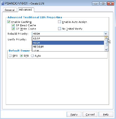
RAID Rebuild Priorities
Also, many RAID controllers, including storage arrays, allow you to prioritize the rebuild process. Giving rebuilds a lower priority leads to longer rebuilds, whereas giving rebuilds a high priority can have an impact on user I/O for the duration of the rebuild operation.
If you have large pools or single-parity RAID, you may wish to increase the priority of the rebuild so that your window of exposure to a second drive failure is decreased. In contrast, if you employ dual-parity RAID, you may feel more comfortable lowering the priority of the rebuild in the knowledge that you can safely suffer a second drive failure without losing data.
Figure 4.9 shows a screenshot of an EMC CLARiiON array showing available options for rebuild priority.
Rebuild Domains and Blast Zones
When rebuilding a failed drive in a RAID set, the RAID set is usually the rebuild domain. This means that all the rebuild activity and overhead is placed on the drives within the RAID set. Similarly, the blast zone refers to the area of impact when data is lost from a failed RAID set (such as a double drive failure in a RAID 5 set). When using traditional RAID sets, the blast zone is just the failed RAID set and any volumes using that RAID set. However, in more-modern arrays that implement storage pools comprising multiple RAID sets, a failed RAID set can cause data loss on every volume in the pool that the RAID set is associated with, dramatically increasing the size of the blast zone.
RAID Controllers
A RAID controller can be either software or hardware. Software RAID controllers are exactly that, software, and are often implemented via a logical volume manager. Hardware RAID controllers, on the other hand, are dedicated hardware designed specifically for performing RAID and volume management functions.
Hardware RAID controllers come in two major flavors:
- Internal
- External
As previously mentioned, hardware RAID controllers are dedicated hardware, either on the motherboard or as a PCIe card, that offload all RAID functions from the host CPU and RAM. These RAID functions include creating logical disks (referred to in SCSI parlance as logical units and usually abbreviated as LUN), striping, mirroring, parity calculation, rebuilding, hot-spares, and caching.
Write-Back Caching on Internal RAID Controllers
Most internal RAID controllers have an onboard DRAM/NVRAM cache used to speed up reads and writes. However, in order to safely speed up writes, a RAID controller must be able to protect its cache from losing data in the event of a low of power. There are two common approaches to this with modern RAID controllers:
Battery-Backed Caching In battery-backed caching, a small battery or capacitor (SuperCap) is placed on the RAID controller card and used to maintain power to the DRAM cache so that its contents are not lost when the power fails. However, power must be restored before the battery runs out. Otherwise, the data will still be lost.
Flash-Backed Caching In flash-backed caching, a battery or SuperCap is placed on the RAID controller card and used to power the DRAM cache long enough to copy its contents to flash memory so that its contents are preserved.
Battery-backed write-back caching (BBWC) is losing popularity in the wake of flash-backed caches. However, they still exist.
Caching technology is like oxygen to the storage industry. Starve a storage solution of cache, and its performance will drop like a stone. The benefits of placing a cache in front of spinning disks is covered in several chapters throughout this book, but caching also has a positive benefit in RAID systems. Any RAID controller, or storage array, that caches all inbound writes should be able to avoid the parity overhead of most writes under normal operating circumstances. This is done by holding small writes in cache and coalescing them into larger full-stripe writes (FSWs), where the overhead for parity computation is negligible.
RAID Levels
This section covers the most common RAID levels seen in the real world: RAID 0, RAID 1, RAID 10, RAID 5, and RAID 6. We'll also explore the less commonly used RAID levels.
RAID 0
First and foremost, there is nothing redundant about RAID 0! This means it provides no protection for your data. No parity. No mirroring. Nothing. Nada!
If I could recommend one thing about RAID 0, it would be never to use it. While some folks might come up with niche configurations where it might have a place, I'd far rather play it safe and avoid it like the plague.
However, in case it comes up on an exam or a TV quiz show, we'll give it a few lines.
RAID 0 is striping without parity. The striping means that data is spread over all the drives in the RAID set, yielding parallelism. More disks = more performance. Also, the lack of parity means that none of the capacity is lost to parity. But that is not a good thing. The lack of parity makes RAID 0 a toxic technology that is certain to burn you if you use it.
RAID 0 Cost and Overhead
There is no RAID overhead with RAID 0, as no capacity is utilized for mirroring or parity. There is also no performance overhead, as there are no parity calculations to perform. So, RAID 0 is nothing but good news on the cost and performance front. However, it is a ticking time bomb on the resiliency front.
Use Cases for RAID 0
Potential use cases for RAID 0 include the following:
- If you want to lose data
- If you want to lose your job
- If your data is 100 percent scratch, losing it is not a problem, and you need as much capacity out of your drives as possible
- As long as there is some other form of data protection such as network RAID or a replica copy that can be used in the event that you lose data in your RAID 0 set
- If you want to create a striped logical volume on top of volumes that are already RAID protected
Options 1 and 2 are not recommended.
Option 3 is a potential poisoned chalice. Far too many systems start out their existence being only for testing purposes and then suddenly find that they are mission critical. And you do not want anything mission critical built on the sandy foundation of RAID 0.
Option 4 is more plausible but could also end up being a poisoned chalice. When data is lost, people always look for somebody else to blame. You could find the finger of blame being pointed at you.
Option 5 is quite common in the Linux world, where the LVM volume manager is well-known and very popular. However, it is absolutely vital that the underlying volume supporting the RAID 0 striped volume is RAID protected. Exercise 4.1 walks you through an example of creating a striped volume (RAID 0) with Linux LVM.
EXERCISE 4.1
Creating a Striped Volume with Linux LVM
Assume that you have a Linux host with four 100 GB volumes that are RAID 6 volumes: sda, sdb, sdc, and sdd. You will create a single striped volume (RAID 0) on top of these four RAID 6 volumes. Follow these steps:
- Run the pvcreate command on all four of the RAID 6 volumes. Be careful, because doing this will destroy any data already on these volumes.
- Now you'll create a volume group called vg_sybex_striped using your four volumes that you just ran the pvcreate commands against.
# vgcreate vg_sybex_striped /dev/sda /dev/sdb /dev/sdc /dev/sdd
- Once the volume group is created, run a vgdisplay command to make sure that the volume group configuration has been applied and looks correct.
  #  vgdisplay
  --- Volume Group ---
VG Name               vg_sybex_striped
VG Access             read/write
VG Status             available/resizable
VG #                  2
<output truncated>
- Once you have confirmed that the volume group configuration is as expected, run the following lvcreate command to create a single 200 GB logical volume.
# lvcreate -i4 -I4 -L 200G -n lv_sybex_test_vol vg_sybex_striped
The -i option ensures that the logical volume will use all four physical volumes you created with the pvcreate command. The -I option specifies a 4 KB stripe size. The -L command specifies a size of 200 GB.
You now have a 200 GB RAID 0 (striped) logical volume that is sitting on top of four 100 GB RAID 6 volumes. These RAID 6 volumes are SAN-presented volumes, meaning that the RAID 6 protection is being provided by the storage array. Also, you have ∼200 GB of free space in the volume group, which you can use to create more logical volumes or to expand your existing logical volume in the future.
What Happens When a Drive Fails in a RAID 0 Set
You lose data.
End of story. You will possibly face the end of employment in your current role. You won't need to worry about performance degradation or rebuild times. Neither will be happening. If you are lucky, you will have a remote replica or backup to enable some form of recovery.
Figure 4.10 shows the career-limiting RAID 0.
![]() Real World Scenario
Real World Scenario
RAID 0 Does Not Protect Your Data!
A company lost data when a RAID 0 volume failed. This data had to be recovered from backup tapes based on a backup taken nearly 24 hours earlier. The administrator responsible for the storage array insisted he had not created any RAID 0 volumes and that there must be a problem with the array. The vendor analyzed logs from the array and proved that the administrator had indeed created several RAID 0 volumes. The logs even showed the dates on which the volumes were created and had recorded the administrator's responses to warnings that RAID 0 volumes would lose data if any drive failed. Needless to say, the administrator did not last long at the company.
RAID 1
RAID 1 is mirroring. A typical RAID 1 set comprises two disks—one a copy of the other. These two disks are often referred to as a mirrored pair. As a write comes into the RAID controller, it is written to both disks in the mirrored pair. At all times, both disks in the mirror are exactly up-to-date and in sync with each other. All writes to a RAID 1 volume are written to both disks in the RAID set. If this is not possible, the RAID set is marked as degraded.
Degraded mode refers to the state of a RAID set when one or more members (drives) of the set is failed. The term degraded refers to both degraded redundancy and degraded performance. In degraded mode, a RAID set will continue to service I/O; it will just be at greater risk of losing data should another drive fail, and performance may be impeded by data having to be reconstructed from parity. The latter is not the case for RAID 1, which does not use parity. However, even in a RAID 1 set, read performance may be degraded as the read can no longer be serviced from either disk in the mirrored pair.
A RAID 1 set contains a minimum of two drives. As the term mirroring suggests, one drive is a mirror copy of the other. This configuration is often written as RAID 1 (1+1). The 1+1 refers to one drive for the primary copy and one drive for the mirrored copy. If either of the drives in the RAID set fails, the other can be used to service both reads and writes. If both drives fail, the data in the RAID set will be lost.
RAID 1 is considered a high-performance and safe RAID level. It's considered high performance because the act of mirroring writes is computationally lightweight when compared with parity-based RAID. It is considered safe because rebuild times can be relatively fast. This is because a full copy of the data still exists on the surviving member, and the RAID set can be rebuilt via a fast drive copy rather than a slower parity rebuild.
All good.
Exercise 4.2 shows how to create a mirrored logical volume with Linux LVM.
EXERCISE 4.2
Creating a Mirrored Logical Volume with Linux LVM
Let's assume you have a Linux host that is already presented with two 250 GB volumes that are not RAID protected. These could be SAN volumes or locally attached DAS drives: sda and sdb. Now let's form these two volumes into a mirrored logical volume (RAID 1).
- Run the pvcreate command on both of the 250 GB volumes (sda and sdb). This is a destructive process that will destroy any data already on the devices.
# pvcreate /dev/sda
# pvcreate /dev/sdb
- Now create a volume group called vg_sybex_mirrored by using your two volumes that you just ran the pvcreate commands against.
# vgcreate vg_sybex_mirrored /dev/sda /dev/sdb
- Once the volume group is created, run a vgdisplay command to make sure that the volume group configuration has been applied and looks correct.
  # vgdisplay
  --- Volume Group ---
VG Name               vg_sybex_mirror
VG Access             read/write
VG Status             available/resizable
VG #                  1
<output truncated>
- Once it is confirmed that the volume group configuration is as expected, run the following lvcreate command to create a single 200 GB mirrored logical volume.
# lvcreate -L 200G -m1 -n lv_sybex_mirror_vol vg_sybex_mirrored
The -L command specifies a size of 200 GB. It is worth noting that the 200 GB mirrored logical volume will not consume all the capacity of the volume group you created. This is fine.
You now have a 200 GB RAID 1 (mirrored) logical volume that is sitting on top of two 250 GB devices.
RAID 1 Cost and Overhead
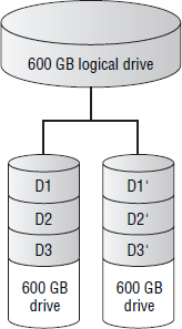
The downside to RAID 1—and it's only a downside to the storage administrator and the cost center owner who owns the storage budget—is that RAID 1 sacrifices a lot of capacity on the altar of protection. All RAID 1 configurations use 50 percent of total physical capacity to provide the protective mirror. This sacrificed capacity is referred to as RAID overhead.
Also, say we assume a capital expenditure (cap-ex) cost of $5,000 per terabyte and you need to purchase 32 TB. On the face of it, this might sound like $160,000. However, if this needs to be RAID 1 protected, you need to buy double the raw capacity, which will obviously double the cap-ex cost from $160,000 to $320,000. That hurts!
For this reason, RAID 1 tends to be used sparingly—no pun intended.
Figure 4.11 shows two 600 GB drives in a RAID 1 set. Although the resulting logical drive is only 600 GB, it is actually consuming all the available space in the RAID set because this is a RAID 1 set and therefore loses half of its physical raw capacity to RAID overhead.
Use Cases for RAID 1
If you don't keep a tight rein on it, everybody will be asking for RAID 1. Database Administrators (DBAs) are especially guilty of this, as they have all been indoctrinated with anti–RAID 5 propaganda. If they insist on RAID 1, ask them to put their money where their mouth is and cross-charge them.
RAID 1 is an all-around good performer but excels in the following areas:
- Random write performance. This is because there is no write penalty for small random writes as there is with RAID 5 and RAID 6 (more on this later).
- Read performance. Depending on how your RAID controller implements RAID 1, read requests can be satisfied from either drive in the mirrored pair. This means that for read performance, you have all of the IOPS from both drives. Not all RAID controllers implement this.
What Happens When a Drive Fails
When a drive fails in a RAID 1 set, the set is marked as degraded, but all read/write operations continue. Read performance may be impacted.
Once the failed drive is replaced with a new drive or a hot-spare kicks in, the RAID set will be rebuilt via a drive copy operation whereby all the contents of the surviving drive are copied to the new drive. Once this drive copy operation completes, the RAID set is said to be back to full redundancy.
RAID 10
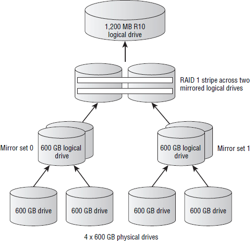
RAID 1+0, often referred to as RAID 10, and pronounced RAID ten, is a hybrid of RAID 1 (mirror sets) and RAID 0 (stripe sets). The aim is to achieve the best of both worlds. And generally speaking, it works exactly like that.
Let's look at how a RAID 10 set is created. Assume we have four 600 GB drives and we want to create a RAID 10 set. We take the first two drives and create a mirrored pair from them. Then we take the last two drives and make a separate mirrored pair from them. This gives us two logical 600 GB drives, each of which is RAID 1 protected. The next step is then to take these two 600 GB RAID 1–protected drives and create a stripe set across them. The stripe set doesn't add any mirroring or parity, so no additional capacity is lost. All it does is increase performance by striping data over more drives. The net result now is 1,200 GB of capacity that is both mirrored and striped.
The Point of RAID 10
The thinking behind RAID 10 is pretty straightforward: to get the protection and performance of RAID 1 and turbo boost it with an additional layer of striping. That striping adds more drives to the RAID set, and drives = IOPS and MB/sec!
So, as long as you can afford the capacity overhead that comes with any derivative of RAID 1, then RAID 10 potentially offers the best mix of performance and protection available from the traditional RAID levels.
Figure 4.12 shows graphically how a RAID 10 set is created, and Exercise 4.3 walks us through the high level process of creating one.
EXERCISE 4.3
Creating a RAID 10 RAID Set
Your RAID controller will do this for you, so this is purely conceptual. Let's assume you have four 1 TB physical drives in your server/storage array. To create a RAID 10 set, follow these steps:
- Use two of the drives to create a 1 TB mirrored volume.
- Do exactly the same with the remaining two drives. At the end of these two steps, you would have two 1 TB mirrored volumes.
- Take these two mirrored volumes and create a single 2 TB RAID 0 striped volume across them.
The end result would be a single 2 TB volume that is protected with RAID 1 and has the added performance benefit of all reads and writes being striped across the drives.
Beware of RAID 01
RAID 10 and RAID 01 are not the same, and people often get the two mixed up. You always want RAID 10 rather than RAID 01. The technical difference is that RAID 01 first creates two stripe sets and then creates a mirror between them. The major concern with RAID 01 is that it is more prone to data loss than RAID 10. Some RAID controllers will automatically build a RAID 10 set even if they call it RAID 1.
RAID 5
Despite its critics, RAID 5 probably remains the most commonly deployed RAID level—although most people consider it a best practice to use RAID 6 for all drives that are 1 TB or larger.
RAID 5 is known technically as block-level striping with distributed parity. This tells us two things:
Block level tells us that it is not bit or byte level. Block size is arbitrary and maps to the chunk size we explained when discussing striping.
Distributed parity tells us that there is no single drive in the RAID set designated as a parity drive. Instead, parity is spread over all the drives in the RAID set.
RAID 5 Cost and Overhead
Even though there is no dedicated parity drive in a RAID 5 set, RAID 5 always reserves the equivalent of one disk worth of blocks, across all drives in the RAID set, for parity. This enables a RAID 5 set—no matter how many members are in the set—to suffer a single drive loss without losing data. However, if your RAID 5 set loses a second drive before the first is rebuilt, the RAID set will fail and you will lose data. For this reason, you will want your RAID 5 sets to have fast rebuild times.
Common RAID 5 configurations include the following:
- RAID 5 (3+1)
- RAID 5 (7+1)
RAID Notation
Let's take a quick look at common RAID notation. When writing out a RAID set configuration, the following notation is commonly used:
RAID X (D+P)
X refers to the RAID level, such as 1, 5, or 6.
D indicates the number of data blocks per stripe.
P indicates the number of parity blocks per stripe.
So if our RAID set has the equivalent of three data drives and one parity drive, this would make it a RAID 5 set, and we would write it as follows: RAID 5 (3+1).
As the rules of RAID 5 state only that it is distributed block-level parity, it is possible to have RAID 5 sets containing a lot more drives than the preceding examples—for example, RAID 5 (14+1). However, despite the number of drives in a RAID 5 set, as always, only a single drive failure can be tolerated without losing data.
The amount of capacity lost to parity in a RAID 5 set depends on how many data blocks there are per parity stripe. The calculation is parity/data ×![]() 100 expressed as a percentage.
100 expressed as a percentage.
So, in our RAID 5 (3+1) set, we lose 25 percent of capacity to parity, as 1/4 × 100 = 25. A RAID 5 (7+1) set is more space efficient in that it sacrifices only 12.5 percent of total space to parity: 1/8 × 100 = 12.5. And at a far extreme, RAID 5 (15+1) sacrifices only 6.25 percent of space to parity.
Be careful, though. While RAID 5 (15+1) yields a lot more usable space than RAID 5 (3+1), there are two drawbacks:
- Longer rebuilds. Rebuild times for the 15+1 RAID set will be longer than the 3+1 set because the XOR calculation will take longer, and there are more drives to read when reconstructing the data.
- Lower performance, because it's harder to create FSWs and avoid the RAID 5 write penalty. We will discuss this shortly.
What Happens When a Drive Fails in a RAID 5 Set
When a drive fails in a RAID 5 set, you have not lost any data. However, you need the RAID set to rebuild as quickly as possible, because while there is a failed drive in your RAID set, it is operating in degraded mode. The performance of the RAID set and its ability to sustain drive failure are degraded. So it's a good idea to get out of degraded mode as quickly as possible.
Assuming there is a hot-spare available, the RAID controller can immediately start rebuilding the set. This is achieved by performing exclusive OR (XOR) operations against the surviving data in the set. The XOR operation effectively tells the RAID controller what was on the failed drive, enabling the hot-spare drive to be populated with what was on the failed drive. Once the rebuild completes, the RAID set is no longer in degraded mode, and you can relax.
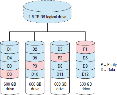
Figure 4.13 shows a RAID 5 (3+1) array.
RAID 5 Write Penalty
Parity-based RAID schemes, such as RAID 5 and RAID 6, suffer from an inherent performance defect known as the write penalty. This is especially a problem in situations where there is high write activity, particularly high random write activity. It occurs because calculating parity for small-block writes incurs additional I/O on the backend as follows. A small-block random write to a RAID 5 group incurs four I/Os for each write:
Let's look at a quick example. Figure 4.13 shows a simplified RAID 5 (3+1) RAID set. Let's assume we wanted to write only to block D1 on row 0. To calculate the new parity for row 0, the RAID controller will have to read the existing data, read the existing parity, write the new data to D1, and write the new parity to P1. This overhead is a real pain in the neck and can trash the performance of the RAID set if you subject it to high volumes of small-block writes. For this reason, many application owners, especially DBAs, have an aversion to RAID 5. However, many RAID 5 implementations go a long way in attempting to mitigate this issue.
Full Stripe Writes Do Not Suffer from the Write Penalty
Because the write penalty applies to only small-block writes, where the write size is smaller than the stripe size of the RAID set, performing larger writes avoids this problem. This can be achieved via caching.
By putting a large-enough cache in front of a RAID controller, the RAID controller is able store up small writes and bundle them together into larger writes. This is a technique called write coalescing. The aim is to always write a full stripe—because writing a full stripe does not require additional operations to read blocks that you are not writing to, and you can write the data and parity in a single operation.
However, write coalescing is a feature of high-end external RAID controllers (storage arrays) and is an advanced technique. It is not usually a feature of a hardware RAID controller in a server, and certainly not a technique used by software RAID controllers. The effectiveness of write coalescing can also be diminished if the RAID controller is subject to particularly high write workloads.
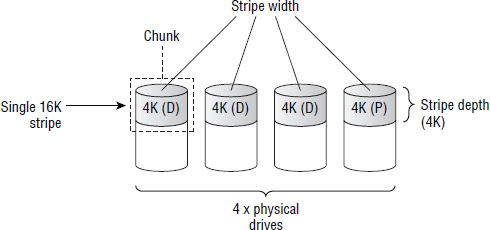
Distributed RAID Schemes May Limit the Impact of the Write Penalty
Distributed RAID refers to the ability to spread a RAID-protected volume over hundreds of drives, with each successive stripe existing on a separate set of drives.
Figure 4.14 shows a traditional four-drive RAID group. In this figure, four consecutive stripes in a logical volume are shown.
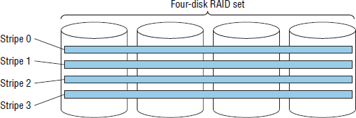
Figure 4.15 shows the same four stripes for the same logical volume, but this time spread across all 16 drives in a 16-drive pool.
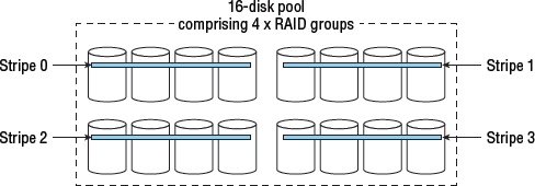
While the configuration in Figure 4.15 doesn't avoid the write penalty, it can offset some of the impact by using all 16 drives in parallel and potentially writing multiple stripes in parallel.
The write penalty affects only parity-based RAID systems and does not afflict RAID 1 or RAID 0. It is most noticeable when experiencing high-write workloads, particularly high-random-write workloads with a small block-size.
RAID 6
RAID 6 is similar to RAID 5. Both do block-level striping with distributed parity. But instead of single parity, RAID 6 employs double parity. This use of double parity brings some clear-cut pros and cons.
RAID 6 is based on polynomial erasure codes. You will look at erasure codes later in the chapter as they may prove to be instrumental in the future of RAID and data protection, especially in cloud-based architectures.
RAID 6 Cost and Overhead
As with RAID 5, there is no dedicated parity drive in a RAID 6 set. The parity is distributed across all members of the RAID set. However, whereas RAID 5 always reserves the equivalent of one drive's worth of blocks for parity, RAID 6 reserves two drives’ worth of blocks for two discrete sets of parity. This enables a RAID 6 set—no matter how many members are in the set—to suffer two failed drives without losing data. This makes RAID 6 an extremely safe RAID level!
Common RAID 6 configurations include the following:
- RAID 6 (6+2)
- RAID 6 (14+2)
The same as with RAID 5, a RAID 6 set can have an arbitrary number of members, but it always has two sets of discrete parity! So RAID 6 (30+2) is a valid RAID 6 configuration, so long as your RAID controller supports it and you have enough drives in the set.
The amount of capacity lost to RAID overhead in a RAID 6 set abides by the same rules as RAID 5. You divide 2 by the total number of drives in the set and then multiply that number by 100, as shown here:
- RAID 6 (14+2): 2/16 × 100 = 12.5 percent capacity overhead. This is sometimes referred to as 87.5 percent efficient.
- RAID 6 (30+2): 2/32 × 100 = 6.25 percent capacity overhead, or 93.75 percent efficient.
As with RAID 5, the more drives in the set, the slower the rebuild and the lower the write performance. Remember, parity-based RAID schemes suffer the write penalty when performing small-block writes. These can be offset by using cache to coalesce writes and perform full-stripe writes. However, the larger the RAID set (actually the larger the stripe size), the harder it is to coalesce enough writes to form a full-stripe write.
When to Use RAID 6
On the positive side, RAID 6 is rightly considered extremely safe. It can suffer two drive failures in the set without losing data. This makes it an ideal choice for use with large drives or for use in pools with large numbers of drives.
Large drives tend to be slow drives—in terms of revolutions per minute (RPM)—and therefore take a lot longer to rebuild than smaller, faster drives. For this reason, the window of exposure to a second drive failure while you are performing a rebuild is greatly increased. RAID 6 gives you an extra safety net here by allowing you to suffer a second drive failure without losing data. Also if you are deploying pools with hundreds of drives, if you were to lose a RAID set making up that pool, you could punch a hole in every volume using the pool. That would mean data loss on every volume using the pool! So for these two use cases, RAID 6 is very much the de facto choice.
RAID 6 performs well in high-read situations.
When to Not Use RAID 6
The major downside of RAID 6 is performance, especially performance of small-block writes in an environment experiencing a high number of writes. Because RAID 6 doubles the amount of parity per RAID stripe, RAID 6 suffers more severely from the write penalty than RAID 5. The four I/Os per small-block write for a RAID 5 set becomes six I/Os per write for a RAID 6 set. Therefore, RAID 6 is not recommended for small-block-intensive I/O requirements, and in the vast majority of cases, it is not used for any heavy write-based workloads.
Another area where RAID 6 suffers is in usable capacity. This is because RAID 6 has two parity blocks per stripe. However, this can be offset by deploying RAID 6 in large RAID sets such as RAID 6 (6+2) or quite commonly RAID 6 (14+2). These lose 25 percent and 12.5 percent, respectively. Don't forget, though, the larger your stripe size, the harder it is for the RAID controller to coalesce writes in cache for full-stripe writes.
When all is said and done, RAID 6 is rightly viewed as a slow, but safe, RAID choice. It is almost always the RAID level of choice for RAID groups containing drives over 1 TB in size.
![]() Real World Scenario
Real World Scenario
RAID 6: A Safe Pair of Hands
A company suffered more than 30 failed drives in a single storage array over a period of less than a week—due to a bug with a specific batch of disk drives from a particular vendor. However, this company was employing large drive pools and therefore had deployed RAID 6. Despite losing so many drives in such a short period of time, no triple drive failures occurred in a single RAID set making up the pool, so no data was lost!
Less Commonly Used RAID Levels
Some RAID levels are not as commonly used as the previously discussed RAID levels. Even so, it is important for you to understand what these RAID levels are. RAID 2, RAID 3, and RAID 4 are briefly introduced here.
RAID 2
RAID 2 is bit-level striping and is the only RAID that can recover from single-bit errors. As it is not used in the real world, this is as much as you will need to know about it.
RAID 3
RAID 3 performs parity at the byte level and uses a dedicated parity drive. RAID 3 is extremely rare in the real world.
RAID 4
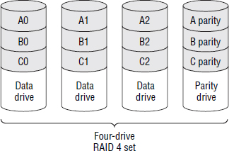
RAID 4 is similar to RAID 5. It performs block-level striping but has a dedicated parity drive.
One of the common issues with using dedicated parity drives is that the parity drive can become a bottleneck for write performance. Figure 4.16 shows a four-disk RAID 4 set with a dedicated parity drive. In this RAID configuration, each time you update just a single block on each row, you have to update the parity on the dedicated parity drive. This can cause the parity drive to become a bottleneck.
However, it has the advantage that the RAID set can be easily expanded by adding more disks to the set and requiring only the parity drive to be rebuilt. Other RAID schemes with distributed parity would require the entire RAID set to be rebuilt when adding drives.
RAID 4 is more common than RAID 2 and RAID 3 but is nowhere near as popular as RAID 5 and RAID 6.
NetApp's Data ONTAP supports RAID 4 and tightly integrates it with the Write Anywhere File Layout (WAFL) filesystem that is also part of Data ONTAP. By integrating the filesystem and the RAID, as long as the system is nearing capacity and being pushed to the limits, Data ONTAP is able to coalesce writes and avoid the performance impact of the dedicated parity drive (where the parity drive is hit harder than the other drives in the RAID set). Integrating filesystems and RAID schemes can have interesting benefits, which are covered at the end of the chapter when we discuss ZFS.
The Future of RAID
RAID technology has been around for decades. And it's fair to say that while most things in the technology world have moved on enormously in the past two decades, most implementations of RAID have not. Also, the disk drive bloat problem—drives getting bigger and bigger but not faster—is leading to longer and longer rebuild times. And longer rebuild times means you are exposed to the risks of additional drive failures for longer periods of time. This has led to the point we are at now, where traditional approaches to RAID just aren't up to the challenge of today's business and IT demands.
Fortunately, some interesting and important new RAID techniques and technologies have started cropping up. Some of the most popular include those that implement forms of parallel, or distributed, RAID. We will cover a few of these new approaches and technologies that highlight some of the advances made.
As we review some of these modern approaches to RAID, we will reference some vendor-specific technologies. As we do this, the objective isn't to promote or denounce any specific technology. Our interest is purely in looking academically at some of the ways they differ from the traditional approaches and how they attempt to address today's requirements.
IBM XIV and RAID-X
IBM XIV storage arrays implement a form of RAID 1 technology referred to as RAID-X. The reason we are interested in RAID-X is that it is not any kind of RAID 1 your grandmother will recognize. Yes, it loses 50 percent capacity to protection, and yes, it is susceptible to double drive failures. But this is 21st-century, turbo-charged, object-based, distributed RAID. So there are lots of cool things for us to look at.
Object-Based RAID
Object based means that RAID protection is based on objects rather than entire drives. XIV's implementation of object-based RAID is based on 1 MB extents that it refers to as partitions. Each volume on an XIV is made up of multiple 1 MB extents, and it is these 1 MB extents that are RAID-X protected.
However, as all volumes on an XIV are natively thin provisioned, extents are allocated to volumes on demand as data is written to volumes. Interestingly, this leads to improved reprotect and rebuild operations when a drive fails, which we will cover shortly.
Distributed RAID
The object-based nature of RAID-X enables the 1 MB extents that make up RAID-X volumes to be spread out across the entire backend of the XIV array—hundreds of drives. This wide-striping of volumes across the entire backend leads to massively parallel reads, writes, and reprotect operations. This is totally different from the two-drive RAID 1 configurations you looked at earlier!
RAID-X and Reprotecting
RAID-X is susceptible to double drive failures. If a drive in an XIV fails and then a second drive fails before the reprotect operation for the first failure completes, the system will lose data. And because every XIV volume is spread over pretty much every drive on the backend, the blast zone of a double drive failure is immense. It could punch a small hole in every volume on the system—oh, dear! However, and this is significant, RAID-X is highly optimized to reprotect itself blazingly fast! It does this via massively parallel reprotection operations. Let's take a look.
With traditional drive-based approaches to RAID, when a drive fails and the RAID set goes into degraded mode, the only way to get the RAID set back to fully protected mode is to rebuild the contents of the failed drive to another drive—usually to a hot-spare. Drive rebuild operations can take serious amounts of time in the world of multi-TB drives. We're talking days to rebuild large drives on some arrays. Hence the recommendation is to use RAID 6 with large, slow drives. Traditional drive-based RAID also rebuilds entire drives even if there is only a tiny amount of data on the drives. RAID-X is altogether more intelligent.
Another reason double protection is recommended for large drives is that the chances of hitting an unrecoverable read error while performing the rebuild are greatly increased. If you have only single protection for large drives, and during a rebuild you encounter an unrecoverable read error, this can be effectively the same as a second drive failure, and you will lose data. So at least double protection is highly recommended as drives get bigger and bigger.
RAID-X Massively Parallel Rebuilds
When a drive fails in an XIV, RAID-X does not attempt to rebuild the failed drive, at least not just yet. Instead it spends its energy in reprotecting the affected data. This is significant.
Let's assume we have a failed 2 TB drive that is currently 50 percent used. When this drive fails, it will leave behind 1 TB of data spread over the rest of the backend that is now unprotected. This unprotected 1 TB is still intact, but each of those 1,024 1 MB extents no longer has a mirrored copy elsewhere on the array. And because this 1 TB of unprotected data is spread across all drives on the backend, the failure of any other drive will cause some of these unprotected 1 MB extents to be lost. So, in order to reprotect these 1 MB extents as fast possible, the XIV reads each extent from all drives on the backend, and writes new mirror copies of them to other drives spread across the entire backend—all in parallel. Of course, RAID-X makes sure that the primary and mirror copy of any of the 1 MB extents is never on the same drive, and it goes further to ensure that they are also on separate nodes/shelves.
This is an excellent example of a massively parallel many-to-many operation that will complete in just a few short minutes. It is rare to see a drive rebuild operation on an XIV last more than 20–30 minutes, and often they complete much quicker. The speed of the reprotect operation is vital to the viability of RAID-X at such large scale, as it massively reduces the window of vulnerability to a second simultaneous drive failure.
Also, unlike traditional RAID, the parallel nature of a RAID-X rebuild means that it avoids the increased load stress that is typically placed on all disks in the RAID set during normal RAID rebuild operations. In most XIV configurations, each drive shoulders a tiny ~1 percent of the rebuild heavy lifting.
RAID-X and Object-Based Rebuilds
Also, because RAID-X is object based, it reprotects only actual data. In our example of a 2 TB drive that is 50 percent full, only 1 TB of data needs reprotecting and rebuilding. Non-object-based RAID schemes will often waste time rebuilding tracks that have no data on them. By reprotecting only data, RAID-X speeds up reprotect operations.
Once the data is reprotected, RAID-X will proceed to rebuild the failed drive. This rebuild is a many-to-one operation, with the new drive being the bottleneck.
RAID-X on IBM XIV isn't the only implementation of modern object-based parallel RAID, but it is a well-known and well-debated example.
On the topic of object-based rebuilds, other storage arrays such as HP 3PAR, Dell Compellent, and XIO also employ this approach. However, these technologies use object-based RAID with parity and double parity rather than XIV's form of object based mirroring. As the technologies that employ object-based approaches to RAID are all modern arrays, this is clearly the next step in RAID technology.
RAID-X, as well as almost all pool-based backend designs, increases the potential blast zone when double drive failures occur. Because all volumes are spread over all (actually most) drives on the backend, a double drive failure has the potential to punch a small whole in most, if not all, volumes. This is something to beware of and is a major reason that most conventional arrays recommend RAID 6 when deploying large pools. The idea is to reduce risk, and RAID-X does this by its super-fast massively parallel reprotect operations.
ZFS and RAID-Z
RAID-Z is a parity-based RAID scheme that is tightly integrated with the ZFS filesystem. It offers single, double, and triple parity options and uses a dynamic stripe width. This dynamic, variable-sized stripe width is powerful, effectively enabling every RAID-Z write to be a full-stripe write—with the exception of small writes that are usually mirrored. This is brilliant from a performance perspective, meaning that RAID-Z rarely, if ever, suffers from the read-modify-write penalty that traditional parity-based RAID schemes are subject to when performing small-block writes.
RAID-Z volumes are able to perform full-stripe writes for all writes by combining variable stripe width with the redirect-on-write nature of the ZFS filesystem. Redirect-on-write means that data is never updated in place, even if you are updating existing data. Instead, data is always written to a fresh, new location—as a full-stripe write of variable size—and the pointer table is updated to reflect the new location of the updated data, and the old data is marked as no longer in use. This mode of operation results in excellent performance, but begins to tail off significantly when free space starts to get low.
Recovery with RAID-Z
RAID-Z rebuilds are significantly more complex than typical parity-based rebuilds where simple XOR calculations are performed against each RAID stripe. Because of the variable size of RAID-Z stripes, RAID-Z needs to query the ZFS filesystem to obtain information about the RAID-Z layout. This can cause longer rebuild times if the pool is near capacity or busy. On a positive note, because RAID-Z and the ZFS filesystem talk to each other, rebuild operations rebuild only actual data and do not waste time rebuilding empty blocks.
Also, because of the integration of RAID-Z and ZFS, data is protected from silent corruption. Each time data is read, it is passed through a checksum (that was created the last time the data was updated) and reconstructed if the validation fails. This is something that block-based RAID schemes without filesystem knowledge cannot do.
RAID-TM
RAID-TM is a triple-mirror-based RAID. Instead of keeping two copies of data as in RAID 1 mirror sets, RAID-TM keeps three copies. As such, it loses 2/3 of capacity to protection but provides good performance and excellent protection if you can get past the initial shock of being able to use only 1/3 of the capacity you purchased.
RAID 7
The idea behind RAID 7 is to take RAID 6 one step further by adding a third set of parity. At first glance, this seems an abomination, but its inception is borne out of a genuine need to protect data on increasingly larger and larger drives. For example, it won't be long before drives are so large and slow that it will take a full day to read them from start to finish, never mind rebuild them from parity! And as we keep stressing, longer rebuilds lead to larger windows of exposure, as well as the likelihood of encountering an unrecoverable read error during the rebuild.
RAIN
RAIN is an acronym for redundant/reliable array of inexpensive nodes. It is a form of network-based fault tolerance, where nodes are the basic unit of protection rather than drives or extents. RAIN-based approaches to fault tolerance are increasingly popular in scale-out filesystems, object-based storage, and cloud-based technologies. RAIN-based approaches to fault tolerance are covered in other chapters where we talk about scale-out architectures, object storage and cloud storage.
Erasure Codes
Erasure codes is another technology that is starting to muscle its way into the storage world. More properly known as forward error correction (FEC) or sometimes information dispersal algorithms (IDA), this technology has been around for a long time and is widely used in the telco industry. Also, erasure codes are already used in RAID 6 technologies as well some consumer electronics technologies such as CDs and DVDs. And let's face it, any data protection and recovery technology that can still produce sounds from CDs after my children have had their hands on them must surely have something to offer the world of enterprise storage!
Whereas parity schemes tend to work well at the disk-drive level, erasure codes initially seem to be a better fit at the node level, protecting data across nodes rather than drives. They can, and already are, used to protect data across multiple nodes that are geographically dispersed. This makes them ideal for modern cloud-scale technologies.
Erasure codes also work slightly differently from parity. While parity separates the parity (correction codes) from the data, erasure codes expand the data blocks so that they include both real data and correction codes. Similar to RAID, erasure codes offer varying levels of protection, each of which has similar trade-offs between protection, performance, and usable capacity. As an example, the following protection levels might be offered using erasure code technology:
- 9/11
- 6/12
In the first example, the data can be reconstructed if only 9 out of the 11 data blocks remain, whereas 6/12 can reconstruct data if only 6 of 12 data blocks remain. 6/12 is obviously similar to RAID 1 in usable capacity.
While erasure codes are the foundation of RAID 6 and are finding their way into mass storage for backup and archive use cases, it is likely that they will become more and more integral to protection of primary storage in the enterprise storage world, and especially cloud-based solutions.
Finally, current implementations of erasure codes don't perform particularly well with small writes, meaning that if erasure codes do form the basis of data protection in the future, it is likely that we will see them used in cloud designs and maybe also in large scaleout filesystems, with more-traditional RAID approaches continuing to protect smaller-scale systems and systems that produce small writes, such as databases.
Chapter Essentials
The Importance of RAID RAID technologies remain integral to the smooth operation of data centers across the world. RAID can protect your data against drive failures and can improve performance.
Hardware or Software RAID Hardware RAID tends to be the choice that most people go for if they can afford it. It can offer increased performance, faster rebuilds, and hot-spares, and can protect OS boot volumes. However, software RAID tends to be more flexible and cheaper.
Stripe Size and Performance Most of the time, the default stripe size on your RAID controller will suffice—and often storage arrays will not let you change it. However, if you know your workloads will be predominantly small block, you should opt for a large stripe size. If you know your I/O size will be large, you should opt for a smaller stripe size.
RAID 1 Mirroring RAID 1 offers good performance but comes with a 50 percent RAID capacity overhead. It's a great choice for small-block random workloads and does not suffer from the write penalty.
RAID 5 RAID 5 is block-level interleaved parity, whereby a single parity block per stripe is rotated among all drives in the RAID set. RAID 5 can tolerate a single drive failure and suffers from the write penalty when performing small-block writes.
RAID 6 RAID 6 is block-level interleaved parity, whereby two discrete parity blocks per stripe are rotated among all drives in the RAID set. RAID 6 can tolerate a two-drive failure and suffers from the write penalty when performing small-block writes.
Summary
In this chapter we covered all of the common RAID level in use today, including those required for the CompTIA Storage+ exam. As part of our coverage, we looked at the various protection and performance characteristics that each RAID level provides, as well as cost and overheads for each. We also addressed some of the challenges that traditional RAID levels face in the modern IT world, and mentioned some potential futures for RAID.