Chapter
10

Capacity Optimization Technologies

TOPICS COVERED IN THIS CHAPTER:

• Thin provisioning
• Overprovisioning
• Data compression
• Data deduplication
• Auto-tiering
• Sub-LUN auto-tiering

Over the past few years, the storage industry has seen a major uptick in the turnout of high-quality capacity optimization technologies. These include thin provisioning, compression, deduplication, and auto-tiering. This trend is due to several factors, including shrinking IT budgets, the need to do more with less, the natural maturation of storage technologies, and a major push from flash storage vendors that need strong capacity optimization technologies in order to make their offerings price-competitive with solutions based on spinning disk. The net result is that there are a whole host of high-quality capacity optimization technologies to choose from.

This chapter presents all of these major capacity optimization technologies. It covers topics such as inline and post-process data deduplication and data compression, as well as thin provisioning, overprovisioning, and tiering. Following our usual approach, you'll dig deep into how these technologies work and are implemented in the real world, as well as mapping some of the technologies to use cases, such as backup and archiving, and primary storage. You'll learn where some of these technologies might not be the best fit, so you don't make mistakes that you could have avoided. The chapter discusses the impacts that capacity optimization technologies have on key principles such as performance, availability, and cost. After reading this chapter, you should be equipped to deploy the right data-efficiency technologies in the right places.

Capacity Optimization Technologies Overview

SNIA uses the term capacity optimization methods to refer to all methods used to reduce the space required to store persistent data. This pretty much puts it in a nutshell. Capacity optimization technologies are all about doing more with less: storing more data on less hardware, sweating your storage assets, managing data growth, squeezing every inch of capacity out of media, and the list could go on.

While there may be some other fringe benefits, such as performance improvements, these are very much side-benefits and bonuses. The raison d'etre of capacity optimization technologies is increasing capacity utilization and enabling you to store more data in less space.

When discussing increasing capacity utilization, we'll naturally discuss the technologies that will have a positive impact on financial matters such as return on investment (ROI) and total cost of ownership (TCO). This includes things such as $/TB acquisition cost; reduced data center footprint; reduced network bandwidth (network costs); reduced power and cooling; and a leaner, greener data center.

Performance Implications

Let's take a quick moment to look at some potential performance implications that result from implementing capacity optimization technologies. As with most technologies, capacity optimization technologies can increase or decrease overall storage and system performance. For example, tiering (which we will consider to be a capacity optimization technology) might move data down to lower tiers, decreasing performance, or up to higher tiers, increasing performance. Deduplication similarly can increase or decrease performance. Inline deduplication of data residing on primary storage arrays that are based on spinning disk will usually lower both read and write performance, whereas post-process deduplication of virtual machines with a sizable read cache can significantly improve performance. Thin provisioning (TP) can also improve performance by scattering data over very large numbers of drives on the backend of a storage array, but it can also lead to fragmented layout on the backend and negatively impact sequential performance.

We'll cover plenty on the topic of performance as we discuss each capacity optimization technology, but for now the takeaway point should be that capacity optimization technologies can send performance in either direction—up or down. It all depends on how the technology is implemented. So beware.

Types of Capacity Optimization Technologies

Lots of capacity optimization technologies are available—in fact, so many that it can be confusing. To clarify, let's begin with a quick overview of the types of technology, which you'll explore more throughout the chapter:

There are also various places at which capacity optimization technologies can be implemented: source-based, appliance-based, gateways, target-based, and so on. They can also be implemented inline, post-process, or even somewhere in between. We'll cover most of these options throughout the chapter.

Use Cases for Capacity Optimization Technologies

The use cases for capacity optimization technologies are almost limitless. Technologies that were once considered off-limits because of performance and other overhead are now becoming viable thanks to advances in CPU, solid-state storage, and other technologies.

Over the next few years, we will see capacity optimization technologies implemented at just about every level of the stack and included in most mainstream storage technologies. Backup, archiving, primary storage, replication, snapshots, cloud, you name it, if it's not already there, it will be soon.

There is a lot to cover, so let's press on.

Thin Provisioning

In the storage world, thin provisioning (TP) is a relatively new technology but one that has been enthusiastically accepted and widely adopted. A major reason behind the rapid adoption of TP is that it helps save money, or at least avoid spending it. It does this by working on an allocate-on-demand model, in which storage is allocated to a volume only when data is actually written, rather than allocating large quantities of storage up front. You'll look more closely at how it works shortly.

This chapter uses the terms thick volumes and thin volumes, but these concepts are also known as traditional volumes and virtual volumes.

Thick Volumes

As thick volumes are the oldest and most common type of volumes, let's take a moment to review them to set the scene for our discussion on the more recent and complicated topic of thin volumes.

Thick volumes are simple. You choose a size, and the volume immediately reserves/consumes the entire amount defined by the size. Let's say you create a 1 TB thick volume from an array that has 10 TB of free space. That thick volume will immediately consume 1 TB and reduce the free capacity on the array to 9 TB, even without you writing any data to it. It is simple to understand and simple to implement, but it is a real waste of space if you never bother writing any data to that 1 TB thick volume. In a world with an insatiable appetite for a finite pool of storage, such potential wasting of space is a problem—and it's the main problem with thick volumes that can't go unaddressed.

The problem of thick volumes allowing users to waste storage space is only compounded by the common practice of people wildly overestimating the amount of storage they need, just in case they may need it at some point in the future. It's common for storage arrays to be fully provisioned—with all their capacity carved up into thick volumes and presented out to hosts—but for a lot less than half of that capacity to be actually used by the hosts. The other half sits there doing nothing. Imagine a 200 TB storage array that has all 200 TB allocated to hosts as thick volumes, but the total combined data from all hosts written to those thick volumes being in the region of 80 TB. That's wasting more than 100 TB of storage. That kind of ratio of provisioned-to-used capacity is still common in too many places. However, thanks in no small part to thin provisioning, this is becoming less of an issue.

Thin Volumes

Thin volumes work a lot differently than thick volumes. Thin volumes consume little or sometimes no capacity when initially created. They start consuming space only as data is written to them.

Let's take a quick look at how a 1 TB thin volume works. When we create this 1 TB thin volume, it initially consumes little or no space. If the host that we export it to never writes to it, it will never consume any more space. Let's say an eager developer thinks her new business application needs a new volume to cope with the large amounts of data it will generate and requests a 2 TB volume. As a storage administrator, you allocate a new 2 TB volume from your array that has 10 TB of free space available. However, the application generates only a maximum of 200 GB of data, nowhere near the amount of data expected. If this 2 TB volume had been a thick volume, the instant you created it, it would have reduced your array's available capacity from 10 TB to 8 TB. Most of that would have been wasted, as the application never even comes close to touching the sides of the 2 TB volume. However, as it was a thin volume, only 200 GB was ever written to it. The unused 1.8 TB of space is still available to the array to allocate to other volumes. This is obviously a powerful concept.

An important concept to understand when it comes to thin provisioning is extent size. Extent size is the unit of growth applied to a thin volume as data is written to it.

For example, say a system has a TP extent size of 768 KB. Each time a host writes any data to an unused area of the TP volume, space will be allocated to the TP volume in multiples of 768 KB. The same would be true if the extent size was 42 MB; any time data is written to a new area of the TP volume, a 42 MB extent would be allocated to the volume. If your host has written only 4 KB of data to the TP volume, a 42 MB extent might seem a bit like overkill, and certainly from a capacity perspective, very large extent sizes are less efficient than small extent sizes. However, smaller extent sizes can have a performance overhead associated with them, because the system has to perform more extent allocations as data is written to a volume. Say a host writes 8 MB of data to a new TP volume. If the extent size was 42 MB, the system would have to allocate only a single extent, whereas if the extent size were 768 KB, it would have to allocate 11 extents, which is potentially 11 times as much work. In most situations, the capacity-related benefits of smaller extent sizes are seen as being more significant than the potential performance overhead of working with smaller extent sizes, because in the real world any potential performance overhead is so small that it's rarely, if ever, noticed.

Sometimes you might hear TP extents referred to as pages.

Overprovisioning

Most thin provisioning–based storage arrays allow an administrator to overprovision the array. Let's take a look at an example that explains how overprovisioning works and what its pros and cons are.

Let's start with a thin provisioning storage array that has 100 TB of physical capacity (after RAID overhead and so on) and 50 attached hosts. Now let's assume that the total amount of storage capacity provisioned to these 50 hosts totals 150 TB. Obviously, these volumes have to be thin provisioned. If they weren't, the maximum amount of capacity that could be provisioned from the array would be 100 TB. But because we've provisioned out 150 TB of capacity, and the array has only 100 TB of real physical capacity installed, we have overprovisioned our array. In overprovisioning terms, this array is 50 percent overprovisioned, or 150 percent provisioned.

There are some obvious benefits to overprovisioning, but there are some drawbacks, too.

Overprovisioning allows an array to pretend it has more capacity than it does. This allows improved efficiency in capacity utilization. In our previous example, the array had 100 TB of physical usable storage and was overprovisioned by 50 percent. This array could still be heavily underutilized. It is entirely possible that although having provisioned out 150 TB to connected hosts, these hosts may have written only 60 TB to 70 TB of data to the array.

Now, let's assume the $/TB cost for storage on that array was $2,000/TB, meaning the array cost $200,000. If we had thickly provisioned the array, it would have been able to provision only 100 TB of capacity. In order to cater for the additional 50 TB requested, we would have had to buy at least 50 TB more capacity, at a cost of $100,000. However, because the array was thinly provisioned, we were able to overprovision it for zero cost to handle the additional requirement of 50 TB. So there are clear financial benefits to overprovisioning.

However, on the downside, overprovisioning introduces the risk that your array will run out of capacity and not be able to satisfy the storage demands of attached hosts. For example, say our array has only 100 TB of physical usable storage, and we've provisioned out 150 TB. If the attached hosts demand over 100 TB of storage, the array will not be able to satisfy that. As a result, hosts will not be able to write to new areas of volumes, which may cause hosts and applications to crash. You don't want this scenario to happen, and avoiding it requires careful planning and foresight. Overprovisioning should be done only if you have the tools and historical numbers available to be able to trend your capacity usage. You should also be aware of the kind of lead time required for you to be able to get a purchase order approved and your vendor to supply additional capacity. If it takes a long time for your company to sign off on purchases and it also takes your vendor a long time to ship new capacity, you will need to factor that into your overprovisioning policy.

Because of the risks just mentioned, it's imperative that the people ultimately responsible for the IT service be aware of and agree to the risks. That said, if managed well, overprovisioning can be useful and is becoming more and more common in the real world.

Trending

As I've mentioned the importance of trending in an environment that overprovisions arrays, let's take a moment to look at some of the metrics that are important to trend. This list is by no means exhaustive, but it covers metrics that are commonly trended by storage administrators who overprovision:

• Physical usable capacity
• Provisioned/allocated capacity
• Used capacity

As part of your trending, you will want to be tracking these metrics at least monthly. Figure 10.1 shows an example chart that has tracked the metrics for the past 16 months and has added a trend line predicting how used capacity is expected to increase over the next 6 months.

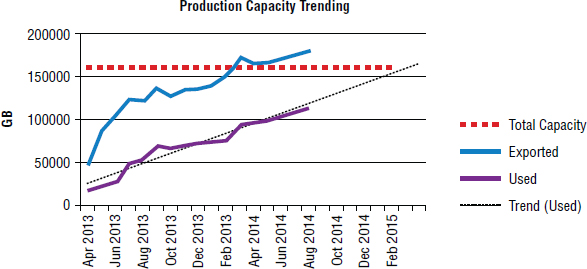
As you can see, the array in Figure 10.1 will break the bank (used capacity will exceed physical usable capacity) somewhere around February 2015. Of course, you will want additional capacity to be installed into the array by November 2014. Graphs and trending charts like these are vital in all overprovisioning environments. Share them with management on a regular basis. Print them out, laminate them, and pin them on your desk so you don't ignore them!

Trigger Points for Purchase Orders

If you plan to overprovision in your environment, you will need to identify trigger points for new capacity purchases. These trigger points are conditions that cause you to purchase new capacity.

A common trigger point is based on used capacity. For example, you may have a trigger point that states that as soon as used capacity reaches 90 percent of physical usable capacity, you start ordering more storage. If you were using 90 percent capacity as a trigger point and you had an array with 200 TB of physical usable storage, you would start the process for installing new capacity as soon as used capacity reaches 180 TB.

It is vital that you don't wait until it's too late to get more capacity. The process of installing new capacity can be quite long in some organizations. You might include obtaining formal quotes, raising a purchase order (PO), following a PO sign-off process, placing the order and PO with the vendor, waiting for parts delivery, waiting for parts installation, and so on.

Following are three of the most common trigger points used by most organizations:

• Available unused capacity
• Percentage of available capacity
• Percentage overprovisioned

There are several reasons for choosing different trigger metrics or even utilizing more than one trigger. For example, 20 TB of free space might work well for a medium-sized array that has up to 200 TB of physical usable storage. 20 TB is 10 percent of a 200 TB array. However, if your array has 800 TB of usable physical storage, 20 TB is all of a sudden a mere 2.5 percent of total array capacity. And larger arrays tend to have more hosts attached and therefore grow faster than smaller arrays, meaning that 20 TB might last a while on a small array with a handful off hosts attached, but it won't last as long on a large array with hundreds of hosts attached.

Space Reclamation

Despite the huge benefits of thin provisioning, over time thin volumes get less and less thin, which is called bloat. Without a way to remove the bloat, you'd eventually get to a position where your thin volumes used up all of their possible space, making them little better than thick volumes. This is where space reclamation comes to the rescue, by giving us a mechanism to keep thin volumes thin.

One of the main reasons for bloat is that most traditional filesystems don't understand thin provisioning and don't inform storage arrays when they delete data. Let's look at a quick example. Assume a 100 GB filesystem on a 100 GB thin provisioned volume. If the host writes 90 GB of data to the filesystem, the array sees this and allocates 90 GB of data to the volume. If the host then deletes 80 GB of data, the filesystem will show 10 GB of used data and 90 GB of available space. However, the array has no knowledge that the host has just deleted 80 GB of data, and will still show the thin volume as 90 percent used. This bloat is far from ideal.

Now let's look at how space reclaim helps avoid this scenario.

Zero Space Reclamation

Space reclamation—often referred to as zero space reclamation or zero page reclamation—is a technology that recognizes deleted data and can release the extents that host the deleted data back to the free pool on the array, where they can be used for space for other volumes.

Traditional Space Reclamation

In the past, operating systems and filesystems were lazy when it came to deleting data. Instead of zeroing out the space where the deleted data used to be, the filesystem just marked the area as deleted, but left the data there. That's good from the operating system's perspective because it's less work than actually zeroing out data and it makes recovering deleted data a whole lot easier. However, it's no use to a thin provisioning storage array. As far as the array knows, the data is still there. In these situations, special tools or scripts are required that write binary zeros to the disk so that the array can then recognize the space as deleted and reclaim it for use elsewhere.

Once binary zeros were written to the deleted areas of the filesystem, the array would either dynamically recognize these zeros and free up the space within the array, or you would need an administrator to manually run a space reclamation job on the array. Both approaches result in the same outcome—increased free space on the array—but one required administrative intervention and the other didn't.

Reclaiming zero space on a host isn't too difficult. Exercise 10.1 walks you through how to do this.

The UNMAP SCSI Standard

If all of this seems like a lot of work to free up space, you're right, especially in a large environment with thousands of hosts. Fortunately, a much slicker approach exists. Most modern operating systems include filesystems that are designed to work in conjunction with array-based thin provisioning.

T10 (a technical committee within the INCITS standards body responsible for SCSI standards) has developed a SCSI standard referred to as UNMAP, which is designed specifically to allow hosts and storage arrays to communicate information related to thin provisioning with each other. For example, when a host operating system deletes data from a filesystem, it issues SCSI UNMAP commands to the array, informing it of the extents that have been deleted. The array can then act on this data and release those extents from the volume and place them back in the array-free pool where they can be used by other hosts. This is way easier than having to manually run scripts to write zeros!

Fortunately, most modern operating systems, such as RHEL 6, Windows 2012, and ESXi 5.x, ship with thin provisioning–friendly filesystems and implement T10 UNMAP.

Inline Space Reclamation

As previously mentioned, some storage arrays are able to watch for incoming streams of binary zeros and do either of the following:

• Not write them to disk if they are targeted at new extents in the volume (the host may be performing a full format on the volume)
• Release the extents they are targeted to if the extents are already allocated (the host is running a zero space reclaim script)

This is a form of inline space reclamation. It can usually be enabled and disabled only by a storage administrator because it has the potential to impact performance.

Older arrays tend to require an administrator to manually run space reclamation jobs to free up space that has been zeroed out on the host. This is a form of post-process reclamation. Although both approaches work, the inline approach is far simpler from an administration perspective.

Thin Provisioning Concerns

As with most things in life, there's no perfect solution that works for everything, and thin provisioning is no different. Although it brings a lot of benefits to the table, it also has one or two things you need to be careful about:

• Heavily sequential read workloads can suffer poor performance compared to thick volumes.
• There is the potential for a small write performance overhead each time new space is allocated to a thin volume.

As I keep mentioning, if you do plan to overprovision, make sure you keep your trending and forecasting charts up-to-date. Otherwise, you risk running out of space and causing havoc across your estate.

Be warned: overprovisioning does not simplify capacity management or storage administration. It makes it harder, and it adds pressure on you as a storage administrator. To gain the potential benefits, thin provisioning and overprovisioning require some effort.

Compression

Compression is a capacity optimization technology that enables you to store more data by using less storage capacity. For example, a 10 MB PowerPoint presentation may compress down to 5 MB, allowing you to store that 10 MB presentation using only 5 MB of disk space. Compression also allows you to transmit data over networks quicker while consuming less bandwidth. All in all, it is a good capacity optimization technology.

Compression is often file based, and many people are familiar with technologies such as WinZip, which allows you to compress and decompress individual files and folders and is especially useful for transferring large files over communications networks. Other types of compression include filesystem compression, storage array–based compression, and backup compression. Filesystem compression works by compressing all files written to a filesystem. Storage array–based compression works by compressing all data written to volumes in the storage array. And backup compression works by compressing data that is being backed up or written to tape.

There are two major types of compression:

• Lossless compression
• Lossy compression

As each name suggests, no information is lost with lossless compression, whereas some information is lost with lossy compression. You may well be wondering how lossy compression could be useful if it loses information. One popular form of lossy compression is JPEG image compression. Most people are familiar with JPEG images, yet none of us consider them poor-quality images, despite the fact that JPEG images have been compressed with a lossy compression algorithm. Lossy compression technologies like these work by removing detail that will not affect the overall quality of the data. (In the case of JPEGs, this is the overall quality of the image.) It is common for the human eye not to be able to recognize the difference between a compressed and noncompressed image file, even though the compressed image has lost a lot of the detail. The human eye and brain just don't notice the difference. Of course, lossy compression isn't ideal for everything. For example, you certainly wouldn't want to lose any zeros before the decimal point on your bank balance—unless, of course, your balance happens to be in the red!

How Compression Works

Compression works by reducing the number of bytes in a file or data stream, and it's able to do this because most files and data streams repeat the same data patterns over and over again. Compression works by re-encoding data so that the resulting data uses fewer bits than the source data.

A simple example is a graphic that has a large, blue square in the corner. In the file, this area of blue could be defined as follows:

A simple compression algorithm would take this repeating pattern and change it to something like the following:

This is much shorter but tells us the same thing without losing data (thus being lossless). All we have done is identified a pattern and re-encoded that pattern into something else that tells us exactly the same thing. We haven't lost anything in our compression, but the file takes up fewer bits and bytes.

Of course, this is only an example to illustrate the point. In reality, compression algorithms are far more advanced than this.

Compression of primary storage hasn't really taken the world by storm. It exists and has some use cases, but its uptake has been slow to say the least.

Performance is the main reason that compression of primary storage hasn't taken the world by storm. Some compression technologies have the unwanted side-effect of reducing storage performance. However, if done properly, compression can improve performance on both spinning disk and solid-state media. Performance is important in the world of primary storage, so it's important to be careful before deploying compression technologies in your estate. Make sure you test it, and be sure to involve database administrators, Windows and Linux administrators, and maybe even developers.

Beyond primary storage, compression is extremely popular in the backup and archive space.

There are two common approaches to array-based compression (for primary storage as well as backup and archive):

• Inline
• Post-process

Let's take a look at both.

Inline Compression

Inline compression compresses data while in cache, before it gets sent to disk. This can consume CPU and cache resources, and if you happen to be experiencing particularly high I/O, the acts of compressing and decompressing can increase I/O latency. Again, try before you buy, and test, test, test!

On the positive side, inline compression reduces the amount of data being written to the backend, meaning that less capacity is required, both on the internal bus as well as on the drives on the backend. The amount of bandwidth required on the internal bus of a storage array that performs inline compression can be significantly less than on a system that does not perform inline compression. This is because data is compressed in cache before being sent to the drives on the backend over the internal bus.

Post-process Compression

In the world of post-process compression, data has to be written to disk in its uncompressed form, and then compressed at a later date. This avoids any potential negative performance impact of the compression operation, but it also avoids any potential positive performance impact. In addition, the major drawback to post-process compression is that it demands that you have enough storage capacity to land the data in its uncompressed form, where it remains until it is compressed at a later date.

Regardless of whether compression is done inline or post process, decompression will obviously have to be done inline in real time.

Performance Concerns

There's no escaping it: performance is important in primary storage systems. A major performance consideration relating to compression and primary storage is the time it takes to decompress data that has already been compressed. For example, when a host issues a read request for some data, if that data is already in cache, the data is served from cache in what is known as a cache hit. Cache hits are extremely fast. However, if the data being read isn't already in cache, it has to be read from disk. This is known as a cache miss. Cache misses are slow, especially on spinning disk–based systems.

Now let's throw decompression into the mix. Every time a cache miss occurs, not only do we have to request the data from disk on the backend, we also have to decompress the data. Depending on your compression algorithm, decompressing data can add a significant delay to the process. Because of this, many storage technologies make a trade-off between capacity and performance and use compression technologies based on Lempel-Ziv (LZ). LZ compression doesn't give the best compression rate in the world, but it has relatively low overhead and can decompress data fast!

The Future of Compression

Compression has an increasingly bright future in the arena of primary storage. Modern CPUs now ship with native compression features and enough free cycles to deal with tasks such as compression. Also, solid-state technologies such as flash memory are driving adoption of compression. After all, compression allows more data to be stored on flash memory, and flash memory helps avoid some of the performance impact imposed by compression technologies.

Although the future is bright for compression in primary storage, remember to test before you deploy into production. Compression changes the way things work, and you need to be aware of the impact of those changes before deploying.

Deduplication

If you boil deduplication down to its most basic elements, you can see that it is all about identifying duplicate data and making sure it is stored only once. Storage systems that implement deduplication technologies achieve this by inspecting data and checking whether copies of the data already exist in the system. If a copy of this data already exists, instead of storing additional copies, pointers are used to point to the copy of the data. This is depicted in Figure 10.2.

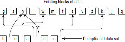
At the top of Figure 10.2 is an existing pool of stored data. Below this pool is a new data set that has been written to the system. This data set is deduplicated, as any block in the data set that already exists in our pool of existing data is stripped out of the new data set and replaced with a pointer.

When replacing multiple copies of the same data with a single copy plus a pointer for each additional copy, the magic is that pointers consume virtually no space, especially when compared to the data they are replacing. If each square in our example in Figure 10.2 is 16 KB in size, and each pointer is 1 KB, we have saved 90 KB. Each of the six pointers consumes only 1 KB, giving a total of 6 KB to store the pointers, instead of the 6 × 16 KB that would have been required to store the six blocks of data.

Deduplication is similar to but subtly different from compression. Deduplication identifies data patterns that have been seen before, but unlike compression, these patterns don't have to be close to each other in a file or data set. Deduplication works across files and directories and can even work across entire systems that are petabytes (PB) in size. A quick and simple example follows. In the manuscript for this chapter, the word storage has been used 204 times (this may change by the time the chapter goes to production). A simple deduplication algorithm could take one instance of the word storage and remove every other instance, replacing them with a pointer back to the original instance. For this example, let's assume that the word storage consumes 4 KB, while a pointer consumes only 1 KB. If we don't deduplicate, and we stick with the 204 instances of the word, we'll consume 816 KB (204 × 4 KB). But if we do deduplicate, the 204 references to the word will consume only 207 KB (4 KB for the initial copy, plus 204 × 1 KB for the other 203 pointers). Now let's assume that our deduplication worked across all chapters of the book (each chapter is a separate Microsoft Word document); we would save even more space! Obviously this is an oversimplified example, but it works for getting the concept across.

Deduplication is not too dissimilar to compression. It has been widely adopted for backup and archive use cases, and has historically seen slow uptake with primary storage systems based on spinning disk. However, many of the all-flash storage arrays now on the market implement data deduplication.

Block-Based Deduplication

Block-based deduplication aims to store only unique blocks in a system. And while the granularity at which the deduplication occurs varies, smaller granularities are usually better—at least from a capacity optimization perspective.

Two major categories of granularity are often referred to in relation to deduplication technologies:

• File level
• Block level

File-level granularity, sometimes referred to as single-instance storage (SIS), looks for exact duplicates at the file level and shouldn't really be called deduplication.

Block-level deduplication works at a far smaller granularity than whole files and is sometimes referred to as a subfile by the SNIA. And because it works at a much finer granularity than files, it can yield far greater deduplication ratios and efficiencies.

File-level deduplication (single instancing) is very much a poor-man's deduplication technology, and you should be aware of exactly what you are buying! On the other hand, block-level deduplication with block granularity of about 4 KB is generally thought of as being up there with the best.

Let's take a closer look at file single instancing and block-level deduplication.

File-Level Single Instancing

To be honest, file-level deduplication, also known as single instancing, is quite a crude form of deduplication. In order for two files to be considered duplicates, they must be exactly the same. For example, let's assume the Microsoft Word document for this chapter is 1.5 MB. If I save another copy of the file, but remove the period from the end of this sentence in that copy, the two files will no longer be exact duplicates, requiring both files to be independently saved to disk, consuming 3 MB. However, if the period were not removed, the files would be identical and could be entirely deduplicated, meaning only a single copy would be stored to disk, consuming only 1.5 MB.

That example isn't very drastic. But what happens when I create a PowerPoint file on Monday that is 10 MB and then on Tuesday I change a single slide and save it in a different folder? I will then have two files that will not deduplicate and that consume a total of about 20 MB, even though the two files are identical other than a minor change to one slide. Now assume I edit another slide in the same presentation on Wednesday and save it to yet another folder. Now I have three almost-identical files, but all stored separately and independently, consuming about 30 MB of storage. This can quickly get out of control and highlights the major weakness with file single instancing. It works, but it's crude and not very efficient.

Fixed-Length Block Deduplication

Deduplicating at the block level is a far better approach than deduplicating at the file level. Block-level deduplication is more granular than file-level deduplication, resulting in far better results.

The simplest form of block-level deduplication is fixed block, sometimes referred to as fixed-length segment. Fixed-block deduplication takes a predetermined block size—say, 16 KB—and chops up a stream of data into segments of that block size (16 KB in our example). It then inspects these 16 KB segments and checks whether it already has copies of them.

Let's put this into practice. We'll stick with a fixed block size of 16 KB, and use the 1.5 MB Word manuscript that I'm using to write this chapter. The 1.5 MB Word document gives us ninety-six 16 KB blocks. Now let's save two almost-identical copies of the manuscript. The only difference between the two copies is that I have removed the period from the end of this sentence in one of the copies. And to keep things simple, let's assume that this missing period occurred in the sixty-fifth 16 KB block. With fixed-block deduplication, the first sixty-four 16 KB blocks (1,024 KB) would be exactly the same in both files, and as such would be deduplicated. So we would need to store only one copy of each of the sixty-four 16 KB blocks—saving us 1 MB of storage. However, the thirty-two remaining 16 KB blocks would each be different, meaning that we cannot deduplicate them (replace them with pointers). The net result is that we could save the two almost-identical copies of the manuscript file, using up 2 MB of storage space instead of 3 MB. This is great, but it can be better.

Now then, the reason that all of the blocks following the omission of the period would be recognized as unique rather than duplicates is based on the nature of fixed-block deduplication. Quite often with fixed-block approaches to deduplication, as soon as you change one block in a data set, all subsequent blocks become offset and no longer deduplicate. This is the major drawback to fixed-block deduplication, as shown in Figure 10.3.

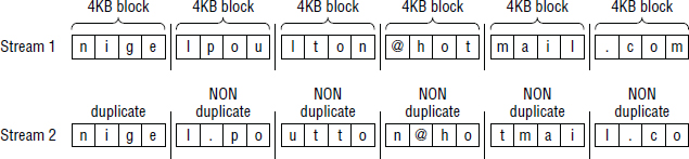
The example in Figure 10.3 shows two almost-identical email addresses. The only difference is the period in the local part of the email address in stream 2. As you can see, every block following the inclusion of the period is offset by one place, and none of the following blocks are identical, meaning none can be deduplicated.

Variable Block Size

Variable block, also known as variable length segment, approaches to deduplication pick up where fixed block started to struggle. Variable-block approaches apply a dynamic, floating boundary when segmenting a data set, reducing, even further, the impact of making changes to blocks. They also base their decisions about where each block begins and ends not by size alone but also by recognizing repeating patterns in the data itself. This means when there's an insertion, or removal, as in our period example, the variable-block method will realign with the existing data when it sees the repeating patterns. Most of the time, variable block size deduplication technologies will yield greater storage efficiencies than both fixed block and file single instancing.

Hashing and Fingerprinting

Let's take a look at the most common way of indexing and determining duplication of blocks.

Every block of data that is sent to and stored in a deduplicating system is given a digital fingerprint (unique hash value). These fingerprints are indexed and stored so they can be looked up very quickly. They're often stored in cache. If the index is lost, it can usually be re-created, although the process of re-creating can be long and keep the system out of service while it's being re-created.

When new writes come into a system that deduplicates data, these new writes are segmented, and each segment is then fingerprinted. The fingerprint is compared to the index of known fingerprints in the system. If a match is found, the system knows that the incoming data is a duplicate (or potential duplicate) block and replaces the incoming block with a much smaller pointer that points to the copy of the block already stored in the system.

Where to Deduplicate

Data can be deduplicated in various places. In typical backup use cases, deduplication is commonly done in one or more of the following three ways:

• Source
• Target
• Federated

Let's look at each option in turn.

Source-Based Deduplication

Source-based deduplication—sometimes referred to as client-side deduplication—requires agent software installed on the host and is where the heavy lifting work of deduplication is done on the host, consuming host resources including CPU and RAM. However, source-based deduplication can significantly reduce the amount of network bandwidth consumed between the source and target—store less, move less! This can be especially useful in backup scenarios where a large amount of data is being streamed across the network between source and target.

Because of its consumption of host-based resources and its limited pool of data to deduplicate against (it can only deduplicate against data that exists on the same host), it is often seen as a lightweight first-pass deduplication that is effective at reducing network bandwidth. Consequently, it is often combined with target-based deduplication for improved deduplication ratios.

Target-Based Deduplication

Target-based deduplication, sometimes referred to as hardware-based deduplication, has been popular for a long time in the backup world. In target-based deduplication, the process of deduplication occurs on the target machine, such as a deduplicating backup appliance. These appliances tend to be purpose-built appliances with their own CPU, RAM, and persistent storage (disk). This approach relieves the host (source) of the burden of deduplicating, but it does nothing to reduce network bandwidth consumption between source and target.

It is also common for deduplicating backup appliances to deduplicate or compress data being replicated between pairs of deduplicating backup appliances. There are a lot of deduplicating backup appliances on the market from a wide range of vendors.

Federated Deduplication

Federated deduplication is a distributed approach to the process of deduplicating data. It is effectively a combination of source and target based, giving you the best of both worlds—the best deduplication ratios as well as reduced network bandwidth between source and target.

This federated approach, whereby the source and target both perform deduplication, can improve performance by reducing network bandwidth between the source and target, as well as potentially improving the throughput capability of the target deduplication appliance. The latter is achieved by the data effectively being pre-deduplicated at the source before it reaches the target.

Technologies such as Symantec OpenStorage (OST) allow for tight integration between backup software and backup target devices, including deduplication at the source and target.

It is now common for many backup solutions to offer fully federated approaches to deduplication, where deduplication occurs at both the source and target.

When to Deduplicate

I've already mentioned that the process of deduplication can occur at the source, or target, or both. But with respect to target-based deduplication, the deduplication process can be either of the following:

• Inline
• Post-process

Let's take a look at both approaches.

Inline Deduplication

In inline deduplication, data is deduplicated in real time—as it is ingested, and before being committing to disk on the backend. Inline deduplication often deduplicates data while in cache. We sometimes refer to this as synchronous deduplication.

Inline deduplication requires that all hashes (fingerprinting) and potential bit-for-bit compare operations must occur before the data is committed to disk. Lightweight hashes are simpler and quicker to perform but require more bit-for-bit compares, whereas stronger hashes are more computationally intensive but require fewer bit-for-bit compare operations.

The major benefit to inline deduplication is that it requires only enough storage space to store deduplicated data. There is no need for a large landing pad where non-deduplicated data arrives and is stored until it is deduplicated at a later time.

The potential downside to inline deduplication is that it can have a negative impact on data-ingestion rates—the rate, in MBps, that a device can process incoming data. If a system is having to segment, fingerprint, and check for duplications for all data coming into the system, there is a good chance this may negatively impact performance.

Although inline deduplication works really well for small, medium, and large businesses, they can be particularly beneficial for small businesses and small sites for which the following are true:

• You want to keep your hardware footprint to a minimum, meaning you want to deploy as little storage hardware as possible.
• Your backup window—the time window during which you can perform your backups—is not an issue, meaning that you have plenty of time during which you can perform your backups.

In these situations, inline deduplication can be a good fit. First, you need to deploy only enough storage required to hold your deduplicated data. Also, because you are not having to squeeze your backup jobs into a small time window, the potential impact on backup throughput incurred by the inline deduplication process is not a concern.

Post-process Deduplication

Post-process deduplication is performed asynchronously. Basically, data is written to disk without being deduplicated, and then at a later point in time, a deduplication process is run against the data in order to deduplicate it.

In a post-process model, all hashes and bit-for-bit compare operations occur after the data has been ingested, meaning that the process of deduplicating data does not have a direct impact on the ability of the device to ingest data (MBps throughput). However, on the downside, this approach requires more storage, as you need enough storage capacity to house the data in its non-deduplicated form, while it waits to be deduplicated at a later time.

Most backup-related deduplication appliances perform inline deduplication, because most modern deduplication appliances have large amounts of CPU, RAM, and network bandwidth to be able to deal relatively well with inline deduplication.

Backup Use Case

Deduplication technologies are now a mainstay of just about all good backup solutions. They are a natural fit for the types of data and repeated patterns of data that most backup schedules comprise. During a single month, most people back up the same files and data time and time again. For example, if your home directory gets a full backup four times each month, that is at least four times each month that the same files will be backed up, and that's not considering any incremental backups that might occur between the four full backups mentioned. Sending data like this to a deduplication appliance will normally result in excellent deduplication.

Deduplicating backup-related data also enables longer retention of that data because you get more usable capacity out of your storage. You might have 100 TB of physical storage in your deduplication appliance, but if you are getting a deduplication ratio of 5:1, then you effectively have 500 TB of usable capacity. Also, as a general rule, the longer you keep data (backup retention), the better your deduplication ratio will be. This is because you will likely be backing up more and more of the same data, enabling you to get better and better deduplication ratios.

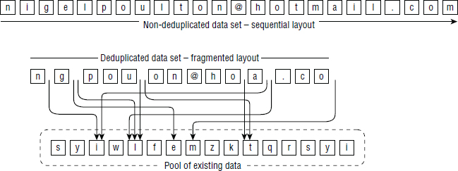
However, deduplication technologies tend to fragment file layouts. Duplicated data is referenced by pointers that point to other locations on the backend. Figure 10.4 shows the potential sequential layout of a data set before being deduplicated, as well as the same data set after deduplication. Although the deduplicated version of the filesystem consumes far less space, reading back the entire contents of the deduplicated data set will be a lot more difficult and take a lot more time than reading back the entire contents of the non-deduplicated data set. This is especially the case with spinning disk–based systems, though it is much less of an issue for solid-state systems.

The fragmenting of data layout has a direct impact on backup-related technologies such as synthetic full backups. A synthetic full backup is a full backup that is not created the normal way by sending all data from the source to the target. Instead, a synthetic full backup is created by taking a previous full backup that already exists on the target and applying any incremental backups that have occurred since that full backup, effectively creating a new full backup without having to read all data on the source and send it across the network to the target. Although synthetic full backups are popular these days, they are a challenge for deduplication systems. In order to create the synthetic full backup, a previous full backup has to be read from the deduplication appliance, plus any incremental backups taken since, and at the same time the deduplication appliance has to write out the new synthetic full backup. All of this reading and writing (which includes lots of heavy random reading because the deduplicated data is fragmented on the system) can severely impact the performance of the deduplication appliance.

Virtualization Use Case

Deduplication can lend itself well to virtualization technologies such as server and desktop virtualization. These environments tend to get good deduplication ratios thanks to the fact that x number of virtual Windows servers will share a very high percentage of the same core files and blocks. The same goes for other operating systems such as Linux.

For example, if you have a 10 TB image of a Windows server and deploy 100 servers from that image, those 100 servers will share a massive number of identical files and blocks. These will obviously deduplicate very well. Deduplication like this can also lead to potential performance improvements if you have a large read cache, because many of these shared files and blocks will be highly referenced (frequently read) by all virtual machines, causing them to remain in read cache where they can be accessed extremely quickly. If each of these 100 virtual servers had to access its own core files in individual locations on disk in our storage array, this would require our storage array to do a lot of work seeking and reading from the disks on the backend. This would result in poor performance. However, if these core files and blocks were deduplicated and only the master copies were frequently accessed, they could be accessed from cache memory at much faster speeds than if each read had to go to the backend disks.

Primary Storage and Cloud Use Cases

The rise of all-flash arrays has started pushing deduplication technologies to the forefront in primary storage use cases. Traditionally, deduplication has been avoided for primary storage systems because of the performance impact. However, that performance impact was mainly due to the nature of spinning disk and its poor random-read performance. After all, good random-read performance is vital for the following two deduplication-related operations:

• Performing bit-for-bit compare operations
• Performing read operations on deduplicated data

If bit-for-bit compare operations take a long time, they will impact the overall performance of the systems. Also, because the process of deduplicating data often causes it to be fragmented, reading deduplicated data tends to require a lot of random reading. All-flash arrays don't suffer from random-read performance problems, which makes deduplication technologies in primary storage very doable. In fact, most all-flash arrays support inline deduplication, and it's so tightly integrated to some all-flash arrays that they don't allow you to turn the feature off!

Tier 3 and cloud are also places where deduplication technologies are a good fit because accessing data from lower-tier storage, and especially from the cloud, is accepted to be slow. Adding the overhead of deduplication on top of this is not a major factor on the performance front, but it can be significant at reducing capacity utilization.

Deduplication Summary

Deduplication is similar in some ways to compression, but it is not the same. That said, deduplication and compression can be used in combination for improved space savings, though you will need to know the following:

• Deduplicated data can be compressed.
• Compressed data usually cannot be deduplicated.

If you want to use the two in combination, dedupe first, and compress second.

Some data types will deduplicate better than others; that's just life.

Deduplicating data tends to lead to random/fragmented data layout, which has a negative performance impact on spinning disk drives, but it is not a problem for flash and other solid-state media.

File-level deduplication is a poor-man's deduplication and does not yield good deduplication ratios. Variable-block deduplication technologies that can work at small block sizes tend to be the best.

Auto-Tiering

Sub-LUN auto-tiering is available in pretty much all disk-based storage arrays that deploy multiple tiers of spinning disk, and sometimes a smattering of flash storage. While it doesn't allow you to increase your usable capacity as deduplication and compression technologies do, it absolutely does allow you to optimize your use of storage resources.

Auto-tiering helps to ensure that data sits on the right tier of storage. The intent usually is for frequently accessed data to sit on fast media such as flash memory or 15K drives, and infrequently accessed data to sit on slower, cheaper media such as high-capacity SATA and NL-SAS drives or maybe even out in the cloud.

The end goal is to use your expensive, high-performance resources for your most active, and hopefully most important, data, while keeping your less frequently accessed data on slower, cheaper media.

Sub-LUN Auto-Tiering

Early implementations of auto-tiering worked at the volume level; tiering operations, such as moving up and down the tiers, acted on entire volumes. For example, if part of a volume was frequently accessed and warranted promotion to a higher tier of storage, the entire volume had to be moved up. This kind of approach could be extremely wasteful of expensive resources in the higher tiers if, for example, a volume was 200 GB and only 2 GB of it was frequently accessed and needed moving to tier, 1 but auto-tiering caused the entire 200 GB to be moved.

This is where sub-LUN auto-tiering technology came to the rescue. Sub-LUN tiering does away with the need to move entire volumes up and down through the tiers. It works by slicing and dicing volumes into multiple smaller extents. Then, when only part of a volume needs to move up or down a tier, only the extents associated with those areas of the volume need to move. Let's assume our 200 GB volume is broken into multiple extents, each of which is 42 MB (as implemented on most high-end Hitachi arrays). This time, if our 200 GB volume had 2 GB of hot data (frequently accessed) that would benefit from being moved to tier 1, the array would move only the 42 MB extents that were hot, and wouldn't have to also move the cold (infrequently accessed) 42 MB extents. That is a far better solution!

Obviously, a smaller extent size tends to be more efficient than a larger extent size, at least in the context of efficiently utilizing capacity in each of our tiers. Some mid-range arrays have large extent sizes, in the range of 1 GB. Moving such 1GB extents is better than having to move an entire volume, but if all you need to move up or down the tiers is 10 MB of a volume, it could still be improved on. In this case, an even smaller extent size, such as 42 MB or even smaller, should clearly be more efficient. Smaller extent sizes also require less system resources to move around the tiers. For example, moving 1 GB of data up or down a tier takes a lot more time and resources than moving a handful of 42 MB extents. However, small extent sizes have a trade-off too. They require more system resources, such as memory, to keep track of them.

Tiers of Storage

In the world of tiering, three seems to be the magic number. The vast majority of tiered storage configurations (maybe with the exception of purpose-built hybrid arrays) are built with three tiers of storage.

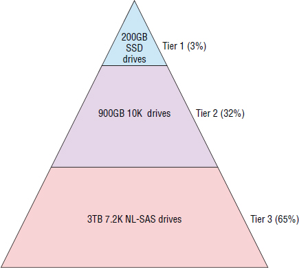
Exactly what type of storage you put in each tier depends, but a common approach is for tier 1 to be solid-state storage (flash memory), tier 2 to be fast spinning disk such as 10K or 15K SAS drives, and tier 3 to be big, slow SATA or NL-SAS drives. However, how much of each tier you have and similar concerns are highly dependent upon your environment and your workload. If possible, you should work closely with your vendors and technology partners to determine what is right for your environment.

A common three-tiered design used in the real world is shown in Figure 10.5. The percentage values represent how much of the overall system capacity is in each tier. They do not refer to the percentage of overall disk drives each tier has.

Activity Monitoring

To make tiering-related decisions such as which extents to move up the tiers and which to move down the tiers, a storage array needs to monitor activity on the array. This monitoring usually involves keeping track of which extents on the backend are accessed the most and which are accessed the least. However, the times of day when you monitor this activity can be crucial to getting the desired tiering results. For example, many organizations choose to monitor data only during core business hours, when the array is servicing line-of-business applications. By doing this, you are ensuring that the extents that move up to the highest tiers are the extents that your key line-of-business applications use. In contrast, if you monitor the system outside business hours (say, when your backups are running), you may end up with a situation where the array moves the extents relating to backup operations to the highest tiers. In most situations, you won't want backup-related volumes and extents occupying the expensive high-performance tiers of storage, while your line-of-business applications have to make do with cheaper, lower-performance tiers of storage.

Arrays and systems that let you fine-tune monitoring periods are better than those that give you less control. The more you understand about your environment and the business that it supports, the better you will be able to tune factors such as the monitoring period, and the better the results of your tiering operations will be.

Tiering Schedules

Similar to fine-tuning and custom-scheduling monitoring windows, the same can be done for scheduling times when data can move between tiers. As with creating custom monitoring periods, defining periods when data can move between tiers should be customized to your business. After all, moving data up and down tiers consumes system resources, resources that you probably don't want consumed by tiering operations in the middle of the business day when your applications need those resources to service customer sales and the perform similar functions.

A common approach to scheduling tiering operations (moving data up and down through the tiers) is to have them occur outside business hours—for example, from 3 a.m. to 5 a.m.—when most of your systems are quiet or are being backed up.

Configuring Tiering Policies

As well as customizing monitoring and movement windows, it will often be useful to configure policies around tiering. Some common and powerful polices include the following:

• Exclusions
• Limits
• Priorities

Exclusions allow to you do things such as exclude certain volumes from all tiering operations, effectively pinning those volumes into a single tier. They also allow you to do things such as exclude certain volumes from occupying space in certain tiers. For example, you may not want volumes relating to backups to be able to occupy the highest tiers.

Limits allow you limit how much of a certain tier a particular volume or set of volumes can occupy.

Priorities allow you to prioritize certain volumes over others when there is contention for a particular tier. As an example, your key sale app might be contending with a research app for tier 1 flash storage. In this situation, you could assign a higher priority to volumes relating to your sales app, giving those volumes preference over other volumes and increasing the chances that the volumes associated with the sales app will get the space on tier 1.

Of course, not all arrays and systems support all features. Do your research before assuming your choice of technology can do all of the preceding tasks.

Array Size Concerns

Unfortunately, auto-tiering solutions don't suit every scenario. One scenario where they may not be the best choice is smaller arrays and smaller storage systems. A major reason for that is the number of spindles (drives) each tier of storage has. For example, a small storage array with 32 drives installed might be well suited to a single tier of storage configured into a single pool, meaning that all volumes have access to all 32 spindles. If you try to divide such a small system into three tiers of storage (for example, four flash drives, twelve 15K drives, and sixteen SATA drives), you may find that each tier has too few spindles to make any tier performant enough, and the benefits of the flash storage may be outweighed by the backend operations required to move data up and down the tiers. Also, auto-tiering is sometimes a licensed feature, adding cost to an array. Often this additional cost isn't beneficial on small arrays.

As a general rule, instead of utilizing auto-tiering on smaller arrays, you may be better off having a single tier of medium- to high-performance drives such as 10K SAS drives, maybe supplemented with a flash cache, where flash drives are utilized as a second level of cache rather than a persistent tier of storage.

Remote Replication

An often unconsidered side-effect of auto-tiering is the potential imbalance between source and target arrays that are replicated. For example, in a replicated configuration where one array is considered the primary array (has live hosts attached to it) and the other array considered the secondary array (has standby hosts attached to it), the primary array sees all of the read and write workload. As a result of this read and write workload, the auto-tiering algorithms of the array move extents up and down the tiers, ensuring an optimal layout. However, the target array does not see the same workload. All the target array sees is replicated I/O, and only write I/Os are replicated from the source to the target. Read I/Os are not replicated. As a result, how a volume is spread across the tiers on the target array will often be very different from how it's spread across the tiers on the source array. This frequently results in a volume being on lower-performance tiers on the target array. This can be a problem if you ever have to bring systems and applications up on the target array, because they may perform lower than they did on the source array. This is just one more thing to consider with auto-tiering.

Summary

In this chapter we covered all of the prevalent capacity optimization technologies in the modern storage world. We started out by talking about Thin Provisioning and the difference between thick and thin volumes, from both a capacity and performance perspective. We then talked about how thin provisioning enables overprovisioning, and the potential cost savings this can bring. We finished off our discussion on thin provisioning by talking about zero space reclamation technology and how this is maturing and helping us keep thin volumes thin. We then talked about inline and post-process compression deduplication, being careful to point out the differences and use cases for each, as well as what to watch out for when using the two technologies side-by-side. We finished the chapter talking about auto-tiering and how it enables us to more efficiently use our capacity by placing the right data on the right tiers of storage.

Chapter Essentials

Thin Provisioning Thin provisioning (TP) technologies allow you to loan out more storage than you physically have, resulting in higher utilization of storage resources. This is known as overprovisioning and must be managed and monitored so you do not overrun the physical capacity in your storage array.

Compression Compression technologies re-encode data so it can be stored and transmitted using fewer bits and bytes, enabling you to store more data with less physical capacity, as well as transmit data quicker over networks consuming less bandwidth. Compression technologies are part of all good backup solutions and are increasingly popular in all-flash storage arrays.

Deduplication Deduplication technologies allow you to squeeze more usable capacity out of your storage systems. Deduplication works by recognizing duplicate blocks of data, and replacing the duplicate blocks with pointers. Variable-block deduplication is recognized as a leading approach to deduplication. Deduplication technologies are part of all good backup solutions and are increasingly popular in all-flash storage arrays.

Sub-LUN Auto-Tiering While sub-LUN auto-tiering technologies do not increase your usable capacity, they do allow you to more efficiently utilize your storage resources. Sub-LUN auto-tiering works by placing frequently accessed blocks of data on high-performance media such as solid-state media, while placing infrequently accessed blocks of data on slower, cheaper storage media. Smaller extent sizes yield better efficiencies with sub-LUN auto-tiering technologies.