User resource limits

There are a number of resources that databases utilize at much higher numbers than typical servers. These include file descriptors, semaphores, and user processes.

I/O scheduler

Input/Output (I/O) scheduling is the method that operating systems use to decide the order in which block level I/O operations will be submitted to storage volumes. By default, these schedulers often assume they are working with spinning disks that have high seek latency. Thus, the default is usually an elevator algorithm that attempts to order requests by location and to minimize seek times. In Linux, you might see the following options available:

wtf@host:~$ cat /sys/block/sda/queue/scheduler
[noop] anticipatory deadline cfq

The noop scheduler is the proper choice when the target block device is an array of SSDs with a controller that performs I/O optimization. Every I/O request is treated equally because seek times on solid-state drives (SSDs) are relatively stable. The deadline scheduler will optimize by seeking to minimize I/O latency by imposing deadlines to prevent starvation and by prioritizing reads over writes. The Deadline Scheduler has shown to be more performant in highly concurrent multithreaded environments, such as database loads.

Memory allocation and fragmentation

No one can deny that databases are some of the most memory-hungry applications a server can run. Understanding how memory is allocated and managed is critical to utilizing it as effectively as possible. Database binaries are compiled using a variety of memory allocation libraries. Here are some examples:

• MySQL’s InnoDB, as of version 5.5, uses a custom library that wraps glibc’s malloc. GitHub claims to have saved 30% latency by switching to tcmalloc, whereas Facebook uses jemalloc.

• PostgreSQL also uses its own custom allocation library, with malloc behind it. Unlike most other datastores, PostgreSQL allocates memory in very large chunks, called memory contexts.

• As of version 2.1, Apache Cassandra off-heap allocation supports jemalloc over native.

• MongoDB’s version 3.2 implementation uses malloc by default but can be configured with tcmalloc or jemalloc.

• As of version 2.4, Redis uses jemalloc.

jemalloc and tcmalloc have both proven to provide significant improvements in concurrency for most database workloads, performing significantly better than glibc’s native malloc while also reducing fragmentation.

Memory is allocated in pages that are 4 KB in size by default. Thus, 1 GB of memory is the equivalent of 262,144 pages. CPUs use a page table that contains a list of these pages, with each page referenced through a page table entry. A translation lookaside buffer (TLB) is a memory cache that stores recent translations of virtual memory to physical addresses for faster retrieval. A TLB miss is where the virtual-to-physical page translation is not in a TLB. A TLB miss is slower than a hit, and can require a page walk, requiring several loads. With large amounts of memory, and thus pages, TLB misses can create thrashing.

Transparent Huge Pages (THP) is a Linux memory management system that reduces the overhead of TLB lookups on machines with large amounts of memory by using larger memory pages, thus reducing the number of entries required. THPs are blocks of memory that come in 2 MB and 1 GB sizes. Tables used for 2 MB pages are suitable for gigabytes of memory, whereas 1 GB pages are best for terabytes. However, defragmentation of these large page sizes can cause significant CPU thrashing, which has been seen on Hadoop, Cassandra, Oracle, and MySQL workloads, among others. To mitigate this, you might need to deal with disabling defragmentation and losing up to 10% of your memory because of it.

Linux is not particularly optimized for database loads requiring low latency and high concurrency. The kernel is not predictable when it goes into reclaim mode, and one of the best recommendations we can give is to simply ensure that you never fully use your physical memory by reserving it to avoid stalls and significant latency impacts. You can reserve this memory by not allocating it in configuration.

Swapping

In Linux/UNIX systems, swapping is the process of storing and retrieving data that no longer fits in memory and needs to be saved to disk to alleviate pressure for memory resources. This is a very slow operation by orders of magnitude compared to memory access, and thus should be considered a last resort.

It is generally accepted that databases should avoid swapping because it can immediately increase latency beyond acceptable levels. That being said, if swap is disabled, the operating system “Out of Memory Killer” (OOM Killer) will shut down the database process.

There are two schools of thought here. The first, and more traditional, approach is that keeping a database up and slow is better than the database not being available at all. The second approach, and the one that aligns more closely with the DBRE philosophy, is that latency impacts are as bad as performance impacts; thus, swapping in from disk should not be tolerated at all.

Database configurations will typically have a realistic memory usage high watermark as well as a theoretical one. Fixed memory structures like buffer pools and caches will consume fixed amounts, making them predictable. At the connection layer, however, things can get messier. There is a theoretical limit based on the maximum number of connections and the maximum size of all per-connection memory structures, such as sort buffers and thread stacks. Using connection pools and some sane assumptions, you should be able to predict a reasonably safe memory threshold by which you can avoid swapping.

This process does allow for anomalies such as misconfigurations, runaway processes, and other pear-shaped events to push you past your memory bounds, which would shut down your server in an OOM event. This is a good thing, though! If you have effective visibility, capacity, and failover strategies in place, you have effectively shut out a potential Service-Level Objective (SLO) violation on latency.

Should you choose to allow swapping in your environment, you can reduce the operating system’s chance of swapping out your database memory for file cache, which is generally not helpful. You can also adjust the OOM scores for your database processes to reduce the chance that your kernel memory profiler will kill your database process for memory needs elsewhere.

Non-Uniform memory access

Early implementations of multiple processors used an architecture called Symmetric Multiprocessing (SMP) to provide equal access to memory for each CPU via a shared bus between the CPUs and the memory banks. Modern multiprocessor systems utilize Non-Uniform Memory Access or NUMA, which provides a local bank of memory to each processor. Access to memory banked to other processors is still done over a shared bus. Thus, some memory access has much lower latency (local) versus others (remote).

In a Linux system, a processor and its cores are considered a node. The operating system attaches memory banks to their local nodes and calculates cost between nodes based on distance. A process and its threads will be given a preferred node to utilize for memory. Schedulers can change this temporarily, but affinity will always go to the preferred node. On top of this, after memory is allocated, it will not be moved to another node.

What this means in an environment in which large memory structures are present, such as database buffer pools, is that memory will be allocated heavily to the preferred node. This imbalance will cause the preferred node to be filled, with no available memory on it. This means that even if you are utilizing less memory than physically available on the server, you will still see swapping.

At this point, for most DBMS requests, you set interleaving for NUMA in the kernel. Stories abound for PostgreSQL, Redis, Cassandra, MongoDB, MySQL, and ElasticSearch about the same issues.

Network

The assumption of this book is that all datastores are distributed. Network traffic is critical for the performance and availability of your databases, period. You can break up network traffic into the following categories:

• Internode communications

• Application traffic

• Administrative traffic

• Backup and recovery traffic

Internode communications include data replication, consensus and gossip protocols, and cluster management. This is the data that let’s the cluster know its own state and keeps data replicated in the amounts defined. Application traffic is the traffic that comes from application servers or proxies. This is what maintains application state and allows for the creation, mutation and deletion of data by applications.

Administrative traffic is the communication between management systems, operators, and the clusters. Administrative traffic is the communication between management systems, operators, and clusters. This includes starting and stopping services, deploying binaries, and making database and configuration changes. When things go badly elsewhere, this is the lifeline to systems that allows for manual and automated recovery. Backup and recovery traffic is just what it says. This is the traffic created when archiving and copying data, moving data between systems or recovering from backups.

Isolation of traffic is one of the first steps to proper networking for your databases. You can do this via physical network interface cards (NICs), or by partitioning one NIC. Modern server NICs generally come in 1 Gbps and 10 Gbps sizes, and you can bond them in a pair to allow for redundancy and load balancing. Although this redundancy will increase mean time between failures (MTBF), it is an example of creating robustness rather than resiliency.

Databases need a lean transport layer to manage their workloads. Frequent and fast connections, short round trips, and latency-sensitive queries all require a specific tuning effort. This can be broken down into three areas:

• Tuning for large numbers of connections by expanding the amount of TCP/IP ports.

• Reducing the time it takes to recycle sockets to avoid large amounts of connections sitting in TIME_WAIT, and thus rendering it unusable.

• Maintaining a large TCP backlog so that saturation will not cause connections to be refused.

TCP/IP will become your best friend in troubleshooting latency and availability problems. We strongly suggest that you deep-dive into this. A good book to do so is Internetworking with TCP/IP, Vol 1 by Douglas E. Comer (Pearson). It is updated as of 2014 and is an excellent reference.

Storage

Storage for databases is a huge topic. You need to consider the individual disks, the grouped configuration of disks, controllers providing access to disks, volume management software, and the filesystems on top of this. It is quite possible to geek out on any single section of this for days, so we will try to stay focused on the big picture here.

In Figure 5-1, you can see the ways in which data is propagated to storage. When you read from a file, you go from user buffer, to page cache, to disk controller, to disk platter for retrieval, and then step back through that for delivery to the user.

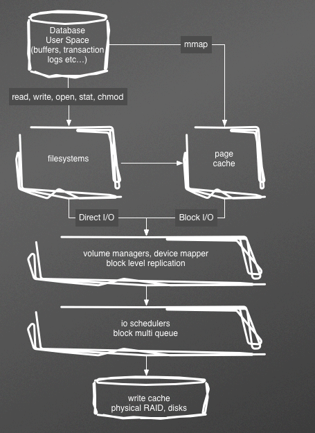
Figure 5-1. The linux storage stack

This elaborate cascade of buffers, schedulers, queues, and caches is used to mitigate the fact that disks are very slow compared to memory, with the difference being 100 nanoseconds versus 10 milliseconds.

For database storage, you will have five major demands, or objectives:

• capacity

• throughput (or IO per second, aka IOPS)

• latency

• availability

• durability

Storage capacity

Capacity is the amount of space available for the data and logs in your database. Storage can be via large disks, multiple disks striped together (RAID 0), or multiple disks functioning as individual mount points (known as JBOD, or just a bunch of disks). Each of these solutions has a different failure pattern. Single large disks are single points of failure, unless mirrored (RAID 1). RAID 0 will have its MTBF reduced by a factor of N, where N is the number of disks striped together. JBOD will have more frequent failures, but unlike RAID 0, the other N–1 disks will be available. Some databases can take advantage of this and stay functional, if degraded, while the replacement disk is acquired and installed.

Understanding a database’s total storage needs is only one piece of this picture though. If you have a 10 TB storage need, you can create a 10 TB stripe set, or mount ten 1 TB disks in JBOD and distribute data files across them. However, you now have a 10 TB database to back up at once, and if you have a failure, you will need to recover 10 TB, which takes a long time. During that time, you will have reduced capacity and availability for your overall system. Meanwhile, you must consider if your database software, the operating system, and the hardware can manage the concurrent workloads to read and write to this monolithic datastore. Breaking this system up into smaller databases will improve resiliency, capacity, and performance for applications, for backup/restores, and for copying the dataset.

Storage throughput

IOPS is the standard measure of input and output operations per second on a storage device. This includes reads and writes. When considering the needs, you must consider IOPS for the peak of a database’s workload rather than the average. When planning a new system, you will need to estimate the number of IOPS needed per transaction, and the peak transactions in order to plan appropriately. This will obviously vary tremendously depending on the application. An application that does constant inserts and single row reads can be expected to do four or five IOPs per transaction. Complex multiquery transactions can do 20 to 30 easily.

Database workloads tend to be mixed read/write, and random, rather than sequential. There are some exceptions, such as append-only write schemas (such as Cassandra’s SSTables), which will write sequentially. For hard disk drives (HDDs), random IOPs numbers are primarily dependent upon the storage device’s random seek time. For SSDs, random IOPs numbers are instead constrained by internal controller and memory interface speeds. This explains the significant improvement in IOPS seen by SSDs. Sequential IOPS indicate the maximum sustained bandwidth that the disk can produce. Often sequential IOPS are reported as megabytes per second (MBps), and are indicative of how a bulk load or sequential writes might perform.

When looking at SSDs, remember to consider the bus, as well. Consider installing a PCIe bus flash solution, such as FusionIO 6 GBps throughput with microsecond latency. As of this writing, 10 TB will cost you around $45,000, however.

Traditionally, IOPS was the constraining factor over storage capacity. This is particularly true for writes, which you could not optimize away via caching like reads. Adding disks via striping (RAID 0) or JBOD would add more IOPS capacity just like storage. RAID 0 will give you uniform latency and eliminate hot spots that might show up in JBOD, but at the expense of a reduced MTBF based on the number of disks in the stripe set.

Storage latency

Latency is the end-to-end client time of an I/O operation; in other words, the time elapsed between sending an I/O to storage and receiving an acknowledgement that the I/O read or write is complete. As with most resources, there are queues for pending requests, which can back up during saturation. Some level of queuing is not a bad thing, and, in fact, many controllers are designed to optimize queue depth. If your workload is not delivering enough I/O requests to fully use the performance available, your storage might not deliver the expected throughput.

Transactional database applications are sensitive to increased I/O latency and are good candidates for SSDs. You can maintain high IOPS while keeping latency down by maintaining a low queue length and a high number of IOPS available to the volume. Consistently driving more IOPS to a volume than it has available can cause increased I/O latency.

Throughput-intensive applications like large MapReduce queries are less sensitive to increased I/O latency and are well-suited for HDD volumes. You can maintain high throughput to HDD-backed volumes by maintaining a high queue length when performing large, sequential I/O.

The Linux page cache is another bottleneck to latency. By using direct IO (O_DIRECT), you can avoid multimillisecond latency impacts by bypassing the page cache.

Storage availability

Performance and capacity are critical factors, but unreliable storage must be accounted for. Google did an extensive study on HDD failure rates in 2007 titled "Failure Trends in a Large Disk Drive Population" (see Figure 5-2). From this, you can expect about 3 out of 100 drives to fail in their first three months of service. Of disks that make it through the first six months, you will find approximately 1 in 50 fail between six months and one year in service. This doesn’t seem like a lot, but if you have six database servers with eight drives each, you can expect to have a disk failure during that period.

Figure 5-2. HDD failure rates, according to Google

This is why engineers began mirroring drives, à la RAID 1, and enhancing stripe sets with a parity drive. We don’t talk much about the parity variants (e.g., RAID 5) because their write penalty is so large. Modern storage subsystems will typically find disks in JBOD or grouped in stripes (RAID 0), mirrors (RAID 1), or mirrors that are striped (RAID10). With that in mind, it is easy to extrapolate that RAID 1 and RAID 10 are most tolerant of single-disk failures, whereas RAID 0 is most prone to complete service loss (and greater chances the more disks in the stripe). JBOD shows the ability to tolerate failures while still serving the rest of the storage.

Availability is not just the MTBF of your volumes. It is also the time it would take to rebuild after a failure, or the mean time to recover (MTTR). The choice of RAID 10 versus RAID 0 is dependent on the ability to easily deploy replacement database hosts during a failure. It can be tempting to stay with RAID 0 for performance reasons. RAID 1 or 10 requires double the IOPS for writes, and if you are using high-end drives, the duplication of hardware can become expensive. RAID 0 is performant and predictable, but somewhat fragile. After all, a five-drive stripe set of HDDs can be expected to have about a 10% failure rate in the first year. With four hosts, you can reasonably expect a failure every year or two.

With a mirror, you can replace the disk without the need to rebuild the database. If you are running a 2 TB database with fairly fast-spinning disks, database backup copy time is measured in hours, and you will likely need more hours for database replication to sync the delta from the last backup. To be comfortable with this, you will need to consider if you have enough capacity to support peak traffic with one, or even two, failed nodes while this recovery is going on. In a sharded environment, where one dataset is only a percentage of users, this might be perfectly acceptable, meriting more fragile data volumes for the benefits of cost and/or write latency.

Durability

Finally, there is durability. When your database goes to commit data to physical disk with guarantees of durability, it issues an operating system call known as fsync() rather than relying on page cache flushing. An example of this is when a redo log or write-ahead log is being generated and must be truly written to disk to ensure recoverability of the database. To maintain write performance, many disks and controllers utilize an in-memory cache. fsync instructs the storage subsystem that these caches must be flushed to disk. If your write cache is backed by a battery, and can survive a power loss, it is much more performant to not flush this cache. It is important to validate that your particular setup does truly flush data to stable storage, whether that is a non-volatile RAM (NVRAM), write cache or the disk platters themselves. You can do this via a utility such as diskchecker.pl by Brad Fitzpatrick.

Filesystem operations can also cause corruption and inconsistency during failure events, such as crashes. Journaling filesystems like XFS and EXT4 significantly reduce the possibility of such events, however.