Chapter 10. Data Storage, Indexing, and Replication
We’ve been talking about operations for much of this book in preparation for diving into datastores. The most critical thing every datastore has in common with one another is that they...wait for it...store data. In this chapter, we explain the ways a single node structures its data storage, how large datasets are partitioned, and how nodes replicate data between one another. It’s going to be quite the chapter!
This book’s scope is focused predominantly on reliability and operations, so we will be working on understanding storage and access patterns to facilitate infrastructure choices, to understand performance characteristics, and to make sure that you, as the database reliability engineer (DBRE), have the information required to help engineering teams choose the appropriate datastores for their services. For a much more detailed and nuanced review of this, we strongly suggest that you read Martin Kleppmann’s book Designing Data-Intensive Applications (O’Reilly).
Data Structure Storage
Databases traditionally have stored data in a combination of tables and indexes. A table is the main storage mechanism, and an index is an optimized subset of data ordered to improve access times. With the proliferation of datastores now, this has evolved significantly. Understanding how data is written to and read from storage is crucial to being able to configure and optimize your storage subsystems and databases.
When understanding how a database stores data, you actually need to evaluate not only how the raw data is stored, but also how it is retrieved. In large datasets, accessing specific subsets of data at any reasonable level of latency will often require specialized storage structures, called indexes, to accelerate the finding and retrieval of that data. Thus, when looking at storage, we must take into account the storage and Input/Output (I/O) requirements for putting data onto disk and into indexes as well as the I/O requirements for retrieving that data.
Database Row Storage
Much of the data here is applicable to more traditional relational systems. We will begin with this, and then we’ll discuss some of the more prevalent alternative storage options. In relational databases, data is stored in containers called blocks or pages that correspond to a specific number of bytes on disk. Different databases will use blocks or pages in their terminology. In this book, we use blocks to refer to both. Blocks are the finest level of granularity for storing records. Oracle Database stores data in data blocks. A page is a fixed size called a block, just like blocks on disks. Blocks are the smallest size that can be read or written to access data. This means that if a row is 1 K and the block size is 16 K, you will still incur a 16 K read operation. If a database block size is smaller than the filesystem block size, you will be wasting I/O for operations that require multiple pages. This can be visualized in Figure 10-1.

Figure 10-1. Aligned versus nonaligned block/stripe configurations.
A block requires some metadata to be stored, as well, usually in the form of a header and trailer or footer. This will include disk address information, information about the object the block belongs to, and information about the rows and activity that have occurred within that block. In Oracle, as of version 11g, Release 2, block overhead totals 84 to 107 bytes. In MySQL’s InnoDB, as of version 5.7, header and trailer use 46 bytes. Additionally, each row of data will require its own metadata, including information about columns, links to other blocks that the row is spread across, and a unique identifier for the row.1
Data blocks are often organized into a larger container called an extent. For efficiency reasons, an extent is often the allocation unit when new blocks are required within a tablespace. A tablespace is typically the largest data structure, mapped to one or more physical files that can be laid out as required on disk. On systems mapped directly to physical disks, tablespace files can be laid out across different disks to reduce I/O contention. In the paradigms we focus on in this book, such curation of I/O is not necessarily an option. Large, generic RAID structures of stripes and potentially mirrored stripes can maximize I/O without significant time spent on microtuning. Otherwise, assuming rapid recovery and failover are available, focusing on simple volumes or even ephemeral storage provides ease of management and minimal overhead.
B-tree structures
Most databases structure their data in a binary tree format, also known as B-tree. A B-tree is a data structure that self-balances while keeping data sorted. The B-tree is optimized for the reading and writing of blocks of data, which is why B-trees are commonly found in databases and filesystems.
You can imagine a B-tree table or index as an upside-down tree. There is a root page, which is the start of the index that is built on a key. The key is one or more columns. Most relational database tables are stored on a primary key, which can be explicitly or implicitly defined. For instance, a primary key can be an integer. If an application is looking for data that maps to a specific ID or a range of IDs, this key will be used to find it. In addition to the primary key B-tree, secondary indexes on other columns or sets of columns can be defined. Unlike the original B-tree, these indexes store only the data that is indexed rather than the entire row. This means that these indexes are much smaller and can fit in memory much more easily.
A B-tree is called a tree because when you navigate through the tree, you can choose from two or more child pages to get to the data you want. As just discussed, a page contains rows of data and metadata. This metadata includes pointers to the pages below it, also known as child pages. The root page has two or more pages below it, also known as children. A child page, or node, can be an internal node or a leaf node. Internal nodes store pivot keys and child pointers and are used to direct reads through the index to one node or another. Leaf nodes contain key data. This structure creates a self-balancing tree that can be searched within only a few levels, which allows for only a few disk seeks to find the pointers to the rows that are needed. If the data needed is within the key itself, you don’t even need to follow the pointer to the row.
Binary tree writes
When inserting data to a B-tree, the correct leaf node is found via search. Nodes are created with room for additional inserts, rather than packing them in. If the node has room, the data is inserted in order in the node. If the node is full, a split has to occur. In a split, a new median is determined and a new node is created. Records are then redistributed accordingly. The data about this median is then inserted into the parent node, which can cause additional splits all the way up to the root node. Updates and deletes also begin with finding the correct leaf node via search, followed by the update or delete. Updates can cause splits if they increase data size to the point where it overflows a node. Deletes can cause rebalancing, as well.
Greenfield (new) databases begin with primarily sequential writes and reads. This shows as low latency writes and reads. As the database grows, splits will cause I/O to become random. This results in longer latency reads and writes. This is why we must insist on realistic datasets during testing to ensure that long-term performance characteristics will exhibit rather than these naive, early exhibitors.
Single-row writes require a page to be completely rewritten, at minimum. If there are splits, there can be many pages that must be written. This complex operation requires atomicity yet allows opportunities for corruption and orphaned pages if there is a crash. When evaluating a datastore, it is vital to understand what mechanisms are put in place to prevent this. Examples of such mechanisms include the following:
Logs of write operations that are written to before the more complex operations of writing to disk, also known as Write Ahead Logs (WAL)
Event logs for reconstruction
Redo logs with before and after images of the mutated data
With all of this in mind, a crucial variable in configuring your databases for underlying storage is the database block size. We’ve discussed the importance of aligning database block sizes with the underlying disk block sizes, but that is not enough. If you are using Solid-State Drives (SSDs), for instance, you might find smaller block sizes provide much better performance while traversing B-trees. An SSD can experience a 30% to 40% latency penalty on larger blocks versus performance on Hard Disk Drives (HDDs). Because reads and writes are required in B-tree structures, this must be taken into account.
The following is a summary of the attributes and benefits of B-trees:
Excellent performance for range-based queries.
Not the most ideal model for single-row lookups.
Keys exist in sorted order for efficient key lookups and range scans.
Structure minimizes page reads for large datasets.
By not packing keys into each page, deletes and inserts are efficient, with only occasional splits and merges being needed.
Perform much better if the entire structure can fit within memory.
When indexing data, there are other options as well. The most predominant one is the hash index.
As we mentioned earlier, the B-tree tends to be fairly ubiquitous in relational databases. If you’ve worked in those environments, you’ve probably worked with them already. There are other options for data storage, however, and they are moving from experimental to mature. Let’s look next at append-only log structures.
Sorted-String Tables and Log-Structured Merge Trees
BigTable, Cassandra, RocksDB (which is available in MySQL via MyRocks and MongoDB), and LevelDB are all examples of databases that use sorted-string tables (SSTs) for primary storage. The terms SSTable and Memtable originally appeared in the Google BigTable paper that has been a source of inspiration for a number of database management systems (DBMS’s) since then.
In an SST storage engine, there are a number of files, each with a set of sorted key–value pairs inside. Unlike in the block storage discussed earlier, there is no need for the metadata overhead at the block or row level. Keys and their values are opaque to the DBMS and stored as arbitrary binary large objects (BLOBs). Because they are stored in a sorted fashion, they can be read sequentially and treated as an index on the key by which they are sorted.
There is an algorithm that combines in-memory tables, batch flushing, and periodic compaction in SST storage engines. This algorithm is referred to a log-structured merge (LSM) tree architecture (see Figure 10-2). This was described by Patrick O’Neill in his paper.
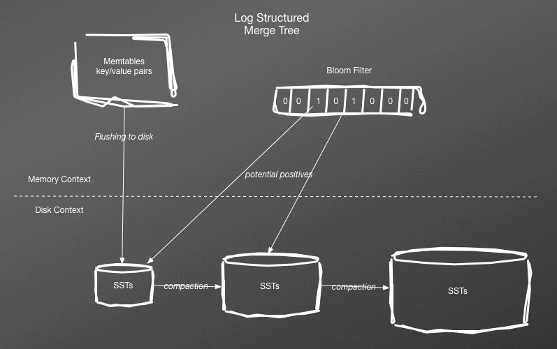
Figure 10-2. Log-structured merge tree structure with a bloom filter
With an LSM, SSTs are written to by periodic flushes of data that has been stored in memory. After data is flushed, sorted, and written to disk, it is immutable. Items cannot be added or removed from the map of key–value pairs. This is effective for read-only datasets because you can map an SST into memory for rapid access. Even if the SST does not fully fit in memory, random reads require a minimal amount of disk seeks.
To support fast writes, more is required. Opposite to writes on disk, writes on a dataset in memory are trivial because you are just changing pointers. An in-memory table can take writes and remain balanced. This is also referred to as a memtable. The memtable can also act as the first query point for reads before falling back to the newest SST on disk, followed by the next oldest, and then the next, until the data is found. After a certain threshold is reached, which can be time, number of transactions, or size, the memtable will be sorted and flushed to disk.
When deletes are done on data that is already stored in an SST, a logical delete must be recorded. This is also known as a tombstone. Periodically, SST’s are merged together, allowing elimination of tombstones and saving of space. This merge and compaction process can be very I/O intensive and often requires significantly more space available than the actual working set. Until operations teams are used to these new capacity models, there might be impacts to availability Service-Level Objectives (SLOs).
There are data-loss possibilities that must be assumed during failure scenarios. Until memtables are flushed to disk, they are vulnerable to crashes. Unsurprisingly, there are similar solutions in SST storage engines as in B-tree based ones, including event logs, redo logs, and write ahead logs.
Bloom filters
You might imagine that having to search through a memtable and a large number of SSTables to find a record key that doesn’t exist could be expensive and slow. You’d be right! An implementation detail to assist with this is a bloom filter. A bloom filter is a data structure that you can use to evaluate whether a record key is present in a given set, which, in this case, is an SSTable.
A datastore such as Cassandra uses bloom filters to evaluate which SSTable, if any, might contain the record key requested. It is designed for speed, and thus there might be some false positives. But, the overall effect is a significant reduction in read I/O. Inversely, if a bloom filter says that a record key does not exist in an SSTable, that is a certainty. Bloom filters are updated when memtables are flushed to disk. The more memory that can be allocated to the filter, the less likely a false positive will occur.
Implementations
There a number of datastores that utilize the LSM structure with SSTables as a storage engine:
Apache Cassandra
Google Bigtable
HBase
LevelDB
Lucene
Riak
RocksDB
WiredTiger
Implementation details will vary for each datastore, but the proliferation and growing maturity of this storage engine has put it into an important storage implementation for any team working with large datasets to understand.
While reviewing and enumerating data storage structures, we’ve mentioned logs multiple times as critical for data durability in the case of failures. We also discuss them in (Chapter 7). They are also critical for replicating data in distributed datastores. Let’s dig deeper into logs and their usage in replication.
Indexing
We have already discussed one of the most ubiquitous of indexing structures, the B-tree. SSTs are also inherently indexed. There are some other index structures that you will find out in the database wild.
Hash indexes
One of the simplest index implementations is that of a hash map. A hash map is a collection of buckets that contain the results of a hash function applied to a key. That hash points to the location where the records can be found. A hash map is only viable for single-key lookups because a range scan would be prohibitively expensive. Additionally, the hash must fit in memory to ensure performance. With these caveats, hash maps provide excellent access for the specific use cases for which it works.
Bitmap indexes
A bitmap index stores its data as bit arrays (bitmaps). When you traverse the index, it is done by performing bitwise logical operations on the bitmaps. In B-trees, the index performs the best on values that are not repeated often. This is also known as high cardinality. The bitmap index functions much better when there are a small number of values being indexed.
Permutations of B-trees
There are permutations of the traditional B-tree index. These are often designed for very specific use cases, including the following:
- Function Based
An index based on the results of a function applied to the index.
- Reverse Index
Indexing values from the end of that value to the beginning to allow for reverse sorting.
- Clustered Index
Requires the table records to be physically stored in indexed order to optimize I/O access. The leaf nodes of clustered index contain the data pages.
- Spatial Index
There are a number of different mechanisms for indexing spatial data. Standard index types cannot handle spatial queries efficiently.
- Search Index
These indexes allow for searching of subsets of data within the columns. Most indexes cannot search within the indexed value. There are some indexes designed for this, however, and some entire datastores, such as ElasticSearch, are built for this operation.
Each datastore will have its own series of specialized indices that are available, often to optimize the typical use cases within that datastore.
Indexes are tremendously critical for rapid access of subsets of data. When evaluating bleeding-edge datastores, understanding the limitations in terms of indexes, such as the ability to have more than one index or how many columns can be indexed or even how those indexes are maintained in the background, is crucial to understand.
Logs and Databases
Logs began as a way to maintain durability in database systems. They evolved to the mechanism used to replicate data from primary to replica servers for availability and scalability reasons. Eventually, services were built to use these logs to migrate data between different database engines with a transformation layer between them. This then evolved into a full messaging system with logs becoming events that a subscribing service could use to perform discreet pieces of work for downstream services.
With opportunities of so many use cases for logs, we’d like to focus specifically on replication in this chapter. Having discussed how data can be stored and indexed on a local server, we now will move on to how that data can be distributed to other servers.
Data Replication
For this entire book, we have been working under the assumption that you will be working primarily on distributed datastores. This means that there must be a way for data that is written on one node to be moved around between nodes. There are entire books written on this topic alone,2 so we will focus on well-known and utilized examples rather than more theoretical ones. Our goal for you as a DBRE is for you and the engineers you support to be able to look at replication methods offered and to understand how they work. Knowing the pros and cons and patterns and antipatterns that are associated with replication options is crucial for a DBRE, an architect, a software engineer, or an operations person to do their jobs well.
There are some high-level distinctions in replication architectures that can be used for an initial enumeration. When discussing replication here, we are referring to leaders as nodes that take writes from applications and followers as nodes that receive replicated events to apply to their own datasets. Finally, readers are nodes that applications read data from.
- Single Leader
Data is always sent to one specific leader.
- Multiple Leader
There can be multiple nodes with a leader role, and each leader must persist data across the cluster.
- No Leader
All nodes are expected to be able to take writes.
We will begin with the simplest replication method, single-leader, and build on from there.
Single-Leader
As the title implies, in this replication model all writes go to a single leader and are replicated from there. Thus, you have one node out of N nodes that is designated as the leader, and the others are replicas. Data flows from the leader out. This method is widely utilized for its simplicity, and you can make a few guarantees. These guarantees include:
There will be no consistency conflicts because all writes occur against one node.
Assuming that all operations are deterministic, you can guarantee that they will result in the same outputs on each node.
There are some permutations here, such as one leader replicating to a few relay replicas that then have their own replicas. Regardless, there is one leader taking writes, which is the key attribute of this architecture. There are a few different approaches to replication in single leader. Each approach trades off some level of consistency, latency, and availability. Thus, the appropriate choice will vary based on the applications and how they use database clusters.
Replication models
When replicating data in single-leader fashion, there are three different models that you can be use:
- Asynchronous
optimize latency over durability
- Synchronous
optimize durability over latency
- Semi-synchronous
compromise latency and durability
In asynchronous replication models, a transaction is written to a log on the leader and then committed and flushed to disk. A separate process is responsible for shipping those logs to the followers, where they are applied as soon as possible. In asynchronous replication models, there is always some lag between what is committed on the leader and what is committed on the followers. Additionally, there is no guarantee that the commit point on one follower is the same as the others. In practice, the time gap between commit points might be too small to notice. It is just as easy to find clusters using asynchronous replication for which there is a time gap of seconds, minutes, or hours between leaders and followers.
In synchronous replication models, a transaction that is written to a log on the leader is shipped immediately over the network to the followers. The leader will not commit the transaction until the followers have confirmed that they have recorded the write. This ensures that every node in the cluster is at the same commit point. This means that reads will be consistent regardless of what node they come from, and any node can take over as a leader without risk of data loss if the current leader fails. On the other hand, network latency or degraded nodes can all cause write latency for the transaction on the leader.
Because synchronous replication can have a significant impact on latency, particularly if there are many nodes, semi-synchronous replication can be put in place as a compromise. In this algorithm, only one node is required to confirm to the leader that they have recorded the write. This reduces the risk of latency impacts when one or more nodes are functioning in degraded states while guaranteeing that at least two nodes on the cluster are at the same commit point. In this mode, there is no longer a guarantee that all nodes in the cluster will return the same data if a read is issued on any reader. There is, however, still a guarantee that you can promote at least one node in the cluster to leader status, if needed, without data loss.
Replication log formats
To achieve single-leader replication, you must use a log of transactions. There are a number of approaches to how these logs are implemented. Each one has benefits and trade-offs, and many datastores might implement more than one to allow you to choose what works best. Let’s review them here.
Statement-based logs
In statement-based replication, the actual SQL or data write statement used to execute the write is recorded and shipped from the leader to followers. This means that the entire statement will be executed on each follower.
Pros:
A statement can execute hundreds or thousands of records. That’s a lot of data to ship. The statement is usually much smaller. This can be optimal when replicating across datacenters where network bandwidth is scarce.
This approach is very portable. Most SQL statements will result in the same outputs even on different versions of the database. This allows you to upgrade followers before upgrading leaders. This is a critical piece of high-availability approaches to upgrades in production. Without backward-compatible replication, version upgrades can require significant downtime while an entire cluster is upgraded.
You can also use log files as audits and for data integration because they contain entire statements.
Cons:
A statement might require significant processing time if it is using aggregation and calculation functions on a selected dataset to determine what it will write. Running the statement can take much longer than simply changing the records or bits on disk. This can cause replication delay in serialized apply processes.
Some statements might not be deterministic and can create different outputs to the dataset if run on different nodes.
Write-ahead logs
A write-ahead log (WAL), also known as a redo log, contains a series of events, each event mapped to a transaction or write. In the log are all of the bytes required to apply a transaction to disk. In systems, such as PostgreSQL, that use this method, the same log is shipped directly to the followers for application to disk.
Pros:
Very fast as the parsing and execution of the statement has already occurred. All that is left is to apply the changes to disk.
Not at risk of impacts from nondeterministic SQL.
Cons:
Can consume significant bandwidth in high-write environments.
Not very portable because the format is closely tied to the database storage engine. This can make it challenging to perform rolling upgrades that allow for minimization of downtime.
Not very auditable.
WALs will often use the same logs built for durability and just bolt on a log shipping process for replication. This is what gives us the efficiency of this format, but also its lack of portability and flexibility.
Row-based replication
In row-based replication (also called logical), writes are written to replication logs on the leader as events indicating how individual table rows are changed. Columns with new data are indicated, columns with updated information show before/after images, and deletes of rows are indicated as well. Replicas use this data to directly modify the row rather than needing to execute the original statement.
Pros:
Not at risk of impacts from nondeterministic SQL.
A compromise on speed between the two previous algorithms. Logical translation to physical is still required, but entire statements do not need to run.
A compromise on portability between the two pervious algorithms. Not very human readable but can be used for integrations and inspection.
Cons:
Can consume significant bandwidth in high-write environments.
Not very auditable.
This method has also been called change data capture (CDC). It exists in SQL Server and MySQL and is also used in data warehouse environments.
Block-level replication
So far, we have been speaking about replication methods using native database mechanisms. In contrast, block-device replication is an external approach to the problem. A predominant implementation of this is Distributed Replicated Block Device (DRBD) for Linux. DRBD functions a layer above block devices and propagates writes not only to the local block device, but also to the replicated block device on another node.
Block-level replication is synchronous and eliminates significant overhead in the replicated write. However, you cannot have a running database instance on the secondary node. So, when a failover occurs, a database instance must be started. If the former master failed without a clean database shutdown, this instance will need to perform recovery just as if the instance had been restarted on the same node.
So, what we have with block-level replication is synchronous replication with very low latencies, but we lose the ability to use the replicas for scalability or workload distribution. Happily for us, using an external replication method, such as block-level replication, can be combined with native replication, such as statement-based or row-level replication. This can give a combination of zero-data-loss replication along with the flexibility of asynchronous replication.
Other methods
There are other methods for replication that are decoupled from the database logs. Extraction, Transform, and Load (ETL) jobs used to move data between services will often look for indicators of new or changed rows such as IDs or timestamps. With these indicators, they will pull out data for loading elsewhere.
Triggers that are on tables can also load a table with changes for an external process to listen on. These triggers can simply list out IDs for changes or give full change data capture information just like a row-based replication approach will.
When evaluating options for replication, you will need a combination of options depending on your source datastore, target datastore, and the infrastructure that exists between the two datastores. We will discuss this more in the next section on replication uses.
Single-leader replication uses
At this point in datastore maturity, replication is more often than not a requirement rather than an option. But, there are still a variety of reasons to implement replication that can affect architecture and configuration. In single-leader architectures, most of these can be enumerated as availability, scalability, locality, and portability.
Availability
It goes without saying that if a database leader fails, you want to have the fastest recovery option possible to which to point application traffic. Having a live database with a fully up-to-date copy of data is far preferable to a backup that must be recovered and then rolled forward to the failure point. This means that mean time to recover (MTTR) requirements and data-loss requirements must be kept at the forefront when making choices about replication. Synchronous and semi-synchronous replication gives the best options for no data loss with a low MTTR, but they do affect latency. Finding the elusive trifecta of low MTTR, low latency, and no data loss via replication alone is not possible without some external support, such as a messaging system that you can write to in addition to the datastore to allow for recovery of data that might be lost in a leader failover in an asynchronously replicated environment.
Scalability
A single leader creates a boundary on write I/O, but the followers allow for reads of data to scale based on the number of reads provided. For read-intensive applications that experience a relatively small amount of writes, multiple replicas do create an opportunity for creating more capacity in the cluster. This capacity is bounded, as replication overhead does not allow for linear scalability. Still, this does create an opportunity for increasing runway. To support scalability, the data on replicas must be recent enough to support business requirements. For some organizations, the replication delay inherent in asynchronously replicated systems is acceptable. However, for other requirements, synchronous replication is absolutely required, regardless of the impact to write latency.
Locality
Replication is also a way to keep datasets in various locations that are closer to consumers to minimize latency. If you have customers across countries or even on different coasts, the impact of long-distance queries can be significant. Large datasets are not very portable in their entirety, but incremental application of changes keeps those datasets up to date. As we mentioned previously, long-distance replication over bandwidth-starved networks often requires statement-based replication if compression is not enough to manage row-based or WAL entries. Modern networks and compression often alleviate this. Also, semi-synchronous or synchronous algorithms are generally not feasible with long-distance latencies, leading to the choice of asynchronous replication.
Portability
There are a number of opportunities in other datastores for the data residing in your leader. You can use replication logs to push into data warehouses as events for consumers in a data pipeline or for transformation into other datastores with more appropriate query and indexing patterns. Utilizing the same replication streams as replicas that are in place for availability and scale ensures that the datasets streaming from the leader are the same. That being said, more custom solutions such as query-based ETL and trigger-based approaches provide filtering of the appropriate subsets of data rather than the entire transaction stream coming out of the replication logs. These jobs also often have significant leeway in the freshness requirements of data, which allows for choices that have less of an impact on latency than other approaches.
Based on these needs, you and your engineering teams should be able to select one or more choices for replication. Regardless of which choices you make, there are a number of challenges that can come up in these replicated environments.
Single leader replication challenges
There a number of opportunities for challenges in any replicated environment. Even though single-leader is the simplest of replicated environments, that does not by any means indicate simplicity or ease. In this section, we walk through the most common of these challenges.
Building replicas
With large datasets, the portability of your data can be reduced significantly. We reviewed this in (Chapter 7). As the dataset increases, the MTTR also increases, which can lead to a need for a larger number of replicas or a new backup strategy that can keep the MTTR within acceptable levels. Other options include reducing the dataset size in one group of server by breaking out one dataset into multiple smaller datasets. This is also called sharding. We discuss this further in Chapter 12.
Keeping replicas synchronized
Building a replica is only the first step in a replicated environment. While using asynchronous replication, keeping that replica caught up proves to be its own challenge in environments characterized by frequent or large changes to the dataset. As we discussed in “Replication log formats”, changes must be logged, logs must be shipped, and changes must be applied.
Relational databases, by design, typically translate writes to a linearized series of transactions that must be followed strictly to ensure dataset consistency between replicas and leaders. This generally translates into the need for serialized processes applying one change at a time on the replicas. These serialized apply processes on replicas often are unable to catch up or stay caught up with the leader for a number of reasons, including the following:
Lack of concurrency and parallelism as compared to the leader. I/O resources are often wasted on the replicas.
Blocks to be read in transactions are not in memory on replicas if read traffic is not common.
When distributing writes to leaders and reads to replicas, read traffic concurrency can affect write latency on replicas.
Regardless of the reason, the end result is often called replica lag. In some environments, replica lag might be an infrequent and ephemeral problem that resolves itself frequently, and within SLOs. In other environments, these issues become pervasive and can lead to replicas being unusable for their original purposes. If this occurs, there is an indication that the workload for your datastore has grown too large and must be redistributed via one or more techniques. We discuss these techniques in more detail in Chapter 12. In brief, they are as follows:
- Short Term
Increase capacity on the cluster so that the current workload fits within the clusters capacity.
- Medium Term
Break out functions of the database into their own clusters to guaranty workload bounds fit within the cluster capacity. Also known as functional partitioning or sharding.
- Long Term
Break out your dataset into multiple clusters, allowing you to maintain workload bounds so that they fit within the cluster’s capacity. Also known as dataset partitioning or sharding.
- Long Term
Choose a database management system whose storage, consistency, and durability requirements make more sense for your workload and SLOs and that will not have the same scaling problems.
As you can see in the choices described, none of these will work for continued growth. In other words, they do not scale linearly with workload. Some, like capacity increases of functional partitioning, have shorter runways than others, like dataset partitioning. But even dataset partitioning will eventually find limits in how far it can be solved. This means that other things must be evaluated to ensure that the bounds never increase to the point of diminishing returns that render the solution obsolete.
If you are experiencing replication lag and must mitigate impacts while a longer-term solution is put in place, there are some short-term tactics that can be employed. These include:
Preloading active replica datasets into memory to reduce disk IO.
Relaxing durability on the replicas to reduce write latency.
Parallelizing replication based on schemas if there are no transactions that cross schemas.
These are all short term tactics that can allow for breathing room, but they all also have tradeoffs in terms of fragility, high maintenance costs, and potential data issues so they must be scrutinized very carefully and only in great need.
Single leader failovers
One of the greatest values of replication is the existence of other datasets that are caught up and can be used as leaders in the case of a failure or because of the need to move traffic off of the original leader. This is not a trivial operation, however, and there are a number of steps that occur. In a planned failover, these steps include the following:
Identification of the replica that you want to promote to the new leader.
Depending on the topology, a preliminary partial reconfiguration of the cluster can be performed, to move all replicas to replicate from the candidate leader.
If asynchronous replication is used, a pause in application traffic to allow the candidate leader to catch up.
Reconfiguration of all application clients to point to the new replica.
In a clean, planned failover, this all can appear to be quite trivial if you’ve effectively scripted and automated certain steps. However, relying on these failovers during failure scenarios can create lots of opportunity for problems. An unplanned failover might look something like this:
Leader database instance becomes unresponsive.
A monitoring heartbeat process attempts to connect to the database leader.
After 30 seconds of hanging, the heartbeat triggers a failover algorithm.
The failover algorithm does the following:
Identifies the replica with the latest commit level as the promotion candidate
Reattaches the other replicas at the appropriate point in the log stream to the promotion candidate
Monitors until the cluster replicas are caught up
Reconfigures application configurations via file or a service and pushes
Instantiates rebuilding of a new replica
Within this, there are numerous inflection points. We discuss these further in Chapter 12.
Despite these challenges, replication remains one of the most commonly implemented features of databases and thus becomes a critical part of the database infrastructure. This means that it must be incorporated into the rest of your reliability infrastructure.
Single leader replication monitoring
Effective management of replication requires effective monitoring and operational visibility. There are a number of metrics that must be collected and presented to ensure that replicas are effective in supporting the organization’s SLOs. Critical areas to monitor include the following:
Replication lag
Latency impacts to writes
Replica availability
Replication consistency
Operational processes
This is touched upon somewhat in Chapter 4, but is worth mentioning again here.
Replication lag and latency
To understand replication flows, we must understand the relative time it takes to perform replicated operations. In asynchronous environments, this means understanding the amount of time that has lapsed between an operation occurring on the master and the time when that write has been applied to the replica. This time can vary wildly from second to second, but the data is crucial. There are a number of ways that you can measure this.
Like any distributed system, these measurements rely at some level on the local machine time. Should system clocks or Network Time Protocol (NTP) drift apart from one another, the information can be skewed. There is simply no way to rely on local time on two machines and assume that they are synchronized. For most distributed databases relying on asynchronous replication, this is not an issue. Times are very close, and this will suffice. But, even in these situations, remembering the fact that time is a very relative concept on each node can assist in forensics on some troubling issues.
One common approach to measuring the time from insert on a leader to insert on a replica is to insert a heartbeat row of data and then to measure when that time appears on the replica. For example, if you insert data at 12:00:00 and you regularly poll the replica and see that it has not received that value, you can assume that replication is stalled. If you query at 12:01:00 and the data for 11:59:00 does exist, but 12:00:00 and beyond doesn’t, you know replication is one second behind at 12:01:00. Eventually, this row will commit, and you can use the next row to measure how far beyond the database is currently.
In the case of semi- or fully synchronous replication, you will want to know the impact of these configurations on writes. This can and will be measured as part of your overall latency metrics, but you will also want to measure the time the network hops from the leader to the replica takes because this will be the cost of synchronous writes over the network.
The following are critical metrics that you must ensure are being gathered:
Delay in time from leader to replica in asynchronous replication
Network latency between leader and replicas
Write latency impact in synchronous replication
These metrics are invaluable for any service. Proxy infrastructures can use replication lag information to validate which database replicas are caught up enough to take production read traffic. A proxy layer that can take nodes out of service not only assists in guaranteeing that stale reads do not occur, but also allows replicas that are behind to catch up without the burden of supporting read traffic. Of course this algorithm must take into account what happens if all replicas are delayed. Do you serve from the leader? Do you shed load at the frontend until enough replicas are caught up? Do you put the system in read-only mode? All of these are potentially effective options if planned for.
Additionally, engineers can use replica lag and latency information to troubleshoot data consistency issues, performance degradations, and other complaints that can result from replication delays.
Now, let’s look at the next set of metrics: on availability and capacity.
Replication availability and capacity
If you are working with a datastore such as Cassandra that distributes data synchronously based on a replication factor, you also need to monitor and be aware of the number of copies that are available to satisfy a quorum read. For instance, suppose that we have a cluster with a replication factor of 3, which means that a write must be replicated to three nodes. Our application requires that 2/3 of the nodes with this data must be able to return results during a query. This means that if we have two failures, we will no longer be able to satisfy our applications queries. Monitoring replica availability proactively lets you know when you are in danger of failing this.
Similarly, even in environments without replication factor and quorum requirements, database clusters are still designed with an eye toward how many nodes must be available in order to satisfy SLOs. Monitoring how cluster size matches these expectations is critical.
Finally, it is important to recognize when replication has broken completely. Although monitoring replication lag with heartbeats will inform you that replication is falling behind, it will not alert you that something has occurred and the replication stream is broken. There are a number of reasons that replication might break:
Network partitions
Inability to execute Data Manipulation Language (DML) in statement-based replication, including:
Schema mismatch
Nondeterministic SQL causing dataset drift that violates a constraint
Writes that went accidentally to the replica causing dataset drift
Permissions/security changes
Storage space starvation on replica
Corruption on replica
The following are examples of metrics to gather:
Actual number of available copies of data versus expected number
Replication breakage requiring repair of replicas
Network metrics between the leaders and replicas
Change logs for the database schemas and user/permissions
Metrics on how much storage is being consumed by replication logs
Database logs that provide more information about issues such as replication errors and corruption
With this information, automation can use replica availability metrics to deploy new replicas when you are underprovisioned. Operators can also more quickly identify the root cause of breakage to determine if they should repair or simply replace a replica or if there is a more systemic issue that must be addressed.
Replication consistency
As we discussed earlier, there are possible scenarios that can occur that will cause your datasets to be inconsistent between leader and replica. Sometimes, if this causes a replication event to fail during the apply phase, you will be alerted to this via replication breaking. What is even worse though, is silent corruption of data that you do not detect for quite a long time.
You will recall from Chapter 7 that we discussed the importance of a validation pipeline for maintaining consistency of datasets with business rules and constraints. You can utilize a similar pipeline to ensure that data is identical across replicas. Like data validation pipelines for consistency, this is often neither simple nor inexpensive in terms of resources. This means that you must be selective in determining which data objects are reviewed and how often.
Data that is append-only, such as SSTs or even insert-only tables in B-tree structures, is easier to manage because you can create checksums on a set of rows based on a primary key or date range and compare these checksums across replicas. As long as you let this run frequently enough that you don’t fall behind, you can be relatively sure that this data is consistent.
For data that allows for mutations, this can prove more challenging. One approach is to run and store a database-level hashing function on the data after a transaction is completed in the application. When incorporated into the replication stream, a hash will create identical values in each replica if the data replicated appropriately. If it didn’t, the hashes will be different. An asynchronous job that compares hashes on recent transactions can then alert if there is a difference.
These are just a few ways to monitor replication consistency. Creating patterns for your software engineers (SWEs) to use, as well as a classification system of data objects to help them determine if a table requires a place in a validation pipeline, will help to ensure that you don’t use too many precious resources. Sampling or just doing recent time windows may also be effective depending on the type of data that you are storing.3
Operational processes
Finally, it is important to monitor the time and resources required to perform operational processes critical to replication. Over time, as datasets and concurrency grow, these processes can grow more burdensome on a number of dimensions. If you exceed certain thresholds, you might be at risk of being able to maintain replication freshness or to keep an appropriate number of replicas online at any time to support traffic. Some of these metrics include:
Dataset size
Backup duration
Replica recovery duration
Network throughput used during backup and recovery
Time to synchronize after recovery
Impact to production nodes during backups
By sending events with appropriate metrics every time a backup, recovery, or synchronization occurs, you can create reports to evaluate and potentially predict when your dataset and concurrency will cause your operational processes to become unusable. You can also utilize some basic predictive evaluations on how durations or consumption of resources can change based on changes in dataset size or concurrency.
Outside of predictive automation, regular reviews and tests can help operations staff to evaluate when their operational processes are no longer scaling. This will allow you to either provision more capacity, to redesign systems or processes, or to rebalance dataset distributions to maintain effective times that support availability and latency SLOs.
Although there will inevitably be other metrics or indicators that you want to measure with respect to your data replication, these are a good working set to ensure that your replication is working effectively and is supporting the SLOs against which you designed it.
Single-leader replication is by far the most common implementation of replication due to its relative simplicity. Still, there are times when availability and locality needs are not met by this approach. By allowing writes into a database cluster from more than one leader, the effects of leader failovers can be reduced, and leaders can be put in different zones and regions to allow for better performance. Let’s now review the approaches and challenges of this requirement.
Multi-Leader Replication
There are really two different approaches to breaking free from the single-leader paradigm of replication. The first method is what we can call multi-directional replication, or traditional multileader. In this approach, the concept of a leader role still exists, and leaders are designed to take and propagate writes to replicas as well as to the other leader. Typically, there will be two leaders distributed into different datacenters. The second approach is write-anywhere, meaning that any node in the database cluster can effectively take reads or writes at any time. Writes are then propagated to all other nodes.
Regardless of which solution is attempted here, the end result is more complex because you must add a layer of conflict resolution. When all writes are going to one leader you are working with a premise that there can be no chance of conflicting writes going to different nodes. But, if you allow writes to multiple nodes, there is a chance that conflicts can occur. This must be planned for appropriately, causing increased application complexity.
Multileader use cases
If the end result of multileader replication is complexity, what requirements could be worth that cost and risk? Let’s look at them here.
Availability
When a leader failover occurs in single-leader asynchronous replication, there is generally an impact to the application of anywhere between 30 seconds on the low end and 30 minutes or even one or more hours on the high end, depending on how the system is designed. This is due to the need for replication consistency checks, crash recovery, or any of a number of other steps.
In some cases, this disruption to service might simply be unacceptable, and there are not resources or ability to change the application to tolerate the failovers more transparently. In this case, the ability to load balance writes across nodes becomes potentially worth the inevitable complications.
Locality
A business might need to run active sites in two different regions to ensure low latency for a global or distributed customer base. In a read-heavy application, you can still often do this via single-leader replication over a long-distance network. However, if the application is write intensive, the latency impact of sending writes across those long-distance networks might be too great. If this is the case, putting a leader in each datacenter and managing conflict resolution can prove to be the best approach.
Disaster recovery
Similar to locality and availability, there are times when an application is so critical that it must be separated across datacenters to ensure availability in the infrequent case of a failure at the datacenter layer. You can still accomplish this goal with single-leader replication but only if the secondary region is used for reads only, as discussed earlier, or if it is used only for redundancy. Few businesses can afford to spin up an entire datacenter without using it, however, so multileader replication is often chosen to allow both datacenters to actively take traffic and support customers.
With a greater percentage of infrastructures running in cloud services, or with global distribution requirements, it is almost an inevitability that you will need to evaluate multileader replication eventually for one of the aforementioned reasons. Often, the physical implementation of the multileader replication can be supported natively or with a third party piece of software. The challenge comes in managing the inevitable conflicts that will occur.
Conflict resolution in traditional multidirectional replication
Traditional multidirectional replication bears the closest resemblance to single leader. Essentially, it just pushes the writes both directions as you allow writes to go to more than one leader. It sounds good and meets all of the use cases we just discussed. But if you are using asynchronous replication, which is the only feasible approach in an environment incorporating multiple datacenters and slow network connections, there can and will be problems. During times of replication latency or partitioned networks, applications that rely on the stored state in the database will be using stale state. On repair of the replication lag or the network partition, the writes that have been built using different versions of state must be resolved. So how do you and your SWEs manage the problem of conflicting writes in a multileader replication architecture? Very carefully. As with most problems, we can work on this with a few approaches.
Eliminate conflicts
The path of least resistance is always avoidance. There are times when you can perform writes or direct traffic in such a way that there simply are no conflicts. Here are a few examples:
Give each leader a subset of primary keys that can be generated only on that specific leader. This works well for insert/append-only applications. At its simplest, this might look like one leader writing odd number incrementing keys and the other leader writing even number ones.
Affinity approaches in which a specific customer is always routed to a specific leader. You can do this by region, unique ID, or any number of ways.
Use a secondary leader for failover purposes only, effectively writing to only one leader at a time but maintaining a multileader topology for ease of use.
Shard at the application layer, putting full application stacks in each region to eliminate the need for active/active cross region replication.
Of course, just because you configure things this way doesn’t mean it will always work. Configuration mistakes, load balancer mistakes, and human errors are all possible and can cause replication to break or data to be corrupted. Thus, you still need to be prepared for accidental conflicts even if they are rare. And as we’ve discussed before, the rarer the error, the more dangerous it can be.
Last write wins
For the case in which you will not be able to avoid potential write conflicts, you need to decide how you want to manage them when they occur. One of the more common algorithms provided natively in datastores is Last Write Wins (LWW). In LWW, when two writes conflict, the write with the latest timestamp wins. This seems pretty straightforward, but there are a number of issues with timestamps.
Timestamps—Sweet Little Lies
Most server clocks use wall clock time, which relies on gettimeofday(). This data is provided by hardware and NTP. Time can flow backward instead of forward for many reasons, such as the following:
Hardware issues
Virtualization issues
NTP not being enabled, or upstream servers might be wrong
Leap seconds
Leap seconds are rather horrifying. POSIX days are defined as 86,400 seconds in length. Real days are not always 86,400 seconds, however. Leap seconds are scheduled to keep days in line, by skipping or double-counting seconds. This can cause tremendous problems, and Google spreads out the time over a day to keep time monotomic.
There are times when LWW is relatively safe. If you can perform immutable writes because you know the correct state of your data at the time of write, using LWW can work. But, if you are relying on state you’ve read in the transaction to perform a write, you are at significant risk of data loss in the case of a network partition.
Cassandra and Riak are examples of datastores with LWW implementations. In fact, in the Dynamo paper, LWW is one of the two options described for handling update conflicts.
Custom resolution options
Due to the constraints of basic algorithms that rely on timestamps, more custom options must often be taken into account. Many replicators will allow for custom code to be executed when a conflict is detected after a write. The logic required to automatically resolve write conflicts can be quite extensive, and even so, there can be opportunities for making mistakes.
Using optimistic replication, which allows for all mutations to be written and replicated, you can allow background processes, the application, or even users to determine what to do to resolve those conflicts. This can be as simple as choosing one version or another of the data object. Alternatively, you could do a full merge of the data.
Conflict-free replicated datatypes
Due to the complexity of logic in custom code for conflict resolution, many organizations might balk at the work and the risks. There is a class of data structures, however, that are built to effectively manage writes from multiple replicas that might have timestamp or network issues. These are called conflict free, replicated datatypes (CRDTs). CRDTs provide strong, eventual consistency as they are always able to be merged or resolved without conflicts. CRDTs are effectively implemented in Riak as of this writing and utilized in very large implementations of online chat and online betting.
As we can see here, conflict resolution in multi-leader environments is absolutely possible but not a simple problem. The complexity involved in distributed systems is very real and requires a significant amount of engineering time and effort. Additionally, mature implementations of these approaches might not be available in the datastores at which you and your organization work most effectively. So, be very careful before going down the rabbit hole of multileader replication.
Write-anywhere replication
There is an alternate paradigm to the traditional multidirectional replication. In a write-anywhere approach, there are no leaders. Any node can take reads or writes. Dynamo-based systems, such as Riak, Cassandra, and Voldemort are examples of this approach to replication. There are certain attributes of these systems that we will go over in more detail now:
Eventual consistency
Read and write quorums
Sloppy quorums
Anti entropy
Different systems will vary on their implementations of these, but together they form an approach to leaderless replication as long as your application can tolerate unordered writes. There are usually tunables that help modify the behavior of these systems to better match your needs, but the presence of unordered writes is an inevitability.
Eventual consistency
The phrase “eventual consistency,” is often touted in relation to a class of datastores known as NoSQL. In distributed systems, server or network issues will fail. These systems are distributed to allow for continued availability but at a cost in data consistency. With a node down for minutes, hours, or even days, nodes easily diverge in terms of the data stored within them4
When systems come back up, they will resolve using the methods discussed in the previous section on conflict resolution, including the following:
LWW via timestamps or vector clocks5
Custom code
Conflict free replicated datatypes
Although there is no guarantee that data is consistent across all nodes at any time, that data will eventually converge. When you build the datastores, you configure how many copies of the data must be written to provide quorum during failures.
That being said, eventual consistency still must be proven to work. There are plenty of opportunities for data loss, whether through misunderstanding of the conflict resolution techniques used and the results of their application or through bugs. Jepsen is a great test suite that shows how to effectively test data integrity in a distributed datastore. You can find some additional reading at the following:
Jepsen’s Distributed Systems Safety Research
Martin Fowler’s “Eventual Consistency”
Peter Bailis and Ali Ghodsi’s “Eventual Consistency Today: Limitations, Extensions, and Beyond”
Read and write quorums
One key factor in write anywhere replication is an understanding of how many nodes must be available to deliver or accept data to maintain consistency. At the client or database levels, there is generally an ability to define quorum. Historically, a quorum is the minimum number of members of a assembly necessary to conduct the business of that group. In the case of distributed systems, this means the minimum number of readers or writers necessary to guarantee consistency of data.
For instance, in a cluster of three nodes, you might want to tolerate one node’s failure. This means you require a quorum of two for reads and writes. When making decisions about quorums, there is an easy formula. N is the number of nodes in a cluster. R is the number of read nodes available, and W is the number of write nodes. If R + W is greater than N, you have an effective quorum to guarantee at least one good read after a write.
In our example of three nodes, this means that you need at least two readers and two writers given that 2 + 2 > 3. If you lose two nodes, you have only 1 + 1, or 2. That is less than 3, and thus you don’t have quorum, and the cluster should not return data on read. If on reading two nodes, the application receives two different results (either missing data on one node or divergent data), repair will be done using the defined conflict resolution methods. This is called a read repair.
There is a lot more to understanding quorums and all of the theory and practice of distributed systems. For more reading, we recommend the following:
Quorum Systems: With Applications to Storage and Consensus
Sloppy quorums
There will be times when you have nodes up, but they do not have the data needed to meet quorum. Perhaps N1, N2, and N3 are configured to take writes, and N2 and N3 are down, but N1, N4, and N5 are available. At this point, the system should stop allowing writes for that data until a node can be reintroduced into the cluster and quorum is resumed. However, if it is more important to continue receiving writes, you can allow a sloppy quorum for writes. This means that another node can begin receiving writes to get quorum met. Once N2 or N3 are brought back into the cluster, the data can be propagated back to them via a process called a hinted hand-off.
Quorums are trade-offs between consistency and availability. It is absolutely crucial that you understand how your datastore actually implements quorums. You must understand when sloppy quorum is allowed and what quorums can lead to strong consistency. Documentation can be misleading, so testing the realities of the implementations is part of your job.
Anti-entropy
Another tool in maintaining eventual consistency is anti-entropy. Between read repairs and hinted hand-offs, a Dynamo-based datastore can maintain eventual consistency quite effectively. However, if data is not read very often, inconsistencies can last for a very long time. This can put the application at risk for receiving stale data in the case of future failovers. Thus, there needs to be a mechanism for synchronizing data outside of these mechanisms. This process is called anti-entropy.
An example of anti-entropy is the Merkle tree, which you can find implemented in Riak, Cassandra, and Voldemort. The Merkle tree is a balanced tree of object hashes. By building hierarchical trees, the anti-entropy background process can rapidly identify different values between nodes and repair them. These hash trees are modified on write, and are regularly cleared and regenerated to minimize risk of missing inconsistent data.
Anti-entropy is critical for datastores that store a lot of cold, or infrequently accessed, data. It is a good complement to hinted hand-offs and read repair. Making sure that anti-entropy is in place for these datastores will help to provide as much consistency as possible in your distributed datastore.
Although there is a significant difference in implementation details of these systems, the recipes come down to the components discussed earlier. Assuming that your application can tolerate unordered writes and stale reads, the leaderless replication system can provide excellent fault tolerance and scale.
Having reviewed the three most common approaches to replicated datastores, you and your supported teams should have a solid high-level understanding of the approaches taken to distributing your data across multiple systems. This allows you to design systems that meet your organization’s needs based on your team’s experience and comfort zones, needs for availability, scale, performance, and data locality.
Wrapping Up
This chapter was a crash course in data storage. We’ve looked at storage from how we lay data down on disk to how we push it around clusters and datacenters. This is the foundation for database architecture, and armed with the knowledge, albeit at a high level, we will dive even more deeply into the attributes of datastores to help you and your teams choose the appropriate architectures for your organizations needs.
1 Cole, Jeremy, “The physical structure of records in InnoDB”.
2 See the book Replication Techniques in Distributed Systems (Advances in Database Systems, 1996).
3 Download the paper “Replication, Consistency, and Practicality: Are These Mutually Exclusive?”.
4 Vogels, Werner, “Eventually Consistent”, practice.
5 Baldoni, Roberto and Raynal, Michel, “Fundamentals of Distributed Computing: A Practical Tour of Vector Clock Systems”, Distributed Systems Online.