
Chapter 6: Deep Generative Models
It has always been the dream of mankind to build a machine that can match human ingenuity. While the word intelligence comes with various dimensions, such as calculations, recognition of objects, speech, understanding context, and reasoning; no aspects of human intelligence make us more human than our creativity. The ability to create a piece of art, be it a piece of music, a poem, a painting, or a movie, has always been the epitome of human intelligence, and people who are good at such creativity are often treated as "geniuses." The question that remains fully unanswered is, can a machine learn creativity?
We have seen machines learn to predict images using a variety of information and sometimes even with little information. A machine learning model can learn from a set of training images and labels to recognize various objects in an image; however, the success of vision models depends on their capability for vast generalizations – that is, recognizing objects in images that were not part of the training set. This is achieved when a Deep Learning model learns the representation of an image. The logical question that you may ask is, if a machine can learn the representation of an existing image, can we extend the same concept to teach a machine to generate images that do not exist?
As you may imagine, the answer is yes! The family of Deep Learning algorithms that is particularly good at doing so is Generative Adversarial Networks (GANs). Various models of GANs have been widely used to create images of humans who do not exist or even new paintings. Some of these paintings have even been sold in auctions held by Sotheby's!
GANs are a popular modeling method. In this chapter, we will build generative models to see how they can create cool new images. We will see the advanced use of GANs to create fictional species of butterfly from a known image set, and similarly images of fake food from real food. Then, we will also use another architecture, namely a Deep Convolutional Generative Adversarial Network (DCGAN), for better results.
In this chapter, we will cover the following topics:
- Getting started with GAN models
- Creating new fake food items using GANs
- Creating new butterfly species using GANs
- Creating new images using DCGANs
Technical requirements
In this chapter, we will primarily be using the following Python modules, mentioned with their versions:
- pytorch lightning (version 1.5.2)
- torch (version 1.10.0)
- matplotlib (version 3.2.2)
Working examples for this chapter can be found at this GitHub link: https://github.com/PacktPublishing/Deep-Learning-with-PyTorch-Lightning/tree/main/Chapter06.
In order to make sure that these modules work together and not go out of sync, we have used the specific version of torch, torchvision, torchtext, torchaudio with PyTorch Lightning 1.5.2. You can also use the latest version of PyTorch Lightning and torch compatible with each other. More details can be found on the GitHub link: https://github.com/PacktPublishing/Deep-Learning-with-PyTorch-Lightning
!pip install torch==1.10.0 torchvision==0.11.1 torchtext==0.11.0 torchaudio==0.10.0 --quiet
!pip install pytorch-lightning==1.5.2 --quiet
We will be using the Food dataset, which contains a collection of 16,643 food images, grouped in 11 major food categories, and can be found here: https://www.kaggle.com/trolukovich/food11-image-dataset.
We will also use a similar model with the Butterfly dataset which contains 9,285 images for 75 butterfly species. The Butterfly dataset can be found here: https://www.kaggle.com/gpiosenka/butterfly-images40-species.
Both these datasets are available in the public domain under CC0.
Getting started with GAN models
One of the most amazing applications of GANs is generation. Just look at the following picture of a girl; can you guess whether she is real or simply generated by a machine?
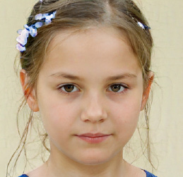
Figure 6.1 – Fake face generation using StyleGAN (image credit – https://thispersondoesnotexist.com)
Creating such incredibly realistic faces is one of the most successful use cases of GANs. However, GANs are not limited to just generating pretty faces or deepfake videos; they also have key commercial applications as well, such as generating images of houses or creating new models of cars or paintings.
While generative models have been used in the past in statistics, deep generative models such as GANs are relatively new. Deep generative models also include Variational Autoencoders (VAEs) and auto-regressive models. However, with GAN being the most popular method, we will focus on them here.
What is a GAN?
Interestingly, GAN originated not as a method of generating new things but as a way to improve the accuracy of vision models for recognizing objects. Small amounts of noise in the dataset can make image recognition models give wildly different results. While researching methods on how to thwart adversarial attacks on Convolutional Neural Network (CNN) models for image recognition, Ian Goodfellow and his team at Google came up with a rather simple idea. (There is a funny story about Ian and his team discovering GANs, involving a lot of beer and ping-pong, which every data scientist who also loves to party may be able to relate to!)
Every CNN type of model takes an image and converts it into a lower-dimensional matrix that is a mathematical representation of that image (which is a bunch of numbers to capture the essence of the image). What if we do the reverse? What if we start with a mathematical number and try to reconstruct the image? Well, it may be hard to do so directly, but by using a neural network, we can teach machines to generate fake images by feeding them with lots of real images, their representations in numbers, and then create some variation of those numbers to get a new fake image. That is precisely the idea behind a GAN!
A typical GAN architecture consists of three parts – the generator, discriminator, and comparison modules:
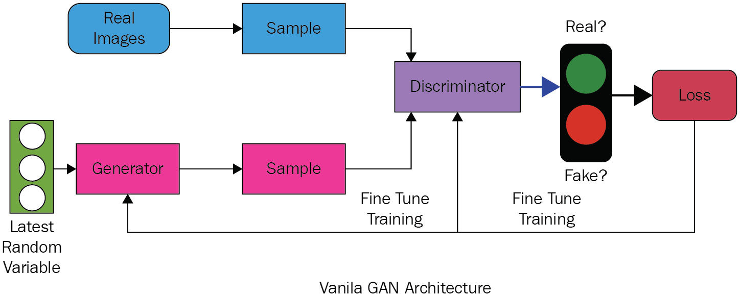
Figure 6.2 – Vanilla GAN architecture
Both the generator and the discriminator are neural networks. We start with real images and, using an encoder, convert them into a lower-dimensional entity. Both the generator and the discriminator participate in a play-off, trying to beat each other. The job of the generator is to generate a fake image using random mathematical values (which is a combination of real values plus some random noise) and the job of the discriminator is to determine whether it's real or fake. A loss function acts as a measure of who is winning the play-off. As loss is reduced by running through various epochs, the overall architecture is getting better at generating realistic images.
The success of GANs relies mostly on the fact that they use a very small number of parameters and thereby can give amazing results, even with a small amount of data. There are many variants of a GAN, such as a StyleGAN and a BigGAN, each with different neural network layers; however, they all follow the same architecture. The preceding image of a fake girl uses the StyleGAN variant.
Creating new food items using a GAN
GANs are one of the most common and powerful algorithms used in generative modeling. GANs are used widely to generate fake faces, pictures, anime/cartoon characters, image style translations, semantic image translation, and so on.
We will start by creating an architecture for our GAN model:
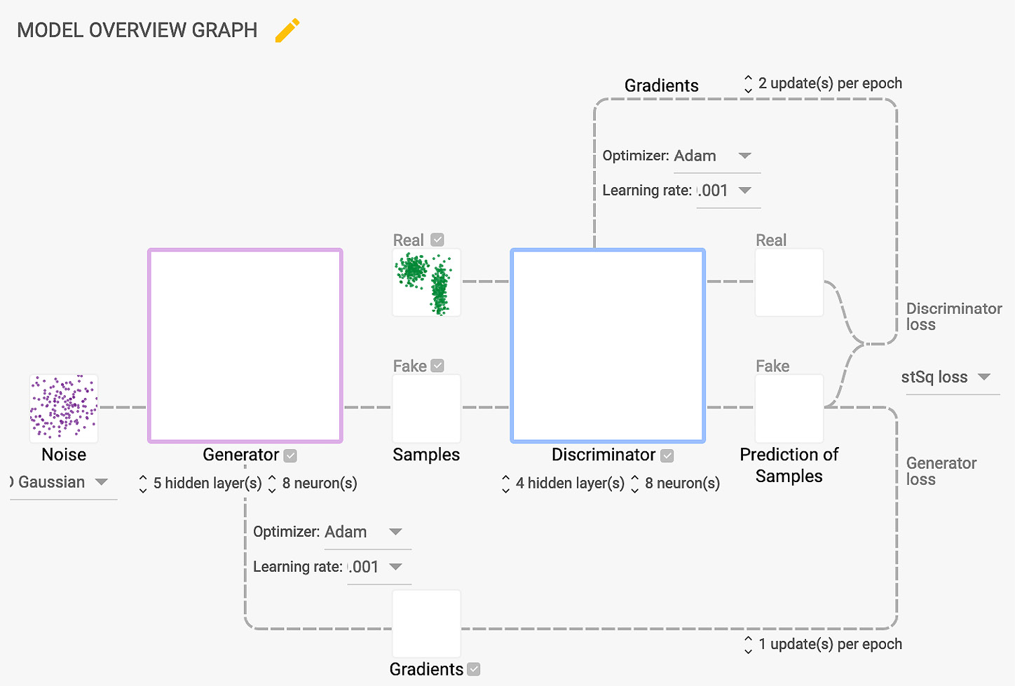
Figure 6.3 – GAN architecture for creating a new food
Firstly, we will define the neural networks for the generator and the discriminator with multiple layers of convolution and fully connected layers. In the architecture that we will be building, we will have four convolutional and one fully connected layer for the discriminator, and we will be utilizing five transposed convolution layers for the generator. We will attempt to generate fake images by adding Gaussian noise and use the discriminator to detect these fake images. Then, we will use the Adam optimizer to optimize the neural network. For this use, we will use cross-entropy loss to minimize the loss function.
There are several other hyperparameters such as image size, batch size, latent size, learning rate, channel, kernel size, stride, and padding that are also optimized to get output from the GAN model. These parameters can be fine-tuned as per the model configuration. The goal here is to train a GAN model architecture with the food dataset and generate fake food images and, similarly, use the same GAN model architecture with the butterfly dataset to generate fake butterfly images. We will save the generated images at the end of every epoch to compare new food or butterfly images at every epoch.
In this section, we're going to cover the following main steps to generate fake food images:
- Load the dataset.
- Feature-engineer the utility functions.
- Configure the discriminator model.
- Configure the generator model.
- Configure the generative adaptive model.
- Train the GAN model.
- Get output for the fake food images.
Loading the dataset
The dataset contains 16,643 food images, grouped in 11 major food categories. This dataset can be downloaded from Kaggle with this URL: https://www.kaggle.com/trolukovich/food11-image-dataset.
The code for downloading the dataset is shown here:
dataset_url = 'https://www.kaggle.com/trolukovich/food11-image-dataset'
od.download(dataset_url)
In the preceding code, we are using the download method from the opendatasets package to download the dataset into our Colab environment.
The total size of the food dataset is 1.19 GB and the dataset has three subfolders – training, validation, and evaluation. Each subfolder has food images stored in the nested subfolder under the 11 major food categories. For this chapter, to build our GAN model, we shall be training our model on the training images, so we will use only the training subfolder. All the images are colored and stored in the nested subfolders with respect to their food category.
Here are some of the sample images of food from the dataset:

Figure 6.4 – Original random images of food from the dataset
Data processing is always the most important step for any model. So, we will carry out some transformations on the input image data for our GAN model to perform better and faster. In this use case, we will focus primarily on the four major transformations, as shown in the following steps:
- Resize: First, we shall resize the images to 64 pixels.
- Center crop: Then, we will crop the resized image in the center. This converts our images to squares. Center crop is a critical transformation for our GAN model to perform better.
- Convert to tensors: Once the image has been resized and center-cropped, we shall convert the image data to tensor so that it can be processed in the GAN model.
- Normalize: Finally, we shall normalize the tensors in the range of -1 to 1 with a mean of 0 and a standard deviation of 0.5.
- All of the preceding transformations will not only help our GAN model to perform better but also reduce the training time significantly.
Important Note
There are many other transformations you can try to improve the model performance, but for this use case, the preceding transformations are good enough to start with.
The following code snippet shows some of the key configurations for our GAN model:
image_size = 64
batch_size = 128
normalize = [(0.5, 0.5, 0.5), (0.5, 0.5, 0.5)]
latent_size = 256
food_data_directory = "/content/food11-image-dataset/training"
In the preceding code, we are first initializing the variables to be used in the next step. The image size is set to 64 pixels, the batch size is 128, and the mean and standard deviation for normalizing the tensors are both 0.5. The latent size is set to 256, and the path to the food training images is saved as food_data_directory. In the next step, we will use these variables to transform our input images to prepare it for our GAN model:
food_train_dataset = ImageFolder(food_data_directory, transform=T.Compose([
T.Resize(image_size),
T.CenterCrop(image_size),
T.ToTensor(),
T.Normalize(*normalize)]))
food_train_dataloader = DataLoader(food_train_dataset, batch_size, num_workers=4, pin_memory=True, shuffle=True)
In the preceding code, we are using the ImageFolder class from the torchvision.datasets library to load the images dataset. We are using the Compose method from the torchvision.transforms library to compose several transformations together. Inside the compose method, the first step is the Resize method to set the image size to 64 pixels. In the next transform, we are using the CenterCrop method to convert the image into a square. Then, we are converting the resized and cropped image to tensors and, finally, normalizing them between -1 and 1 with a mean and standard deviation of 0.5. We are saving these transformed images in food_train_dataset. In the final step, we are using the DataLoader class from torch.utils.data library to create food_train_dataloader with a batch size of 128 and 4 workers, and setting up some of the parameters to make the data loader work better.
So far, in the preceding code, we have loaded our dataset and performed some of the transformations, and food_train_dataloader is ready with images in batches of 128.
In the data processing step, we are transforming and normalizing our images, so it is important for us to bring them back to their original form by denormalizing them. We also need to compare the images generated by our GAN model for each epoch, so we need to save the images at the end of every epoch. Therefore, we will write some utility functions to make these happen in the following section of this chapter.
Feature engineering utility functions
Let's go through the two main functions that are important to understand.
The first utility function that we need is to denormalize the images back to the original form. The denormalize utility function is shown here:
def denormalize(input_image_tensors):
input_image_tensors = input_image_tensors * normalize[1][0]
input_image_tensors = input_image_tensors + normalize[0][0]
return input_image_tensors
The denormalize utility function takes in the tensors and denormalizes them by multiplying by 0.5 and then adding 0.5. These normalization values (mean and standard deviation) are defined at the beginning of this section.
The second utility function required is for saving the images at the end of every epoch. The following is the code snippet for the second utility function:
def save_samples(index, sample_images):
fake_fname = 'generated-images-{}.png'.format(index)
save_image(denormalize(sample_images[-64:]), os.path.join(".", fake_fname), nrow=8)
The save_samples utility function takes the index, which is the epoch number, and sample_images, which is the image returned by the GAN model at the end of every epoch, as input. Then, it saves the last 64 images in a grid of 8 x 8.
Important Note
In this function, there is a total of 128 images in the same batch input passed, but we are saving only the last 64 images. You can easily change this to save fewer or more images. More images typically require more compute (GPU) power and memory.
We also have other utility functions used in the chapter, which can be found in the full notebook of the GitHub page for our book.
The discriminator model
As mentioned previously, the discriminator in a GAN is a classifier that tries to distinguish real data from the data created by the generator. In this use case, the discriminator acts as a binary classification for the images classifying the images between real and fake classes.
Defining parameters
Let's start by creating a class called FoodDiscriminator that is inheriting from the PyTorch nn module. Some of the important features/attributes for the Discriminator class are shown in the following code snippet:
class FoodDiscriminator(nn.Module):
def __init__(self, input_size):
super().__init__()
self.input_size = input_size
self.channel = 3
self.kernel_size = 4
self.stride = 2
self.padding = 1
self.bias = False
self.negative_slope = 0.2
The input for FoodDiscriminator is the output generated from the generator, which is sized 3 x 64 x 64. We are also setting some of the variables, such as a channel size of 3, a kernel size of 4, a stride of 2, padding of 1, a bias of False, and a negative slope value of 0.2.
The input channel is set to 3, since we have color images, and the 3 channel represents red, green, and blue. The kernel size is 4, which represents the height and width of the 2D convolution window. The stride with the 2 value moves the kernel two steps when performing convolutions. The padding adds a 1-pixel layer to all the boundaries of the images. Setting the bias to False means that it is not allowing the convolution network to add any learnable bias to the network.
The negative_slope is set to 0.2, which controls the angle of the negative slope for the LeakyReLU activation function. We will be using Leaky ReLU for the activation function here. There are multiple activation functions available, such as ReLU, tan-h, and sigmoid, but discriminators perform better with the Leaky ReLU activation function. The difference between a ReLU activation function and the Leaky ReLU activation function is that the ReLU function allows only positive values as output, whereas Leaky ReLU allows negative values as output. We are allowing 0.2 times the negative value as the output of the Leaky ReLU activation function by setting the value in negative_slope.
Building convolutional layers
Now, we will define the layers of the discriminator to build our binary classification model.
The following is the code snippet for the layers of the discriminator model:
#input size: (3,64,64)
self.conv1 = nn.Conv2d(self.channel, 128, kernel_size=self.kernel_size, stride=self.stride, padding=self.padding, bias=self.bias)
self.bn1 = nn.BatchNorm2d(128)
self.relu = nn.LeakyReLU(self.negative_slope, inplace=True)
#input size: (64,32,32)
self.conv2 = nn.Conv2d(128, 256, kernel_size=self.kernel_size, stride=self.stride, padding=self.padding, bias=self.bias)
self.bn2 = nn.BatchNorm2d(256)
#input size: (128,16,16)
self.conv3 = nn.Conv2d(256, 512, kernel_size=self.kernel_size, stride=self.stride, padding=self.padding, bias=self.bias)
self.bn3 = nn.BatchNorm2d(512)
#input size: (256,8,8)
self.conv4 = nn.Conv2d(512, 1024, kernel_size=self.kernel_size, stride=self.stride, padding=self.padding, bias=self.bias)
self.bn4 = nn.BatchNorm2d(1024)
# nn.LeakyReLU(self.negative_slope, inplace=True)
self.fc = nn.Sequential(
nn.Linear(in_features=16384,out_features=1),
# nn.Flatten(),
nn.Sigmoid()
)
In the preceding code, we are defining the layers of the discriminator model to build a binary classification model that takes in output from the generator model, which is an image with a size of 3 x 64 x 64 and generates output of either 0 or 1. Thus, the discriminator is able to identify whether an image is fake or real.
The discriminator model shown previously consists of four convolutional layers and a fully connected layer, where the first layer takes in an image generated from the generator model, and each consecutive layer takes in input from the previous layer and passes output to the next layer.
We will split this code block into sections to understand it better. Let's talk more about each layer in detail.
The first convolutional layer
The following is the code snippet for our first convolution layer:
#input size: (3,64,64)
self.conv1 = nn.Conv2d(self.channel, 128, kernel_size=self.kernel_size, stride=self.stride, padding=self.padding, bias=self.bias)
self.bn1 = nn.BatchNorm2d(128)
self.relu = nn.LeakyReLU(self.negative_slope, inplace=True)
The first layer, conv1, takes the image generated by the generator as input, which is of the size 3 x 64 x 64, with a kernel size of 4, the stride as 1, a padding of 1 pixel, and bias = False. The conv1 layer then generates an output of 128 channels, each with a size of 32 – that is, 128 x 32 x 32. Then, the convolution output is normalized using batch normalization, which helps convolutional networks to perform better. Finally, we are using Leaky ReLU as our activation function in the final step of the first layer.
The second convolutional layer
The following is the code snippet for our second convolution layer:
#input size: (128,32,32)
self.conv2 = nn.Conv2d(128, 256, kernel_size=self.kernel_size, stride=self.stride, padding=self.padding, bias=self.bias)
self.bn2 = nn.BatchNorm2d(256)
self.relu = nn.LeakyReLU(self.negative_slope, inplace=True)
In the preceding code, we have defined the second convolution layer, conv2, which takes in output of the first convolution layer, which is of the size 128 x 32 x 32 with the same kernel size, stride, padding, and bias as the first layer. Now, this layer generates output with 256 channels, each with a size of 16 – that is, 256 x 16 x 16 – and passes it to batch normalization. Again, we are using Leaky ReLU as our activation function in the final step of the second layer.
The third convolutional layer
The following is the code snippet for our third convolution layer:
#input size: (256,16,16)
self.conv3 = nn.Conv2d(256, 512, kernel_size=self.kernel_size, stride=self.stride, padding=self.padding, bias=self.bias)
self.bn3 = nn.BatchNorm2d(512)
self.relu = nn.LeakyReLU(self.negative_slope, inplace=True)
The third convolution layer, self.conv3, takes in the output from the second layer as input, which is of the size 256 x 16 x 16 with the same kernel size, stride, padding, and bias as the first two convolution layers. This layer applies convolution to generate output with 512 channels, each with a size of 8 – that is, 512 x 8 x 8 – and passes it to batch normalization. Again, we are using Leaky ReLU as our activation function in the final step of the third layer.
The fourth convolutional layer
The following is the code snippet for our fourth convolution layer:
#input size: (512,8,8)
self.conv4 = nn.Conv2d(512, 1024, kernel_size=self.kernel_size, stride=self.stride, padding=self.padding, bias=self.bias)
self.bn4 = nn.BatchNorm2d(1024)
self.relu = nn.LeakyReLU(self.negative_slope, inplace=True)
The fourth convolution layer, self.conv4, takes in output from the third layer as input, which is of the size 512 x 8 x 8 with the same kernel size, stride, padding, and bias as the first three convolution layers. This layer applies convolution to generate output with 1,024 channels, each with a size of 4 – that is, 1,024 x 4 x 4 – and passes it to batch normalization. Again, we are using Leaky ReLU as our activation function in the final step of the fourth layer.
The fifth fully connected layer (final layer)
The following is the code snippet for our final fully connected layer:
self.fc = nn.Sequential(
nn.Linear(in_features=16384,out_features=1),
nn.Sigmoid()
)
# output size: 1 x 1 x 1
The final layer of the discriminator model as shown previously is built using the sequential function. There is a fully connected layer in this final layer that takes in the output from the fourth layer, which is of the size 1,024 x 4 x 4. So, the total number of features for a fully connected linear layer is 16,384. Since this is a binary classification task, the final fully connected layer will generate output with 1 channel each of size 1 – that is, of size 1 x 1 x 1. This output is then passed to the sigmoid activation function, which generates output between 0 and 1, and helps the discriminator to work as a binary classification model.
To summarize, we have defined the layers of our discriminator model as a combination of convolutional layers and fully connected linear networks. These layers will take an image generated from the generator as input to classify them between fake or real. Now, it's time to pass in data from the different layers and activation functions. This can be achieved by overwriting the forward method. The code for the forward method of the FoodDiscriminator class is shown here:
def forward(self, input_img):
validity = self.conv1(input_img)
validity = self.bn1(validity)
validity = self.relu(validity)
validity = self.conv2(validity)
validity = self.bn2(validity)
validity = self.relu(validity)
validity = self.conv3(validity)
validity = self.bn3(validity)
validity = self.relu(validity)
validity = self.conv4(validity)
validity = self.bn4(validity)
validity = self.relu(validity)
validity=validity.view(-1, 1024*4*4)
validity=self.fc(validity)
return validity
In the preceding code, we have the following:
- We pass the data (the image output from the generator model) in our first convolution layer (self.conv1). The output from self.conv1 is passed to the batch normalization function, self.bn1, and the output from the batch normalization function is passed to the Leaky ReLU activation function, self.relu.
- Then, the output is passed to the second convolution layer (self.conv2). Again, the output from the second convolution layers is passed to the batch normalization function, self.bn2, and then to the Leaky ReLU activation function, self.relu.
- Similarly, the output is now passed to the third convolution layer (self.conv3). And, as with the first two convolution layers, this output is passed to the batch normalization function, self.bn3, and then to the leaky ReLU activation function, self.relu.
- The same pass is repeated for the fourth convolution layer (self.conv4), batch normalization function (self.bn4), and leaky ReLU activation (self.relu).
- Data is passed through the convolution layer, and the output from these layers is multidimensional. To pass the output to our linear layer, it is converted to single-dimensional form. This can be achieved using the tensor view method.
- Once the data is ready in single-dimensional form, it is passed over the fully connected layer, and the final output is returned, which is binary 1 or 0.
To reiterate, in the forward method, the image data which is the output from the generator is first passed over the four convolution layers, and then output from the convolution layers is passed over one fully connected layer. Finally, the output is returned.
Important Note
The activation function that we have used in our discriminator model is Leaky ReLU, which tends to perform better and helps the GAN to perform better.
Now that we have completed the discriminator part of the architecture, we will move toward building the generator.
The generator model
As mentioned in the introduction, the role of the generator part of a GAN is to create fake data (images in this case) by incorporating feedback from the discriminator. The goal of the generator is to generate fake images that are very close to real images so that the discriminator fails to recognize them as fake images.
Let's start by creating a class called FoodGenerator that is inheriting from the PyTorch nn module. Some of the important features/attributes for the FoodGenerator class are shown in the following code snippet:
class FoodGenerator(nn.Module):
def __init__(self, latent_size = 256):
super().__init__()
self.latent_size = latent_size
self.kernel_size = 4
self.stride = 2
self.padding = 1
self.bias = False
The latent size is one of the most important features in the generator model. It represents the compressed low-dimensional representation of the input (food images, in this case) and is set to 256 by default here. Then, we set the kernel size to be 4 with a stride of 2, which moves the kernel by two steps when performing convolutions. We are also setting the padding to 1, which adds one additional pixel to all boundaries of the food images. Finally, the bias is set to False, which means it does not allow the convolution network to add any learnable bias to the network.
We will use the Sequential function from the neural network module of the torch library (torch.nn) to build the layers of our generator model. The following is the code snippet for building the generator model:
self.model = nn.Sequential(
#input size: (latent_size,1,1)
nn.ConvTranspose2d(latent_size, 512, kernel_size=self.kernel_size, stride=1, padding=0, bias=self.bias),
nn.BatchNorm2d(512),
nn.ReLU(True),
#input size: (512,4,4)
nn.ConvTranspose2d(512, 256, kernel_size=self.kernel_size, stride=self.stride, padding=self.padding, bias=self.bias),
nn.BatchNorm2d(256),
nn.ReLU(True),
#input size: (256,8,8)
nn.ConvTranspose2d(256, 128, kernel_size=self.kernel_size, stride=self.stride, padding=self.padding, bias=self.bias),
nn.BatchNorm2d(128),
nn.ReLU(True),
#input size: (128,16,16)
nn.ConvTranspose2d(128, 64, kernel_size=self.kernel_size, stride=self.stride, padding=self.padding, bias=self.bias),
nn.BatchNorm2d(64),
nn.ReLU(True),
nn.ConvTranspose2d(64, 3, kernel_size=self.kernel_size, stride=self.stride, padding=self.padding, bias=self.bias),
nn.Tanh()
# output size: 3 x 64 x 64
)
In the preceding code, we are defining the layers of the generator model to generate fake images sized 3 x 64 x 64. The generator model shown previously consists of five deconvolutional layers where each layer takes in input and passes output to the next layer.
The generator model is almost the opposite of the layers of the discriminator model, except for a fully connected linear layer.
Comparing Transposed Convolution and Deconvolution
The two terms are often used interchangeably in the Deep Learning community, and that is the case in this book. Mathematically speaking, deconvolution is a mathematical operation that reverses the effect of convolution. Imagine throwing an input through a convolutional layer and collecting the output. Now, throw the output through the deconvolutional layer, and you get back the exact same input. It is the inverse of the multivariate convolutional function.
What we are doing here is not getting back the exact same input. So, while the operation is similar, it is strictly speaking NOT deconvolution but transposed convolution. A transposed convolution is somewhat similar because it produces the same spatial resolution as a hypothetical deconvolutional layer would. However, the actual mathematical operation that's being performed on the values is different. A transposed convolutional layer carries out a regular convolution but reverses its spatial transformation.
Deconvolution, as discussed, is not very popular, and often, the community refers to transposed convolution as deconvolution, which is what is being referred to here.
We will split this code block into sections to understand it better. Let's talk more about each layer in detail.
The first transposed convolution layer
Here is the code snippet for our first ConvTranspose2d layer:
#input size: (latent_size,1,1)
nn.ConvTranspose2d(latent_size, 512, kernel_size=self.kernel_size, stride=1, padding=0, bias=self.bias),
nn.BatchNorm2d(512),
nn.ReLU(True),
The first ConvTranspose2d layer takes latent_size as input, which is 256, with a kernel size of 4, the stride as 1, a padding of 0 pixels, and bias = False. The ConvTranspose2d layer then generates an output of 512. Then, the transposed convolution output is normalized using batch normalization, which helps transposed convolutional networks to perform better. Finally, we are using ReLU as our activation function in the final step of the first layer.
The second transposed convolution layer
The following is the code snippet for our second ConvTranspose2d layer:
#input size: (512,4,4)
nn.ConvTranspose2d(512, 256, kernel_size=self.kernel_size, stride=self.stride, padding=self.padding, bias=self.bias),
nn.BatchNorm2d(256),
nn.ReLU(True),
In the preceding code, we have defined the second transposed convolution layer that takes in the output of the first transposed convolution layer, which is sized 512 x 4 x 4, with a kernel size of 4, the stride as 2, a padding of 1 pixel, and bias = False. Now, this layer generates output with 256 channels and passes it to batch normalization. Again, we are using ReLU as our activation function in the final step of the second layer.
The third transposed convolution layer
The following is the code snippet for our third ConvTranspose2d layer:
#input size: (256,8,8)
nn.ConvTranspose2d(256, 128, kernel_size=self.kernel_size, stride=self.stride, padding=self.padding, bias=self.bias),
nn.BatchNorm2d(128),
nn.ReLU(True),
The third transposed convolution layer takes in the output from the second layer as input, which is sized 256 x 8 x 8, with the same kernel size, stride, padding, and bias as the second transposed convolution layers. This layer applies transposed convolution to generate output with 128 channels and passes it to batch normalization. Again, we are using ReLU as our activation function in the final step of the third layer.
The fourth transposed convolution layer
The following is the code snippet for our fourth ConvTranspose2d layer:
#input size: (128,16,16)
nn.ConvTranspose2d(128, 64, kernel_size=self.kernel_size, stride=self.stride, padding=self.padding, bias=self.bias),
nn.BatchNorm2d(64),
nn.ReLU(True),
The fourth transposed convolution layer takes in the output from the third layer as input, which is sized 128 x 16 x 16, with the same kernel size, stride, padding, and bias as the last two transposed convolution layers. This layer applies transposed convolution to generate output with 64 channels and passes it to batch normalization. Again, we are using ReLU as our activation function in the final step of the fourth layer.
The fifth transposed convolution layer (final layer)
The following is the code snippet for our fifth and final ConvTranspose2d layer:
nn.ConvTranspose2d(64, 3, kernel_size=self.kernal_size, stride=self.stride, padding=self.padding, bias=self.bias),
nn.Tanh()
# output size: 3 x 64 x 64
In the final deconvolution neural network layer, we are generating output with 3 channels of 64 x 64 size and with the activation function as Tanh. Here, we are using a different activation function because this is a generator model, which works better with Tanh.
Note that for the first transposed convolutional layer, we are using a stride of 1 and no padding, while for the rest of the layers, we are using padding sized 1 and with a stride of 2.
To summarize, we have defined the layers of our generator model as five transposed convolutional layers. These layers will take in latent size as input, go through multiple deconvolutional layers, and scale up the channels from 256 to 512, then down to 256 to 128, and finally, to 3 channels.
Now, it's time to pass in the data from the different layers and the activation functions. This can be achieved by overwriting the forward method. The code for the forward method of the FoodGenerator class is shown here:
def forward(self, input_img):
input_img = self.model(input_img)
return input_img
In the preceding code, the forward method of the FoodGenerator class takes in the image as input, passes it to the model, which is a sequence of the transposed convolutional layer, and returns the output, which is the generated fake image.
The generative adversarial model
Now that we have defined our discriminator and generator models, it's time to combine them and build our GAN model. We shall be configuring the loss function and optimizer in the GAN model and passing the data to the generator and the discriminator. In order to get good results (which means generating fake images that are as good-looking as real images), we will try to minimize the loss. Let's look at the PyTorch Lightning implementation for GANs in detail.
Building our GAN model using PyTorch Lightning primarily includes the following steps:
- Define the model.
- Configure the optimizer and loss function.
- Configure the training loop.
- Save the generated fake images.
- Train the GAN model.
Let's look at these steps in detail.
Defining the model
Let's create a class called FoodGAN that is inherited from a PyTorch LightningModule. The Module class takes the following parameters in the constructor:
- latent_size: This represents the compressed low-dimensional representation of the food images. The default value is 256.
- lr: This is the learning rate for the optimizers used for both the discriminator and the generator. The default value is 0.0002.
- bias1 and bias2: b1 and b2 are the bias values used for the optimizers for both the discriminator and the generator. The default value for b1 is 0.5, and for b2, it is 0.999.
- batch_size: This represents the number of images that will be propagated through the network. The default value for the batch size is 128.
Now, we will initialize, configure and construct our FoodGAN class using the __init__ method. The following is the code snippet for the __init__ method:
def __init__(self, latent_size = 256,learning_rate = 0.0002,bias1 = 0.5,bias2 = 0.999,batch_size = 128):
super().__init__()
self.save_hyperparameters()
# networks
# data_shape = (channels, width, height)
self.generator = FoodGenerator()
self.discriminator = FoodDiscriminator(input_size=64)
self.batch_size = batch_size
self.latent_size = latent_size
self.validation = torch.randn(self.batch_size, self.latent_size, 1, 1)
The __init__ method defined previously takes in the latent size, learning rate, bias1, bias2, and the batch size as input. These are all the hyperparameters required for the discriminator and generator models, so these variables are saved inside the __init__ method. Finally, we are also creating a variable called validation, which we will use for the validation of the model.
Configuring the optimizer and loss function
We shall also define a utility function in the FoodGAN model to calculate loss, as explained in the previous section, since we want to minimize the loss to get better results. The following is the code snippet for the loss function:
def adversarial_loss(self, preds, targets):
return F.binary_cross_entropy(preds, targets)
In the preceding code snippet, the adversarial_loss method takes in two parameters – preds, which is the predicted value, and targets, which is the real target values. Then, it uses a binary_cross_entropy function to calculate the loss from the predicted value and the target value and, finally, returns the entropy value calculated.
Important Note
It is also possible to have different loss functions for the generator and the discriminator. Here, we kept things simple and only used binary cross-entropy loss.
The next important method is for configuring optimizers, since we have two models, the discriminator and the generator, in the FoodGAN model, and each model needs its own optimizers. This can be easily achieved using one of the PyTorch Lightning life cycle methods, called configure_optimizer. The following is the code snippet for the configure_optimizer method:
def configure_optimizers(self):
learning_rate = self.hparams.learning_rate
bias1 = self.hparams.bias1
bias2 = self.hparams.bias2
opt_g = torch.optim.Adam(self.generator.parameters(), lr=learning_rate, betas=(bias1, bias2))
opt_d = torch.optim.Adam(self.discriminator.parameters(), lr=learning_rate, betas=(bias1, bias2))
return [opt_g, opt_d], []
In the __init__ method, we have invoked a method called self.save_hyperparameters(). This saves all the input sent to the init method to a special variable called hparams. This special variable is leveraged in the configure_optimizer method to access our learning rate and the bias values. Here, we are creating two optimizers – opt_g is the optimizer for the generator and opt_d is the optimizer for the discriminator, as each of them needs its own optimizer. The configure optimizer method returns two lists – the first list contains multiple optimizers and the second list, which is empty in our case, is where we can pass LR schedulers.
To summarize, we are creating two optimizers, one for the generator and one for the discriminator, by accessing hyperparameters from the hparams special variable. This method returns two lists as output, where the first element of the first list is the optimizer for the generator and the second element is the optimizer for the discriminator.
Important Note
The configure_optimizer method returns two values; both are a list, and out of them, the second is an empty list. The list has two values – the value at the 0 index has an optimizer for the generator, and the value at the 1 index has an optimizer for the discriminator.
Another important life cycle method is the forward method. The following is the code snippet for this method:
def forward(self, z):
return self.generator(z)
In the preceding code, the forward method takes in input, passes it to the generator model, and returns the output.
Configuring the training loop
We have overwritten the method to configure optimizers for the discriminator and generator models. Now, it's time to configure the training loop for the discriminator and the generator. It is important to access the correct optimizer for the discriminator and generator during the training of the GAN model, which can be done by using data that is being passed as input by the PyTorch Lightning module during training. Let's try to understand more about the input passed for the training life cycle method and training process in detail.
The following inputs are passed to the training_step life cycle methods:
- batch: This represents batch data that is being served by food_train_dataloader.
- batch_idx: This is the index of the batch that is being served for training.
- optimizer_idx: This helps us to identify the two different optimizers for the generator and the discriminator. This input parameter has two values, 0 for the generator and 1 for the discriminator.
Training the generator model
Now that we understand how we can identify the optimizers for the discriminator and the generator, it's time to understand how to train our GAN model using both of them. The code snippet for training the generator is as follows:
real_images, _ = batch
# train generator
if optimizer_idx == 0:
# Generate fake images
fake_random_noise = torch.randn(self.batch_size, self.latent_size, 1, 1)
fake_random_noise = fake_random_noise.type_as(real_images)
fake_images = self(fake_random_noise) #self.generator(latent)
# Try to fool the discriminator
preds = self.discriminator(fake_images)
targets = torch.ones(self.batch_size, 1)
targets = targets.type_as(real_images)
loss = self.adversarial_loss(preds, targets)
self.log('generator_loss', loss, prog_bar=True)
tqdm_dict = {'g_loss': loss}
output = OrderedDict({
'loss': loss,
'progress_bar': tqdm_dict,
'log': tqdm_dict
})
return output
In the preceding code, we are first storing the images received from the batch in a variable called real_images. These inputs are in tensor format. It is important to make sure all the tensors are making use of the same device – in our case, the GPU, so that it can run on the GPUs. In order to convert all the tensors to the same type so that they are pointing it to the same device, we are leveraging the PyTorch Lightning-recommended method called type_as(). The type_as method will convert the tensor to the same type as the others to make sure that all the tensor types are the same and can make use of the GPUs, while also making our code scale to any arbitrary number of GPUs or TPUs. More information about this method can be found in the PyTorch Lightning documentation.
As we discussed in the previous section, it is important to identify the optimizer for the generator to train our generator model. We are identifying the optimizer for the generator by checking optimizer_idx, which has to be 0 for the generator. There are three main steps in training the generator model – creating random noise data, converting the type of the random noise, and generating fake images from random noise. The following is the code snippet demonstrating this:
fake_random_noise = torch.randn(self.batch_size, self.latent_size, 1, 1)
fake_random_noise = fake_random_noise.type_as(real_images)
fake_images = self(fake_random_noise)
In the preceding code, the following steps are carried out:
- The first step is to create some random noise data. In order to create random noise data, we are leveraging the randn method from the torch package, which returns a tensor filled with random numbers of size equal to the latent size. This random noise is saved as the fake_random_noise variable.
- The next step is converting the tensor type of the random noise to the same as our real_images tensor. This is achieved by the type_as method described previously.
- Finally, the random noise is passed to the self-object, which is passing the random noise data to our generator model to generate fake images. These are saved as fake_images.
Since we have generated our fake image now, the next step is to calculate the loss. However, it is important to identify how close our fake image is to the real image before calculating loss. We have already defined our discriminator and can easily leverage it to identify this by passing our fake image to the discriminator and comparing the output. So, we shall pass the fake image generated in the preceding step to our discriminator and save the predictions, where the values can be either 0 or 1. The following code snippet shows how to pass the fake images to the discriminator:
# Try to fool the discriminator
preds = self.discriminator(fake_images)
targets = torch.ones(self.batch_size, 1)
targets = targets.type_as(real_images)
In the preceding code, we are first passing the fake images to the discriminator and saving them in the variable preds. Then, we are creating a target variable with all but one, assuming that all the images generated by the generator are the real images. This will start improving after a few epochs as the GAN model is being trained. Finally, we are converting the type of the tensors for the targets to the same type as our real_images tensors.
In the next step, we shall calculate the loss. This is achieved by using our adversarial_loss utility function, as shown here:
loss = self.adversarial_loss(preds, targets)
self.log('generator_loss', loss, prog_bar=True)
The adversarial_loss method takes in the predicted values from the discriminator and the target values, which are all ones as the input and calculates loss. The loss is logged as generator_loss, which is important if you want to plot the loss using TensorBoard later.
Finally, we shall return the loss function and other attributes to make use of the loss being logged and shown on the progress bar, as shown here:
tqdm_dict = {'g_loss': loss}
output = OrderedDict({
'loss': loss,
'progress_bar': tqdm_dict,
'log': tqdm_dict
})
return output
In the preceding code, the loss and other attributes are stored in the dictionary called output, and this is returned in the final step of training the generator. Once this loss value is returned in the training step, PyTorch Lightning will take care of updating weights.
Training the discriminator model
Now, let's try to understand how to train our discriminator model.
Similar to the generator model, we will begin by comparing the optimizer index and train the discriminator only when the index is 1, as shown here:
# train discriminator
if optimizer_idx == 1:
There are four steps that we will follow to train our discriminator model – train our discriminator to identify the real images, save the output of the discriminator model, convert the type of the tensors for the output of the discriminator, and calculate the loss. These steps are achieved by the code snippet shown here:
real_preds = self.discriminator(real_images)
real_targets = torch.ones(real_images.size(0), 1)
real_targets = real_targets.type_as(real_images)
real_loss = self.adversarial_loss(real_preds, real_targets)
In the preceding code, we are first passing the real image to the discriminator and saving the output as real_preds. Then, we are creating a dummy tensor with the values as all ones, calling it real_targets. The reason for setting all our real target values to ones is that we are passing the real images to the discriminator. We are also converting the type of the tensor for the real targets to be the same as the tensors for the real images. Finally, we are calculating our loss and calling it real_loss.
Now, the discriminator has been trained with the real images, and it's time to train it with the fake images that are being generated by the generator model. This step is similar to training our generator. So, we will create dummy random noise data, pass it to the generator for creating fake images, and then pass it to the discriminator for classifying it. The processing of training the discriminator with fake images is shown in the following code snippet:
# Generate fake images
real_random_noise = torch.randn(self.batch_size, self.latent_size, 1, 1)
real_random_noise = real_random_noise.type_as(real_images)
fake_images = self(real_random_noise) #self.generator(latent)
# Pass fake images through discriminator
fake_targets = torch.zeros(fake_images.size(0), 1)
fake_targets = fake_targets.type_as(real_images)
fake_preds = self.discriminator(fake_images)
fake_loss = self.adversarial_loss(fake_preds, fake_targets)
# fake_score = torch.mean(fake_preds).item()
self.log('discriminator_loss', fake_loss, prog_bar=True)
In the preceding code, we are first generating fake images by following the same steps we followed while training the generator. These fake images are stored as fake_images.
Next, we are creating a dummy tensor with the values as all zeros, calling it fake_targets. Then, we are converting the type of tensors for fake_targets to be the same as the tensors for real_images. Then, we are passing the fake images through the discriminator to make predictions and saving the predictions as fake_preds. Finally, we are calculating the loss by leveraging the adversarial_loss utility function, which takes in fake_preds and fake_targets as input to calculate the loss. This is also logged in the self-object to be called later for plotting the loss function using TensorBoard.
The final step in training the GAN model after training the discriminator is to calculate the total loss, which is the sum of the loss calculated when training the discriminator with real images and the fake loss, which is the loss calculated when training the discriminator with fake images. The following is the code snippet demonstrating this:
# Update discriminator weights
loss = real_loss + fake_loss
self.log('total_loss', loss, prog_bar=True)
In the preceding code, we are adding real_loss and fake_loss to calculate the total loss and store it in the variable loss. This loss is also logged as the total loss to be called later for observation in TensorBoard.
Finally, we return the loss function and other attributes to log the loss values and show them in the progress bar. The following is the code snippet for returning loss and other attributes:
tqdm_dict = {'d_loss': loss}
output = OrderedDict({
'loss': loss,
'progress_bar': tqdm_dict,
'log': tqdm_dict
})
return output
In the preceding code, we are saving the loss function and other attributes in a dictionary called output, which is then returned at the end of the training. Once this loss value is returned in the training step, the PyTorch Lightning module will take care of updating the weights. This will complete our training configuration.
To summarize the training loop, we are first getting the optimizer index and then training either the generator or the discriminator based on the index value and, finally, returning the loss value as an output.
Important Note
When the optimizer_idx value is 0, the generator model is being trained, and when the value is 1, the discriminator model is being trained.
Saving the generated fake images
It is also important to check how well our GAN model is being trained and improving over epochs and see whether it can generate any new food dishes. We can track our GAN model at every epoch by saving some images at the end of each epoch. This can be achieved by leveraging one of the PyTorch Lightning methods called on_epoch_end(). This method is called at the end of every epoch, so we will use it to save fake images that the GAN model has generated. The following is the code demonstrating this:
def on_epoch_end(self):
# import pdb;pdb.set_trace()
z = self.validation.type_as(self.generator.model[0].weight)
sample_imgs = self(z) #self.current_epoch
ALL_FOOD_IMAGES.append(sample_imgs.cpu())
save_generated_samples(self.current_epoch, sample_imgs)
In the on_epoch_end() method, we are saving the weights of the generator model in the z variable and then using the self method to store the sample images as sample_imgs. Then, we are adding those sample images to the ALL_FOOD_IMAGES list. Finally, we are using our save_generated_samples utility function to save fake food images as .png files.
Training the GAN model
Finally, we are all set to train the GAN model. The following is the code for training our GAN model:
model = FoodGAN()
trainer = pl.Trainer( max_epochs=100, progress_bar_refresh_rate=25, gpus=1)#gpus=1,
trainer.fit(model, food_train_dataloader)
In the preceding code, we are first initializing our FoodGAN model, saving it as model. Then, we are calling the Trainer method from the PyTorch Lightning package with a maximum number of 100 epochs and 1 GPU enabled. Finally, we are using the fit method to start training by passing our FoodGAN model, along with the data loader created earlier in this section.
The following is the output of training the GAN model:
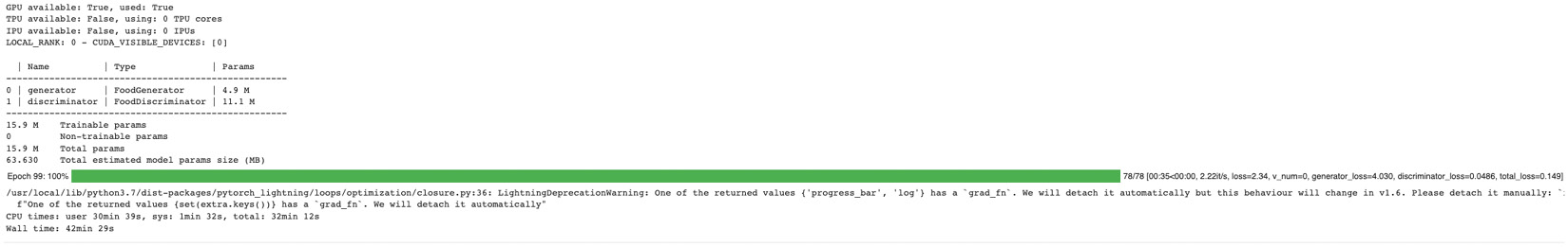
Figure 6.5 – Output of training the GAN model for 100 epochs
We can also visualize and observe the loss for the GAN model while it was training by leveraging TensorBoard, as shown here:
%load_ext tensorboard
%tensorboard --logdir lightning_logs/
This results in the following output:
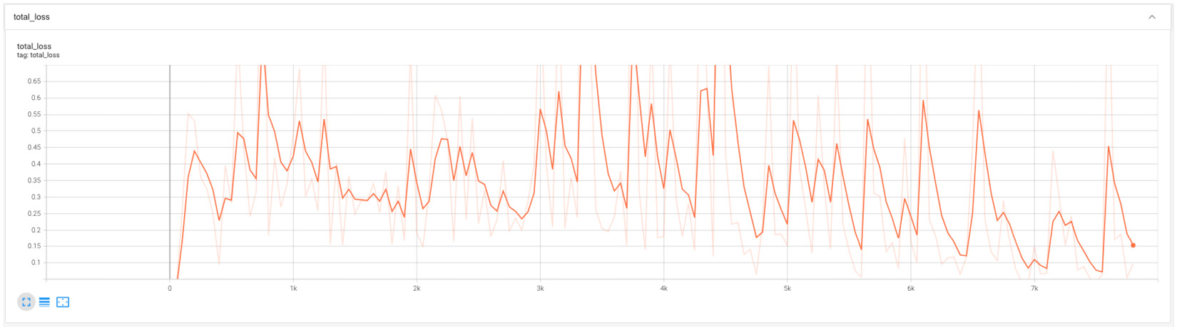
Figure 6.6 – Output for the total loss of the GAN model
We can also observe the generator loss and the discriminator loss (the full code and output is available in the GitHub repository).
The model output showing fake images
Here are some of the sample food images generated at different epochs.
We first train the model for 100 epochs but capture multiple results to show the progression:
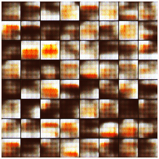
Figure 6.7 – The generated images after 3 epochs
The following figure shows the progress after 9 epochs:
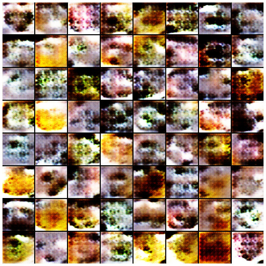
Figure 6.8 – The generated images after 9 epochs
The following figure shows the final output after 100 epochs:
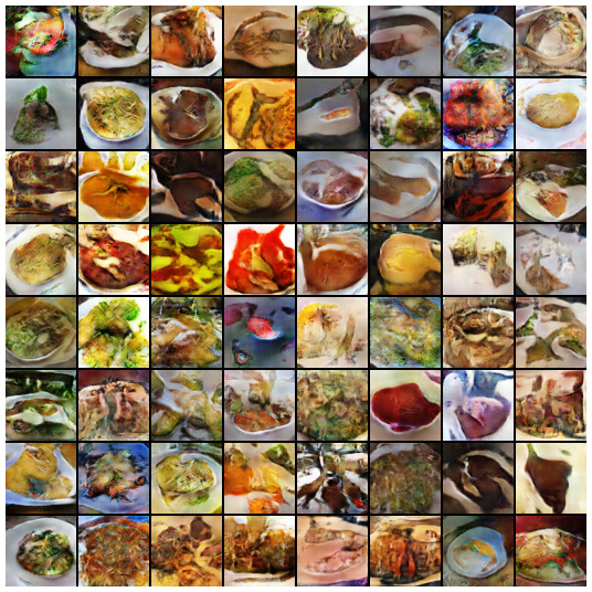
Figure 6.9 – The fake food images at epoch 100
As you can see, we now have some food that doesn't exist in the original dataset, so they are fake food (at least until now based on the dataset, so you can try making those at home).
You can train the model for a greater number of epochs and the quality will continue to improve. For example, try training for 200, 300, 400, and 500 epochs. (More results can be found on the GitHub page of our book.) There will always be some output that is completely noisy and looks like incomplete images.
A GAN is sensitive to batch size, latent size, and other hyperparameters. To improve the performance, you can try running the GAN model for a greater number of epochs and with different hyperparameters.
Creating new butterfly species using a GAN
In this section, we are going to use the same GAN model that we built in the previous section with a minor tweak to generate new species of butterflies.
Since we are following the same steps here, we will keep the description concise and observe the outputs. (The full code can be found in the GitHub repository for this chapter.)
We will first try with the previous architecture that we used for generating food images (which is 4 convolution, 1 fully connected layer, and 5 transposed convolution layers). We will then try another architecture with 5 convolution layers and 5 transposed convolution layers:
- Download the dataset:
dataset_url = 'https://www.kaggle.com/gpiosenka/butterfly-images40-species'
od.download(dataset_url)
- Initialize the variables for the images:
image_size = 64
batch_size = 128
normalize = [(0.5, 0.5, 0.5), (0.5, 0.5, 0.5)]
latent_size = 256
butterfly_data_directory = "/content/butterfly-images40-species/train"
- Create a dataloader for the butterfly dataset:
butterfly_train_dataset = ImageFolder(butterfly_data_directory, transform=T.Compose([
T.Resize(image_size),
T.CenterCrop(image_size),
T.ToTensor(),
T.Normalize(*normalize)]))
buttefly_train_dataloader = DataLoader(butterfly_train_dataset, batch_size, num_workers=4, pin_memory=True, shuffle=True)
- Denormalise the images and display them.
In this section, we will do the following:
- Define a utility function to denormalize the image tensors.
- Define a utility function to load the display of the butterfly images.
- Call the display images function to show the original butterfly images.
This code is the same as what we saw in the previous example, so you can reuse that. This will show the original images, as shown here:
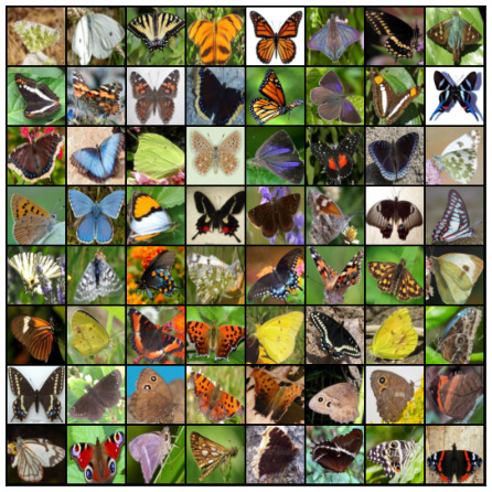
Figure 6.10 – The original butterfly images
Now, we can define the generator and discriminator module followed by the optimizer. The architecture is the same, so please feel free to repurpose the previous code. Once testing is done, you can train the model.
- Train the butterfly GAN model:
model = ButterflyGAN()
trainer = pl.Trainer( max_epochs=100, progress_bar_refresh_rate=25, gpus=1)#gpus=1,
trainer.fit(model, buttefly_train_dataloader)
In this code snippet we are training the Butterfly GAN model for 100 epochs
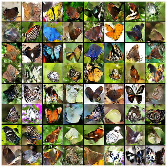
Figure 6.11 – Butterfly species generated from the GAN model
Important Note
Detecting GAN-generated fakes from real objects is a real challenge and an area of active research in Deep Learning community. It may be easy to detect fake butterflies here as some have weird colors, but not all. You may see some of the butterfly species as exotic Pacific butterflies, but make no mistake – all of them are totally fake. There are some tricks that you can use to identify fakes, such as a lack of symmetry or distorted colors. However, they are not foolproof, and more often than not, a human is deceived by a GAN-generated image.
GAN training challenges
A GAN model requires a lot of compute resources for training a model in order to get a good result, especially when a dataset is not very clean and representations in an image are not very easy to learn. In order to get a very clean output with sharp representations in our fake generated image, we need to pass a higher resolution image as input to our GAN model. However, the higher resolution means a lot more parameters are needed in the model, which in turn requires much more memory to train the model.
Here is an example scenario. We have trained our models using the image size of 64 pixels, but if we increase the image size to 128 pixels, then the number of parameters in the GAN model increases drastically from 15.9 M to 93.4 M. This, in turn, requires much more compute power to train the model, and with the limited resources in the Google Collab environment, you might get an error similar to this after 20–25 epochs:
RuntimeError: CUDA out of memory. Tried to allocate 64.00 MiB (GPU 0; 15.78 GiB total capacity; 13.94 GiB already allocated; 50.75 MiB free; 14.09 GiB reserved in total by PyTorch) If reserved memory is >> allocated memory try setting max_split_size_mb to avoid fragmentation. See documentation for Memory Management and PYTORCH_CUDA_ALLOC_CONF
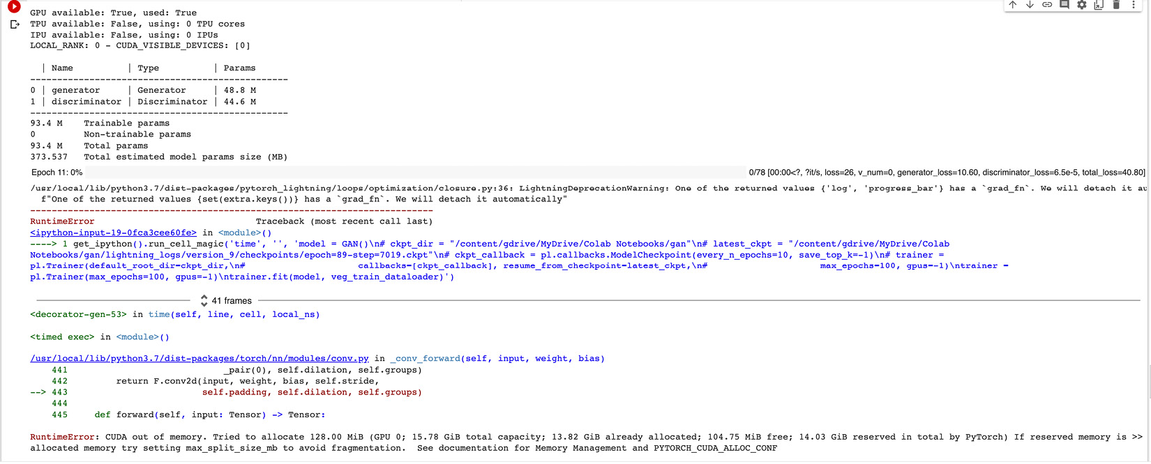
Figure 6.12 – A memory error on higher resolution images
There are some tricks to reduce memory utilization, such as reducing the batch size or gradient accumulation. However, there are limitations to these workarounds as well. For example, if you reduce the batch size to 64 from 128, the model will take much longer to learn representations in the image. You can observe this in the generated image when you reduce the batch size and train your model.
The model oscillates when the batch size is low because the gradients are averages for a fewer number of data instances. In such cases, the gradient accumulation technique can be used, which adds gradients of the parameters for n number of batches. This can be achieved by using the accumulate_grad_batches argument in the Trainer instance, as shown here:
# Accumulate gradients for 16 batches
trainer = Trainer(accumulate_grad_batches=16)
Therefore, you can combine these two parameters, the batch size and accumulate_grad_batches, to get a similar effective batch size for training higher resolution images, as shown here:
batch_size = 8
trainer = pl.Trainer(max_epochs=100, gpus=-1, accumulate_grad_batches=16)
This implies that the training will be done for an effective batch size of 128. However, the limitation is again the training time, so to train our model for much higher than 100 epochs in order to get a decent result using this technique while avoiding the out-of-memory error.
A lot of Deep Learning research areas are restricted by the amount of compute resources available to researchers. Most large tech companies (such as Google and Facebook) often come with new developments in the field, primarily due to their access to large servers and large datasets.
Creating images using DCGAN
A DCGAN is a direct extension of the GAN model discussed in the previous section, except that it explicitly uses the convolutional and convolutional-transpose layers in the discriminator and generator respectively. DCGAN was first proposed in a paper, Unsupervised Representation Learning with Deep Convolutional Generative Adversarial Networks, by Alec Radford, Luke Metz, and Soumith Chintala:
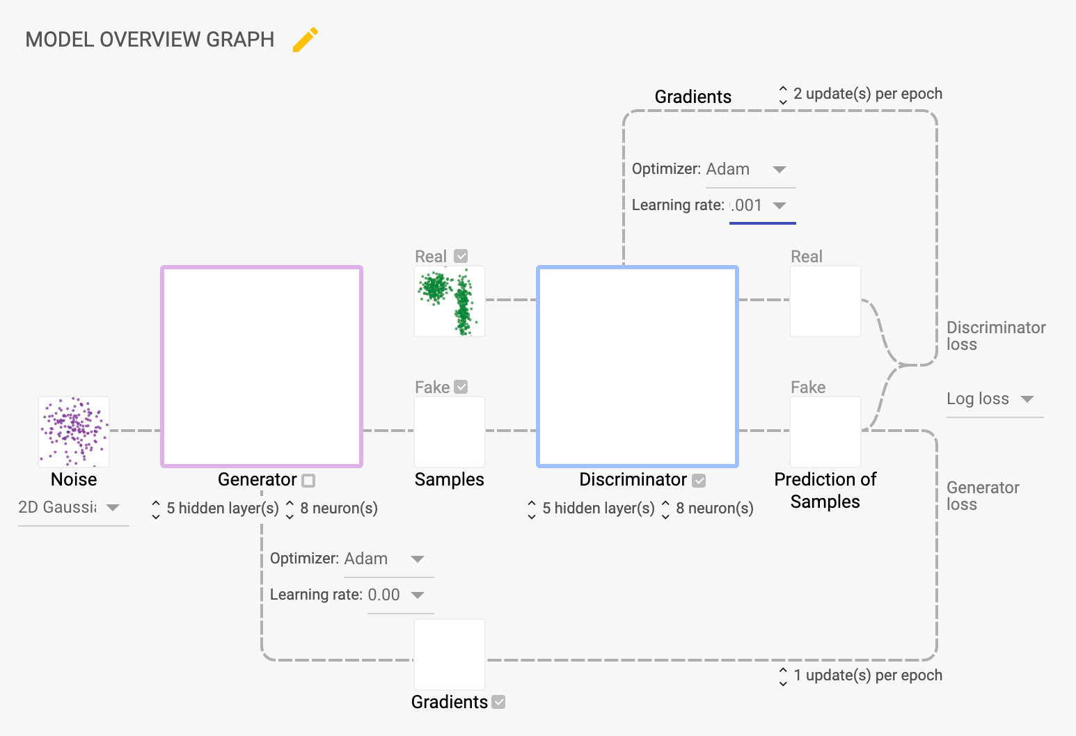
Figure 6.13 – A DCGAN architecture overview
The DCGAN architecture basically consists of 5 layers of convolution and 5 layers for transposed convolution. There is no fully connected layer in this architecture. We will also use a learning rate of 0.0002 for training the model.
We can also take a more in-depth look at the generator architecture of the DCGAN to see how it works:
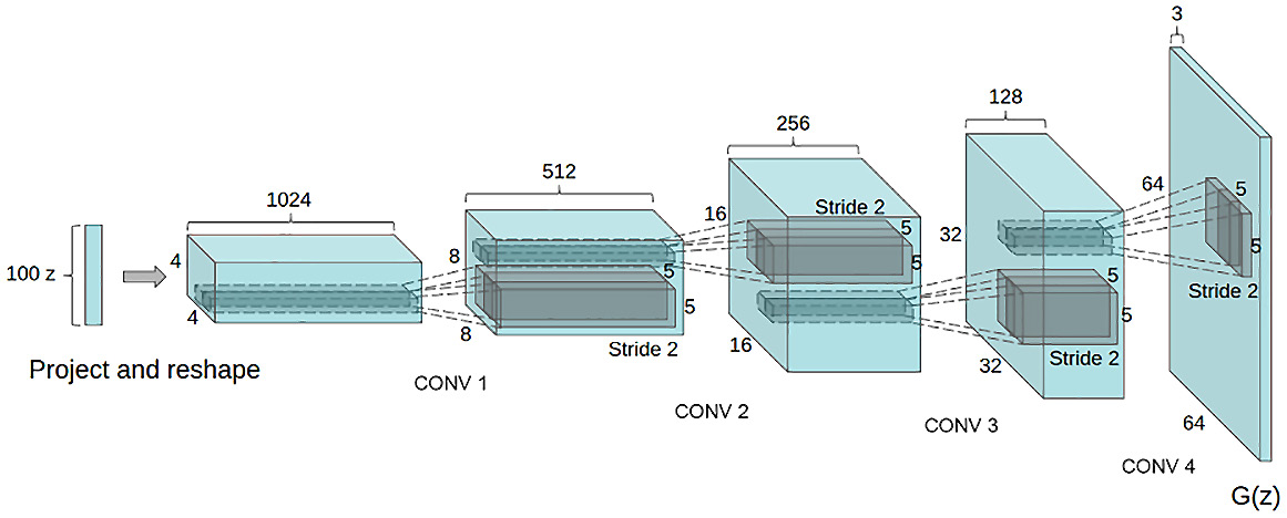
Figure 6.14 – The DCGAN generator architecture from the paper
It can be observed from the DCGAN generator architecture diagram that there are no fully connected or pooling layers used here. This is one of the architectural changes in the DCGAN model. The key advantage of DCGAN over GAN is its memory and compute efficiency. A tutorial for the DCGAN can be found on the PyTorch website.
We will use both the datasets (the food data and the butterfly data) on the same DCGAN model.
The code will consist of the following blocks:
- Defining inputs
- Loading data
- Weights initialization
- Discriminator model
- Generator model
- Optimizer
- Training
- Results
The code is very similar to the one we have just seen in the previous section. Please refer to the GitHub repository for this chapter for the full working code: https://github.com/PacktPublishing/Deep-Learning-with-PyTorch-Lightning/tree/main/Chapter06.
We trained the model for 100 epochs for both datasets, and the following is the loss we saw.
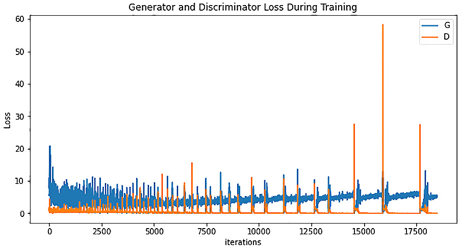
Figure 6.15 – Generator and discriminator loss during training of the DCGAN model
Based on the training, we get the following results for the food and butterfly datasets:
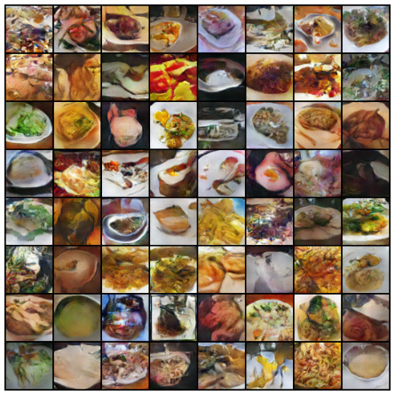
Figure 6.16 – Fake food images generated by the DCGAN model after 500 epochs
The following image shows the results for the butterfly dataset:

Figure 6.17 – Fake butterfly species generated by the DCGAN model after 500 epochs
As you will see, we get not just much better-quality results using DCGAN architecture but also with lesser epochs. The memory and compute requirements for the DCGAN were also lower than the vanilla GAN, and with the same amount of GPU, we could run the model for much longer. This is due to the inherent optimizations of the DCGAN, which makes it more efficient and effective.
Additional learning
- The first change that you can do to the model architecture is to change the number of convolutional and transposed convolutional layers. Most of the models use an eight-layer structure. You should change the preceding code to add more layers and compare the results.
- While we have used GAN and DCGAN architecture, you can also try other GAN architecture, such as BigGAN and StyleGAN.
- A GAN requires highly memory-intensive training. In order to reduce compute requirements, you can use pre-trained models. However, pre-trained models may only work with the original objects that they were trained for. As an example, you can generate new faces using a pre-trained StyleGAN model that was trained on a faces dataset. However, if there is no pre-trained model for butterflies (such as the dataset in this chapter), then it may not work well, and training from scratch may be the only option.
- Another option is to use a pre-trained model only for the discriminator. There are many papers that have used ImageNet pre-training for the discriminator only and got good results. You should try the same in this example as well.
- Lastly, go ahead and create anything new that you can dream of. GAN-created art is a new booming field. You can combine anything and generate anything. Who knows – your GAN art NFT may be auctioned at a high price one day!
Summary
GAN is a powerful method for generating not only images but also paintings, and even 3D objects (using newer variants of a GAN). We saw how, using a combination of discriminator and generator networks (each with five convolutional layers), we can start with random noise and generate an image that mimics real images. The play-off between the generator and discriminator keeps producing better images by minimizing the loss function and going through multiple iterations. The end result is fake pictures that never existed in real life.
It's a powerful method, and there are concerns about its ethical use. Fake images and objects can be used to defraud people; however, it also creates endless new opportunities. For example, imagine looking at a picture of fashion models while shopping for a new outfit. Instead of relying on endless image shoots, using a GAN (and DCGAN), you can generate realistic pictures of models with all body types, sizes, shapes, and colors, helping both companies and consumers. Fashion models are not the only example; imagine selling a home but having no furniture. Using a GAN, you can create realistic home furnishings – again, saving a lot of money for real estate developers. GANs are also a powerful source of data for augmentation and Deep Learning data generation purposes. Also, there are more possibilities for GANs that no one will have even thought of yet, and maybe you can come up with them by trying them out.
Next, we will continue our journey into generative modeling. Now that we have seen how to teach machines to generate images, we will try to teach machines how to write poems and generate text in the context of a given image. In the next chapter, we will explore Semi-Supervised Learning, where we will combine CNN and RNN architecture to generate human-like text, poems, or lyrics by making machines understand the context of what is inside an image.