Chapter 8: Self-Supervised Learning
Since the dawn of Machine Learning, the field has been neatly divided into two camps: supervised learning and unsupervised learning. In supervised learning, there should be a labeled dataset available, and if that is not the case, then the only option left is unsupervised learning. While unsupervised learning may sound great as it can work without labels, in practice, the applications of unsupervised methods such as clustering are quite limited. There is also no easy option to evaluate the accuracy of unsupervised methods or to deploy them.
The most practical Machine Learning applications tend to be supervised learning applications (for example, recognizing objects in images, predicting future stock prices or sales, or recommending the right movie to you on Netflix). The trade-off for supervised learning is the necessity for well-curated and high-quality trustworthy labels. Most datasets are not born with labels and getting such labels can be quite costly or at times downright impossible. One of the most popular Deep Learning datasets, ImageNet, consists of over 14 million images, with each label identifying an object in that image. As you may have guessed, the source images didn't come with those nice labels, so an army of 149,000 workers (mostly grad students) using Amazon's Mechanical Turk app spent over 19 months manually labeling each image. There are many datasets, such as medical X-ray images/CT scans for brain tumors, where doing this is simply impossible as it needs trained doctors, and there aren't many expert doctors available to label every image.
This begs the question, what if we can come up with a new method that can work without needing so many labels, such as unsupervised learning, but gives output that is as high-impact as supervised learning? That is exactly what Self-Supervised Learning promises to do.
Self-Supervised Learning is the latest paradigm in Machine Learning and is the most advanced frontier. While it has been theorized for a few years, it's only in the last year that it has been able to show results comparable to supervised learning and has become touted as the future of Machine Learning. The foundation of Self-Supervised Learning for images is that we can make machines learn a true representation even without labels. With a minuscule number of labels (as low as 1% of the dataset), we can achieve as good results as supervised models can. This unlocks the untapped potential in millions of datasets that are sitting unused due to the lack of high-quality labels.
In this chapter, we will get an introduction to Self-Supervised Learning and then go through one of the most widely used architectures in Self-Supervised Learning for image recognition known as contrastive representative learning. In this chapter, we will cover the following topics:
- Getting started with Self-Supervised Learning
- What is Contrastive learning?
- SimCLR architecture
- SimCLR contrastive learning model for image recognition
Technical requirements
In this chapter, we will be primarily using the following Python modules:
- NumPy (version 1.21.5)
- torch (version 1.10)
- torchvision (version 0.11.1)
- PyTorch Lightning (version 1.5.2)
Please check the correct version of the packages before running the code.
In order to make sure that these modules work together and not go out of sync, we have used the specifi c version of torch, torchvision, torchtext, torchaudio with PyTorch Lightning 1.5.2. You can also use the latest version of PyTorch Lightning and torch compatible with each other. More details can be found on the GitHub link:
https://github.com/PacktPublishing/Deep-Learning-with-PyTorch-Lightning.
!pip install torch==1.10.0 torchvision==0.11.1 torchtext==0.11.0 torchaudio==0.10.0 --quiet
!pip install pytorch-lightning==1.5.2 --quiet
Working examples for this chapter can be found at this GitHub link: https://github.com/PacktPublishing/Deep-Learning-with-PyTorch-Lightning/tree/main/Chapter08.
STL-10 source datasets can be found at https://cs.stanford.edu/~acoates/stl10/.
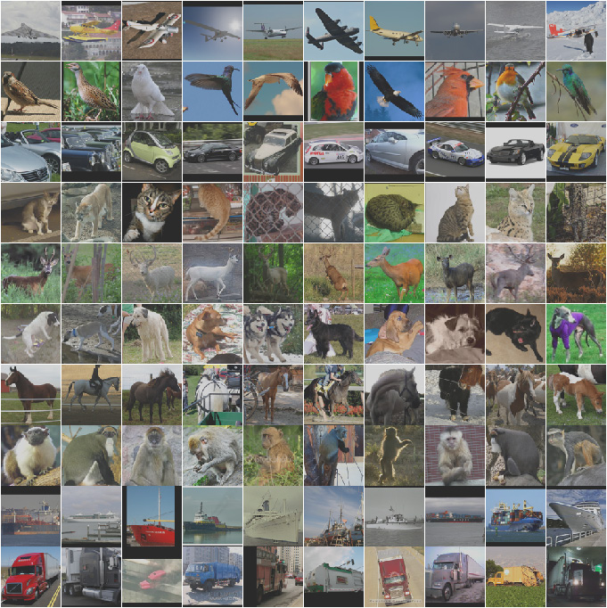
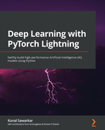
Figure 8.1 – A snapshot of STL-10 dataset
The STL-10 dataset is an image recognition dataset for developing Self-Supervised Learning algorithms. It is similar to CIFAR-10, but with a very important difference: each class has fewer labeled training examples than CIFAR-10, but a very large set of unlabeled examples is provided in order to learn image representations prior to supervised training.
Getting started with Self-Supervised Learning
The future of Machine Learning has been hotly contested given the spectacular success of Deep Learning methods such as CNN and RNN in recent years. While CNNs can do amazing things, such as image recognition, and RNNs can generate text, and other advanced NLP methods, such as the Transformer, can achieve marvelous results, all of them have serious limitations when compared to human intelligence. They don't compare very well to humans on tasks such as reasoning, deduction, and comprehension. Also, most notably, they require an enormous amount of well-labeled training data to learn even something as simple as image recognition.
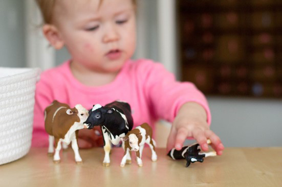
Figure 8.2 – A child learns to classify objects with very few labels
Unsurprisingly, that is not the way humans learn. A child does not need millions of labeled images as input before it can recognize objects. The incredible ability of the human brain to generate its own new labels based on a minuscule amount of initial information is unparalleled when compared to Machine Learning.
In order to expand the potential of AI, various other methods have been tried. The quest for achieving near-human intelligence performance led to two distinct methods, namely, Reinforcement learning and Self-supervised learning.
In Reinforcement Learning, the focus is on constructing a game-like environment and making a machine learn how to navigate through the environment without explicit directions. Each system is configured to maximize the reward function and, slowly, agents learn by making mistakes in each game event and then minimize those mistakes in the next event. Doing so requires a model to be trained for millions of cycles, which sometimes translates to thousands of years of human time. While this method has beaten humans at very difficult games such as Go and set a new benchmark for machine intelligence, clearly this is not how humans learn. We don't practice a game for thousands of years before being able to play it. Also, so many trials make it too slow to learn for any practical industrial applications.
In Self-Supervised Learning, however, the focus is on making the machine learn a bit like a human by trying to create its own labels and continue to learn adaptively. The term Self-Supervised Learning is the brainchild of Yann LeCun, one of the Turing Award recipients (the equivalent of the Nobel Prize for computing) for making a foundational contribution to Deep Learning. He also laid the groundwork for Self-Supervised Learning as well and conducted a lot of research using energy modeling methods.
Figure 8.3 – Future belongs to "Self-Supervised Learning"
Most notably, Yann LeCun argued that the future of AI will neither be supervised nor reinforced, but will be self-supervised! This is arguably the most important area, with the potential to disrupt the way we know Machine Learning.
So, what does it mean to be Self-Supervised?
The core concept is that we can learn in multiple dimensions of data. In supervised learning, we have data (x) and labels (y), and we can do a lot of things, such as prediction, classification, and object detection, whereas, in unsupervised learning, we only have data (x), and we can only do clustering types of models. In unsupervised learning, we have the advantage that we don't need costly labels, but the kinds of models we can build are limited. What if we start in an unsupervised manner (with only x and then somehow generate labels (y) for the dataset) and then move on to supervised learning?
In other words, what if we can make the machine learn to generate its own labels as it goes along? Currently, say I have an image dataset such as CIFAR-10 that consists of 10 classes of images (classes such as bird, airplane, dog, and cat) spread over 65,000 labels. This is what machine needs to learn to recognize those 10 classes. What if, instead of supplying 65,000 labels, as we did for this dataset, I supply only 10 labels (one for each class) and then the machine finds images similar to those classes and adds labels to them? If we can do that, then the machine is self-supervising its learning process, and it will be able to scale to solve previously unsolved problems.
What I have provided here is a rather simplistic definition of Self-Supervised Learning. Yann LeCun defined Self-Supervised Learning mostly in the context of Energy Modelling as a model that can learn not just forward from backward but in any direction. Energy modeling is an area of active research in the Deep Learning community. Ideas such as Concept Learning, whereby a model learns a concept of image and label together, may be revolutionary in the future. Also, there is one Self-Supervised Learning application you may have already heard of. NLP models such as GPT3 and Transformers have been trained with no labels and still can be fine-tuned or adjusted easily for any task. You can appreciate that language is a unidimensional data structure as data normally flows in one direction (backward to forward, as we read English from left to right), and so it's easy to learn structure without any labels being associated with it.
In other areas, such as images or structured data, learning without labels or with a very limited number of labels has proven to be challenging. One area that we will focus on in this chapter that has got very interesting results in recent months is contrastive learning, in which we can find similar images from dissimilar images without having any labels associated with them.
Important Note
To learn more about energy modeling, it is advisable to go through lectures focusing on them. Refer to the online lecture entitled "A Tutorial on Energy-Based Learning," by Yann LeCun: https://training.incf.org/lesson/energy-based-models-i.
What is Contrastive Learning?
The idea of understanding an image is to get an image of a particular kind (say a dog) and then we can recognize all other dogs by reasoning that they share the same representation or structure. For example, if you show a child who is not yet able to talk or understand language (say, less than 2 years old) a picture of a dog (or a real dog for that matter) and then give them a pack of cards with a collection of animals, which includes dogs, cats, elephants, and birds, and ask the child which picture is similar to the first one, it is most likely that the child could easily pick the card with a dog on it. And the child would be able to do so even without you explaining that this picture equals "dog" (in other words, without supplying any new labels).
You could say that a child learned to recognize all dogs in a single instance and with a single label! Wouldn't it be awesome if a machine could do that as well? That is exactly what contrastive learning is!
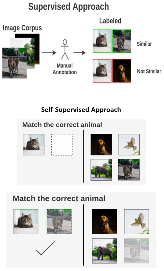
Figure 8.4 – How contrastive learning differs from supervised learning (Source: https://amitness.com/2020/03/illustrated-simclr/)
What is happening here is a form of representation learning. In fact, the full name of this method is contrastive representation learning. The child has understood that a dog has a certain type of representation (a tail, four legs, eyes, and so on) and then is able to find similar representations. Astonishingly, the human brain does this with a surprisingly minuscule amount of data (even a single image is enough to teach someone a new object). In fact, child development experts have theorized that when the child is barely a few months old, it begins to recognize its mother and father and other familiar objects purely by creating loose representations (like silhouettes). This is one of the key development stages when it begins to accept new visual data and start the process of recognition and classification. This visual ability, which makes us see as opposed to just look at objects, is very crucial in our intellectual development. Similarly, the ability to make a machine learn how images differ from each other without passing any labels is an important milestone in the development of AI.
There have been various proposed architectures for contrastive learning that have had spectacular results. Some popular ones are SimCLR, CPC, YADIM, and NOLO. In this chapter, we will see the architecture that is fast becoming a de facto standard for contrastive learning – SimCLR.
SimCLR architecture
SimCLR stands for Simple Contrastive Learning Architecture. This architecture is based on the paper "A Simple Framework for Contrastive Learning of Visual Representations", published by Geoffrey Hinton and Google Team. Geoffrey Hinton (just like Yann LeCun) is a co-recipient of the Turing Award for his work on Deep Learning. There are SimCLR and SimCLR2 versions. SimCLR2 is a larger and denser network than SimCLR. At the time of writing, SimCLR2 was the best architecture update available, but don't be surprised if there is a SimCLR3 soon that is even denser and better than the previous one.
The architecture has shown in relation to the ImageNet dataset that we can achieve 93% accuracy with just 1% of labels. This is a truly remarkable result considering that it took over 2 years and a great deal of effort from over 140,000 labelers (mostly graduate students) on Mechanical Turk to label ImageNet by hand. It was a massive undertaking carried out on a global scale. Apart from the sheer amount of time it took to label that dataset, it also became clear that without the backing of big companies such as Google, such an endeavor is difficult. It may come as no surprise to you that many datasets are lying unused simply because they are not properly labeled. If we can achieve comparable results with just 1% of labels, it would open the previously unopened doors in what Deep Learning can do!
How does SimCLR work?
Let's have a quick overview of how SimCLR works. We urge you to read the full paper mentioned in the previous section for more details.
The idea behind contrastive learning is that we want to group similar images while differentiating them at the same time from dissimilar images. This process takes place on an unlabeled set of images.
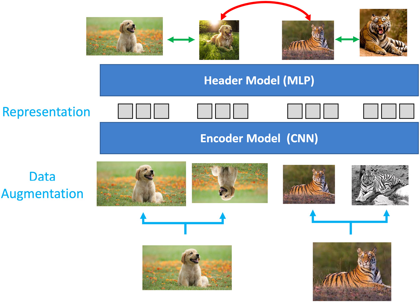
Figure 8.5 – How SimCLR works (Note: the architecture is executed from the bottom up)
The architecture consists of the following building blocks:
- As a first step, data augmentation is performed on the group of random images. Various data augmentation tasks are performed. Some of them are standard ones, such as rotating the images, cropping them, and changing the color by making them grayscale. Other more complex data augmentation tasks, such as Gaussian Blur, are also performed. You will find that the more complex or sophisticated the augmentation transforms, the more useful it is for the model.
This data augmentation step is very important since we want to make the model learn the true representation reliably and consistently. Another, and rather important, reason is that we don't have labels in the dataset. So, we have no way of knowing which images are actually similar to each other and which are dissimilar. And thus, having various augmented images from a single image creates a "true" set of similar images for the model that we can be apriori sure of.
- The next step is then to create a batch of images that contains similar and dissimilar images. As an analogy, this can be thought of as a batch that has some positive ions and some negative ions, and we want to isolate them by moving a magical magnet over them (SimCLR).
- This process is followed by an encoder that is nothing but a CNN architecture. ResNet architectures such as ResNet-18 or ResNet-50 are most commonly used for this operation. However, we strip away the last layer and use the output after the last average pool layer. This encoder helps us learn the image representations.
- This is followed by the header module (also known as projection head), which is a Multi-Layer Perceptron (MLP) model. This is used to map contrastive loss to the space where the representations from the previous step are applied. Our MLP can be a single hidden layer neural network (as in SimCLR) or a 3-layer network (as it is in SimCLR2). You can even experiment with larger neural networks. This step is used to balance alignment (keeping similar images together) and uniformity (preserve the maximum amount of information).
- The key in this step is the contrastive loss function that is used for contrastive prediction. Its job is to identify other positive images in a dataset. The specialized loss function used for this is NT-Xent (the normalized temperature-scaled, cross-entropy loss). This loss function helps us measure how the system is learning in subsequent epochs.
These steps describe the SimCLR architecture and, as you may have noted, it works purely on unlabeled images. The magic of SimCLR is realized when you fine-tune it for a downstream task such as image classification. This architecture can learn features for you, and then you can use those features for any task.

Figure 8.6 – Semi-supervised approach for finding relevant images
The task could be to find whether images in your dataset are relevant to your objective. Imagine you want to save tigers by creating an image recognition model for tigers and you only want tiger images. Any camera traps may include other animals (and even unrelated objects). But not all your images will be labeled. You can build a Semi-Supervised Learning model by using SimCLR architecture followed by a supervised classifier for whatever small number of labels you have and get your data cleaned. It can also be thought of as transfer learning by transferring the weights learned through the representation learning of the SimCLR model to subsequent classification tasks.
Another more basic task could be to classify images by supplying very few labels and features from the SimCLR architecture. The question that may occur to you is "just how little?" Experiments have shown that for a downstream task that is just 10% or even 1% labeled, we can get nearly 95% accuracy.
SimCLR model for image recognition
We have seen that SimCLR can do the following:
- Learn feature representations (unit hypersphere) by grouping similar images together and pushing dissimilar images apart.
- Balance alignment (keeping similar images together) and uniformity (preserving the maximum information).
- Learn on unlabeled training data.
The primary challenge is to use the unlabeled data (that comes from a similar but different distribution from the labeled data) to build a useful prior, which is then used to generate labels for the unlabeled set. Let's look at the architecture we will implement in this section.

Figure 8.7 – SimCLR architecture implementation
We will use the ResNet-50 as the Encoder, followed by a three-layer MLP as the projection head. We will then use logistic regression, or MLP, as the supervised classifier to measure the accuracy.
The SimCLR architecture involves the following steps, which we implement in code:
- Collecting the dataset
- Setting up data augmentation
- Loading the dataset
- Configuring training
- Training the SimCLR model
- Evaluating the performance
Collecting the dataset
We will use the STL-10 dataset from https://cs.stanford.edu/~acoates/stl10/.
As described on the dataset web page, the STL-10 dataset is an image recognition dataset for developing Self-Supervised Learning algorithms. It consists of the following:
- 10 classes: airplane, bird, car, cat, deer, dog, horse, monkey, ship, and truck.
- Images are 96x96 pixels and in color.
- 500 training images (10 pre-defined folds) and 800 test images per class.
- 100,000 unlabeled images for unsupervised learning. These examples are extracted from a similar but broader distribution of images. For instance, it contains other types of animals (bears, rabbits, and so on) and vehicles (trains, buses, and so on) in addition to the ones in the labeled set.
The binary files are split into data and label files with suffixes train_X.bin, train_y.bin, test_X.bin, and test_y.bin.
You can download the binary files directly from http://ai.stanford.edu/~acoates/stl10/stl10_binary.tar.gz and put them in your data folder. Or, to work on a cloud instance, execute the full Python code available at https://github.com/mttk/STL10. The STL-10 dataset is also available in the torchvision module under https://pytorch.org/vision/stable/datasets.html#stl10 and can also be directly imported into the notebook.
Since the STL-10 dataset is scraped from ImageNet, any pre-trained model on ImageNet can be used to accelerate training by using pre-trained weights.
The SimCLR model depends on three packages: pytorch, torchvision, and pytorch_lightning. As a first step, please install and import these packages into your notebook. Once the packages are installed, we will go about importing them:
import os
import urllib.request
from copy import deepcopy
from urllib.error import HTTPError
import matplotlib
import matplotlib.pyplot as plt
import pytorch_lightning as pl
import seaborn as sns
import torch
import torch.nn as nn
import torch.nn.functional as F
import torch.optim as optim
import torch.utils.data as DataLoader
from IPython.display import set_matplotlib_formats
from pytorch_lightning.callbacks import LearningRateMonitor, ModelCheckpoint
from pytorch_lightning.callbacks import ModelCheckpoint
from pytorch_lightning.callbacks import Callback
import torchvision
from torchvision import transforms
import torchvision.models as models
from torchvision import datasets
from torchvision.datasets import STL10
from tqdm.notebook import tqdm
from torch.optim import Adam
import numpy as np
from torch.optim.lr_scheduler import OneCycleLR
import zipfile
from PIL import Image
import cv2
After the necessary packages are imported, we have to collect the images in STL-10 format. We can download the data from the Stanford repository into our local data path to be used for further processing. You should add the path of the folder where you have downloaded the STL-10 files.
Setting up data augmentation
The first step that we need to do is to create a data augmentation module. This is an extremally important step in SimCLR architecture, and the final result is greatly affected by the richness of the transformations undertaken in this step.
Important Note
PyTorch Lightning also includes various SimCLR transforms out of the box using Bolts. We are, however, manually defining it here. You can also refer to out-of-the-box transforms here for various approaches: https://pytorch-lightning-bolts.readthedocs.io/en/latest/transforms.html#simclr-transforms. Please be careful about your PyTorch Lightning version and the torch version to use them.
Our goal is to create a positive set that can easily be achieved by creating multiple copies of a given image and applying various augmentation transformations to it. As a first step, we can create as many image copies as we want:
class DataAugTransform:
def __init__(self, base_transforms, n_views=4):
self.base_transforms = base_transforms
self.n_views = n_views
def __call__(self, x):
return [self.base_transforms(x) for i in range(self.n_views)]
In the preceding code snippet, we are creating four copies of the same image.
We will now go ahead and apply four key transforms to the images. As per the original paper and further research, the cropping and resizing of images are crucial transforms and help the model to learn better:
augmentation_transforms = transforms.Compose(
[
transforms.RandomHorizontalFlip(),
transforms.RandomResizedCrop(size=96),
transforms.RandomApply([transforms.ColorJitter(brightness=0.8, contrast=0.8, saturation=0.8, hue=0.1)], p=0.8),
transforms.RandomGrayscale(p=0.2),
transforms.ToTensor(),
transforms.Normalize((0.5,), (0.5,)),
]
)
In the preceding code snippet, we augment the image and perform the following transforms:
- Random resize and crop
- Random horizontal flip
- Random color jitter
- Random grayscale
Please note that the data augmentation step can take a considerable amount of time to finish for a reasonably large dataset.
Important Note
One of the heavier transforms that is mentioned in the SimCLR paper but not performed here is a Gaussian Blur. It blurs images by adding noise using the Gaussian function by giving more weight to the center part of the image than other parts. The final average effect is to reduce the detail of the image. You can optionally perform a Gaussian Blur transform as well on the STL-10 images. In the new version of torchvision, you can use the following option to perform it: #transforms.GaussianBlur(kernel_size=9).
Loading the dataset
Now, we will define the path to download the dataset and collect it:
DATASET_PATH = os.environ.get("PATH_DATASETS", "bookdata/")
CHECKPOINT_PATH = os.environ.get("PATH_CHECKPOINT", "booksaved_models/")
In the preceding code snippet, we defined the dataset and checkpoint path.
We will now apply the transforms to the STL-10 dataset and create two views of it:
unlabeled_data = STL10(
root=DATASET_PATH,
split="unlabeled",
download=True,
transform=DataAugTransform(augmentation_transforms, n_views=2),
)
train_data_contrast = STL10(
root=DATASET_PATH,
split="train",
download=True,
transform=DataAugTransform(augmentation_transforms, n_views=2),
)
It then transforms into a torch tensor for model training by applying the data augmentation process. We can verify the output of the preceding process by visualizing some of the images:
pl.seed_everything(96)
NUM_IMAGES = 20
imgs = torch.stack([img for idx in range(NUM_IMAGES) for img in unlabeled_data[idx][0]], dim=0)
img_grid = torchvision.utils.make_grid(imgs, nrow=8, normalize=True, pad_value=0.9)
img_grid = img_grid.permute(1, 2, 0)
plt.figure(figsize=(20, 10))
plt.imshow(img_grid)
plt.axis("off")
plt.show()
In the preceding code snippet, we print the original image along with the augmented one. This should show the following result:

Figure 8.8 – STL-10 augmented images
As you can see, various image transforms have been applied successfully. The multiple copies of the same image will serve as a positive set of pairs for the model to learn.
Training configuration
Now we will set up the configuration of the model training, which includes hyperparameters, the loss function, and the encoder.
Setting hyperparameters
We will use the YAML file to pass on various hyperparameters to our model training. Having a YAML file makes it easy to create various experiments:
weight_decay: 10e-6
out_dim: 256
dataset:
s: 1
input_shape: (96,96,3)
num_workers: 4
optimizer:
lr: 0.0001
loss:
temperature: 0.05
use_cosine_similarity: True
lr_schedule:
max_lr: .1
total_steps: 1500
model:
out_dim: 128
base_model: "resnet50"
'''
config = yaml.full_load(config)
The preceding code snippet will load the YAML file and set the following hyperparameters:
- batch_size: The batch size to use for training.
- Epochs: The number of epochs to run the training for.
- out_dim: The output dimensions of the embedding layer.
- s: The brightness, contrast, saturation, and hue level of the color jitter transformation.
- input_shape: The input shape to the model after the final image transformation. All raw images will be resized to this shape (H, W, color channels).
- num_workers: The number of workers to use for the data loader. It can increase training speed by pre-fetching and processing data.
- lr: The initial learning rate to use for training.
- temperature: The temperature-tuning parameter to smooth the probabilities of the loss function.
- use_cosine_similarity: A Boolean indicator of whether to use cosine similarity in the loss function.
- max_lr: The maximum learning rate for the 1cycle learning rate scheduler.
- total_steps: The total number of training steps for the 1cycle learning rate scheduler.
Important Note on Batch Size
The batch size plays a very important role in contrastive learning models. In SimCLR, it has been observed that having a large batch size is associated with better results. However, a large batch size also requires much more compute in the form of GPU.
Defining the loss function
The purpose of the loss function is to help distinguish between positive and negative pairs. The original paper describes the NTXent loss function.
We will now go ahead and implement this loss function in the code:
import yaml # Handles config file loading
# Load config file
config = '''
batch_size: 128
epochs: 100
class NTXentLoss(torch.nn.Module):
def __init__(self, device, batch_size, temperature, use_cosine_similarity):
super(NTXentLoss, self).__init__()
self.batch_size = batch_size
self.temperature = temperature
self.device = device
self.softmax = torch.nn.Softmax(dim=-1)
self.mask_samples_from_same_repr = self._get_correlated_mask().type(torch.bool)
self.similarity_function = self._get_similarity_function(use_cosine_similarity)
self.criterion = torch.nn.CrossEntropyLoss(reduction="sum").cuda()
def _get_similarity_function(self, use_cosine_similarity):
if use_cosine_similarity:
self._cosine_similarity = torch.nn.CosineSimilarity(dim=-1)
return self._cosine_simililarity
else:
return self._dot_simililarity
def _get_correlated_mask(self):
diag = np.eye(2 * self.batch_size)
l1 = np.eye((2 * self.batch_size), 2 * self.batch_size, k=-self.batch_size)
l2 = np.eye((2 * self.batch_size), 2 * self.batch_size, k=self.batch_size)
mask = torch.from_numpy((diag + l1 + l2))
mask = (1 - mask).type(torch.bool)
return mask.to(self.device)
@staticmethod
def _dot_simililarity(x, y):
v = torch.tensordot(x.unsqueeze(1), y.T.unsqueeze(0), dims=2)
return v
def _cosine_simililarity(self, x, y):
v = self._cosine_similarity(x.unsqueeze(1), y.unsqueeze(0))
return v
def forward(self, zis, zjs):
representations = torch.cat([zjs, zis], dim=0)
similarity_matrix = self.similarity_function(representations, representations)
# filter out the scores from the positive samples
l_pos = torch.diag(similarity_matrix, self.batch_size)
r_pos = torch.diag(similarity_matrix, -self.batch_size)
positives = torch.cat([l_pos, r_pos]).view(2 * self.batch_size, 1)
negatives = similarity_matrix[self.mask_samples_from_same_repr].view(2 * self.batch_size, -1)
logits = torch.cat((positives, negatives), dim=1)
logits /= self.temperature
labels = torch.zeros(2 * self.batch_size).to(self.device).long()
loss = self.criterion(logits, labels)
return loss / (2 * self.batch_size)
In the preceding code snippet, we implemented the NTXtent loss function, which will measure the loss for the positive pairs. Do remember that the task of the model is to minimize the loss between positive pairs and, hence, this loss function.
Defining the encoder
We can use any encoder architecture (such as VGGNet, or AlexNet, or ResNet, and so on). Since the original paper has ResNet, we will also use ResNet as our encoder:
class ResNetSimCLR(nn.Module):
def __init__(self, base_model, out_dim, freeze=True):
super(ResNetSimCLR, self).__init__()
# Number of input features into the last linear layer
num_ftrs = base_model.fc.in_features
# Remove last layer of resnet
self.features = nn.Sequential(*list(base_model.children())[:-1])
if freeze:
self._freeze()
In the preceding code block, we have removed the last softmax layer of ResNet and passed on the feature to the next module. We can follow this up with a header projection code block using an MLP model. While SimCLR1 has a single-layer MLP, SimCLR2 has a 3-layer MLP, which is what we will use here. Others have also got good results with a 2-layer MLP model. (Please note that this code is part of the same class as above:)
# header projection MLP - for SimCLR
self.l1 = nn.Linear(num_ftrs, 2*num_ftrs)
self.l2_bn = nn.BatchNorm1d(2*num_ftrs)
self.l2 = nn.Linear(2*num_ftrs, num_ftrs)
self.l3_bn = nn.BatchNorm1d(num_ftrs)
self.l3 = nn.Linear(num_ftrs, out_dim)
def _freeze(self):
num_layers = len(list(self.features.children())) # 9 layers, freeze all but last 2
current_layer = 1
for child in list(self.features.children()):
if current_layer > num_layers-2:
for param in child.parameters():
param.requires_grad = True
else:
for param in child.parameters():
param.requires_grad = False
current_layer += 1
def forward(self, x):
h = self.features(x)
h = h.squeeze()
if len(h.shape) == 1:
h = h.unsqueeze(0)
x_l1 = self.l1(h)
x = self.l2_bn(x_l1)
x = F.selu(x)
x = self.l2(x)
x = self.l3_bn(x)
x = F.selu(x)
x = self.l3(x)
return h, x_l1, x
In the preceding code snippet, we have defined the convolutional layers for the ResNet and then frozen the last layer and used that feature as an input to a projection head model, which is a 3-layer MLP.
Now, we can extract the features from either the last layer of ResNet or from the last layer of the 3-layer MLP model and use it as a true representation of the images that the model has learned.
Important Note
While ResNet with SimCLR will be available as a pre-trained model for STL-10, if you are trying SimCLR architecture for another dataset, this code will be useful for training it from scratch.
SimCLR pipeline
Now that we have put in place all the building blocks for the SimCLR architecture, we can finally construct the SimCLR pipeline:
class simCLR(pl.LightningModule):
def __init__(self, model, config, optimizer=Adam, loss=NTXentLoss):
super(simCLR, self).__init__()
self.config = config
# Optimizer
self.optimizer = optimizer
# Model
self.model = model
# Loss
self.loss = loss(self.config['batch_size'], **self.config['loss'])
# Prediction/inference
def forward(self, x):
return self.model(x)
# Sets up optimizer
def configure_optimizers(self):
optimizer = self.optimizer(self.parameters(), **self.config['optimizer'])
scheduler = OneCycleLR(optimizer, **self.config["lr_schedule"])
return [optimizer], [scheduler]
In the preceding code snippet, we have used the config file (dictionary) to pass on parameters to each module: optimizer, loss, and lr_schedule. We are using the Adam optimizer and calling the NTXtent loss function that we constructed previously.
Now we can add training and validation loops to the same class:
# Training loops
def training_step(self, batch, batch_idx):
x, y = batch
xis, xjs = x
ris, _, zis = self(xis)
rjs, _, zjs = self(xjs)
zis = F.normalize(zis, dim=1)
zjs = F.normalize(zjs, dim=1)
loss = self.loss(zis, zjs)
return loss
# Validation step
def validation_step(self, batch, batch_idx):
x, y = batch
xis, xjs = x
ris, _, zis = self(xis)
rjs, _, zjs = self(xjs)
zis = F.normalize(zis, dim=1)
zjs = F.normalize(zjs, dim=1)
loss = self.loss(zis, zjs)
self.log('val_loss', loss)
return loss
def test_step(self, batch, batch_idx):
loss = None
return loss
def _get_model_checkpoint():
return ModelCheckpoint(
filepath=os.path.join(os.getcwd(),"checkpoints","best_val_models"),
save_top_k = 3,
monitor="val_loss"
)
In the preceding code snippet, we have created a model class that takes the following inputs:
- Hyperparameters from the config file
- NTXtent as a loss function
- Adam as the optimizer
- An encoder as a model (can be changed to any model other than ResNet if desired)
We further define the training and validation loops to calculate the loss and finally save the model checkpoint.
Important Note
It is advisable that you should construct a callback class, which will save the model checkpoint and resume the model training from the saved checkpoint. It can also be useful for passing preconfigured weights of the encoder. Please refer to GitHub or Chapter 10 for more details.
Model training
Now that we have defined the model configuration, we can move on to model training.
We will first use a data loader to load the data:
train_loader = DataLoader.DataLoader(
unlabeled_data,
batch_size=128,
shuffle=True,
drop_last=True,
pin_memory=True,
num_workers=NUM_WORKERS,
)
val_loader = DataLoader.DataLoader(
train_data_contrast,
batch_size=128,
shuffle=False,
drop_last=True,
pin_memory=True,
num_workers=NUM_WORKERS,
)
We will use the ResNet-50 architecture as the encoder. You can play with other ResNet architectures, such as ResNet-18 or ResNet-152, and compare the results:
resnet = models.resnet50(pretrained=True)
simclr_resnet = ResNetSimCLR(base_model=resnet, out_dim=config['out_dim'])
In the preceding code snippet, we import the ResNet CNN model architecture and use pretrained=True to use the pre-trained weights of the model to speed up the training. Since the PyTorch ResNet model is trained on the ImageNet dataset and our STL-10 dataset is also scraped from ImageNet, using the pre-trained weights is a reasonable choice.
We will now initiate the training process:
model = simCLR(config=config, model=simclr_resnet)
trainer = pl.Trainer()
You should see the following information, depending on the hardware you are using:
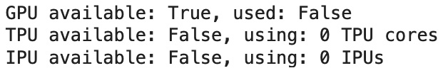
Figure 8.9 – GPU available for model training
In the preceding code snippet, we create the SimCLR model from the architecture mentioned and use the trainer to fit the model by passing the dataset from the data loader:
trainer.fit(model, train_loader, val_loader)
This should show you the following initiation of the training process:
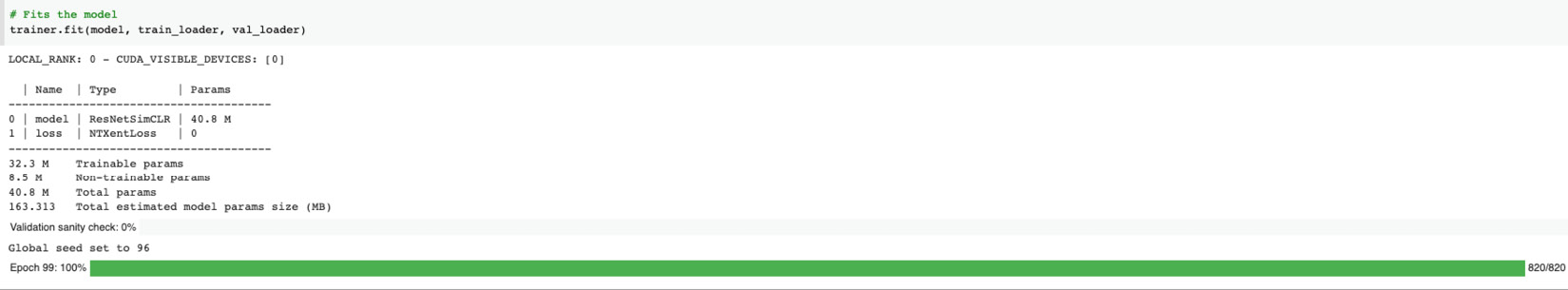
Figure 8.10 – SimCLR training process
The sharp-eyed among you may have noticed that it is using the NTXent loss function.
Important Note
Depending on the hardware you have access to, you can use various options in the PyTorch Lightning framework to speed up the training process. As shown in Chapter 7, Semi-Supervised Learning, if you are using a GPU, then you can use the gpu=-1 option and also enable 16-bit precision for mixed-mode precision training. Refer to Chapter 10 for more details on options for scaling up the training process.
Once the model is trained, you can save the model weight
torch.save(model.state_dict(), 'weights_only.pth')
torch.save(model, 'entire_model.pth')
This will save the model weights as `weights_only.pth and the entire model as `entire_model.pth'
Model evaluation
While the SimCLR model architecture will learn the representation of the unlabeled images, we still need a method to measure how well it learned those representations. In order to do this, we use a supervised classifier that has some labeled images (from the original STL-10 dataset), and then we use the features learned in the SimCLR model to apply the feature map for images learned via representation learning and then compare the results.
Model evaluation therefore consists of three steps:
- Extracting the features from the SimCLR model
- Defining a classifier
- Predicting accuracy
We can try to compare the results by passing a very limited number of labels, such as 500 or 5,000 (or 1 to 10%), and then also compare the results with the supervised classifier, which has been trained with 100% of the labels. This will help us to compare how well our self-supervised model was able to learn representations from unlabeled images.
Feature extraction from the SimCLR model
We first need to extract the features learned from the model. To do so, we load the model
def _load_resnet_model(checkpoints_folder):
model = torch.load('entire_model.pth')
model.eval()
state_dict = torch.load(os.path.join(checkpoints_folder, 'weights_only.pth'), map_location=torch.device(device))
model.load_state_dict(state_dict)
model = model.to(device)
return model
This code snippet will load the pre-trained SimCLR model weights from weights_only.pth and the entire model from entire_model.pth.
Now we can use the data loader to instantiate the training and test split:
def get_stl10_data_loaders(download, shuffle=False, batch_size=128):
train_dataset = datasets.STL10('./data', split='train',
download=download,
transform=transforms.
ToTensor())
train_loader = DataLoader.DataLoader(train_dataset, batch_size=batch_size,num_workers=4, drop_last=False,
shuffle=shuffle)
test_dataset = datasets.STL10('./data', split='test',
download=download,
transform=transforms.
ToTensor())
test_loader = DataLoader.DataLoader(test_dataset, batch_size=batch_size,
num_workers=4, drop_last=False,
shuffle=shuffle)
return train_loader, test_loader
In this code snippet, the training and test datasets are instantiated.
We can now define the feature extractor class:
class ResNetFeatureExtractor(object):
def __init__(self, checkpoints_folder):
self.checkpoints_folder = checkpoints_folder
self.model = _load_resnet_model(checkpoints_folder)
def _inference(self, loader):
feature_vector = []
labels_vector = []
for batch_x, batch_y in loader:
batch_x = batch_x.to(device)
labels_vector.extend(batch_y)
features, _ = self.model(batch_x)
feature_vector.extend(features.cpu().detach().numpy())
feature_vector = np.array(feature_vector)
labels_vector = np.array(labels_vector)
print("Features shape {}".format(feature_vector.shape))
return feature_vector, labels_vector
def get_resnet_features(self):
train_loader, test_loader = get_stl10_data_loaders(download=True)
X_train_feature, y_train = self._inference(train_loader)
X_test_feature, y_test = self._inference(test_loader)
return X_train_feature, y_train, X_test_feature, y_test
In the preceding code snippet, we get the features extracted from the ResNet model we have trained. We can validate this by printing the shapes of the file:
checkpoints_folder = ''
resnet_feature_extractor = ResNetFeatureExtractor(checkpoints_folder)
X_train_feature, y_train, X_test_feature, y_test = resnet_feature_extractor.get_resnet_features()
You should see the following output, which shows the shapes of the training and test files:
Files already downloaded and verified
Files already downloaded and verified
Features shape (5000, 2048)
Features shape (8000, 2048)
Now that we are ready, we can define the supervised classifier to train the supervised model on top of the Self-Supervised features.
Supervised classifier
We can use any supervised classifier for this task, such as MLP or logistic regression. In this module, we will choose logistic regression. In this section, we are using the scikit-learn module to implement logistic regression.
We start by defining the LogisticRegression class:
import torch.nn as nn
class LogisticRegression(nn.Module):
def __init__(self, n_features, n_classes):
super(LogisticRegression, self).__init__()
self.model = nn.Linear(n_features, n_classes)
def forward(self, x):
return self.model(x)
The preceding step will instantiate the class. This is followed by defining the configuration for the logistic regression model:
class LogiticRegressionEvaluator(object):
def __init__(self, n_features, n_classes):
self.log_regression = LogisticRegression(n_features, n_classes).to(device)
self.scaler = preprocessing.StandardScaler()
def _normalize_dataset(self, X_train, X_test):
print("Standard Scaling Normalizer")
self.scaler.fit(X_train)
X_train = self.scaler.transform(X_train)
X_test = self.scaler.transform(X_test)
return X_train, X_test
def _sample_weight_decay():
weight_decay = np.logspace(-7, 7, num=75, base=10.0)
weight_decay = np.random.choice(weight_decay)
print("Sampled weight decay:", weight_decay)
return weight_decay
def eval(self, test_loader):
correct = 0
total = 0
with torch.no_grad():
self.log_regression.eval()
for batch_x, batch_y in test_loader:
batch_x, batch_y = batch_x.to(device), batch_y.to(device)
logits = self.log_regression(batch_x)
predicted = torch.argmax(logits, dim=1)
total += batch_y.size(0)
correct += (predicted == batch_y).sum().item()
final_acc = 100 * correct / total
self.log_regression.train()
return final_acc
In the preceding code snippet, we are defining the logistic regression parameters:
- We first normalize the dataset.
- Then we define L2 regularization parameters from a range of 75 logarithmically spaced values between 10−7 and 107. This is a setting that you can tune.
- We also define how we measure the accuracy in the final_acc parameter.
We can now feed the classifier with data loaders and ask it to pick up the model:
def create_data_loaders_from_arrays(self, X_train, y_train, X_test, y_test):
X_train, X_test = self._normalize_dataset(X_train, X_test)
train = torch.utils.data.TensorDataset(torch.from_numpy(X_train), torch.from_numpy(y_train).type(torch.long))
train_loader = torch.utils.data.DataLoader(train, batch_size=128, shuffle=False)
test = torch.utils.data.TensorDataset(torch.from_numpy(X_test), torch.from_numpy(y_test).type(torch.long))
test_loader = torch.utils.data.DataLoader(test, batch_size=128, shuffle=False)
return train_loader, test_loader
You can also define test_loader as we have defined train_loader here. We will now define the hyperparameters for the optimizers:
def train(self, X_train, y_train, X_test, y_test):
train_loader, test_loader = self.create_data_loaders_from_arrays(X_train, y_train, X_test, y_test)
weight_decay = self._sample_weight_decay()
optimizer = torch.optim.Adam(self.log_regression.parameters(), 3e-4, weight_decay=weight_decay)
criterion = torch.nn.CrossEntropyLoss()
best_accuracy = 0
for e in range(200):
for batch_x, batch_y in train_loader:
batch_x, batch_y = batch_x.to(device), batch_y.to(device)
optimizer.zero_grad()
logits = self.log_regression(batch_x)
loss = criterion(logits, batch_y)
loss.backward()
optimizer.step()
epoch_acc = self.eval(test_loader)
if epoch_acc > best_accuracy:
#print("Saving new model with accuracy {}".format(epoch_acc))
best_accuracy = epoch_acc
torch.save(self.log_regression.state_dict(), 'log_regression.pth')
In the preceding code snippet, we use a logistic regression model to train the classifier using Adam as the optimizer and cross entropy loss as the loss function and only save the model with the best accuracy. We are now ready to perform model evaluation.
Predicting accuracy
We can now use the logistic regression model to predict accuracy:
log_regressor_evaluator = LogiticRegressionEvaluator(n_features=X_train_feature.shape[1], n_classes=10)
log_regressor_evaluator.train(X_train_feature, y_train, X_test_feature, y_test)
The logistic regression model should tell you how accurately the model is performing on the features that have been learned from the self-supervised architecture:
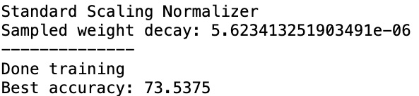
Figure 8.11 – Accuracy results
As you can see, we are getting 73% accuracy on the logistic regression model.
The accuracy reflects the features that were learned in a completely unsupervised manner and without any labels. We have compared those learned features to a traditional classifier as if labels were present. And then, by passing a fraction of the labels, we can achieve an accuracy that is comparable to having the labelled dataset. As mentioned previously, with a better training capacity, you can achieve the results mentioned in the original paper, that is, 95% accuracy with just 1% of the labels.
You are strongly encouraged to repeat the evaluation steps by varying the number of labeled training sets and comparing that with the full training of all labels. That would help demonstrate the immense power of Self-Supervised Learning.
Next steps
While we have only built a supervised classifier to use the features learned from the SimCLR model, the SimCLR model utility does not have to be limited to it. You can use representations learned from unlabelled images in various other fashions:
- You can compare the features learned by using a dimensionality reduction technique. By using Principal Component Analysis (PCA), you can map the features to a higher dimensional space and compare them.
- You can also use some anomaly detection methods, such as One-Class SVM, to find outliers in the images.
Apart from these, you can also try tweaking the SimCLR architecture code and building new models. Here are some ways to tweak the architecture:
- You can try another supervised classifier to fine-tune, such as MLP, and compare the results.
- Try the model training with other encoder architectures, such as ResNet-18, ResNet-152, or VGG, and see whether that gives a better representation of the features.
- You can also try training from scratch, especially if you are using it for another dataset. Finding a set of images that is unlabelled should not be a challenge. You can always use ImageNet labels for some similar classes as your validation labels for your fine-tuned evaluation classifier, or manually label a small number and see the results.
- Currently, the SimCLR architecture uses the NTXent loss function. If you are feeling confident, you could play with a different loss function.
- Trying some loss functions from Generative Adversarial Networks (GANs) to mix and match GANs with self-supervised representation can be an exciting research project.
Finally, don't forget that SimCLR is just one of the many architectures for contrastive learning. PyTorch Lightning also has built-in support for other architectures, such as CPC, SWAV, and BYOL. You should try them out, too, and compare the results with SimCLR as well.
Summary
Most of the image datasets that exist in nature or industry are unlabeled image datasets. Think of X-ray images generated by diagnostic labs, or MRI or dental scans, and many more. Pictures generated on Amazon reviews or images from Google Street View or e-commerce websites like EBay are also mostly unlabelled; also a large proportion of Facebook, Instagram, or WhatsApp images are never tagged and are therefore unlabelled as well. A lot of these image datasets remain unused with untapped potential due to current modelling techniques requiring large amounts of manually labelled sets. Removing the need for large, labelled datasets and expanding the realm of what is possible is Self-Supervised Learning.
We have seen in this chapter how PyTorch Lightning can be used to quickly create Self-Supervised Learning models such as contrastive learning. In fact, PyTorch Lightning is the first framework to provide out-of-the-box support for many Self-Supervised Learning models. We implemented a SimCLR architecture using PyTorch Lightning and, using built-in functionalities, easily created a model that would have taken a lot of effort on TensorFlow or PyTorch. We have also seen that the model performs quite well with a limited number of labels. With as little as 1% of the dataset labelled, we achieved results that are comparable to using a 100% labeled set. We can distinguish the unlabelled images from each other purely by learning their representations. This representation learning method enables the additional methods to identify anomalous images in the set or automatically cluster the images together. Self-Supervised Learning methods such as SimCLR are currently considered to be among the most advanced methods in Deep Learning.
So far, we have seen all the popular architectures in Deep Learning, starting with CNNs, moving on to GANs, and then to Semi-Supervised Learning, and finally to Self-Supervised Learning. We will now shift our focus from training the models to deploying them. In the next chapter, we will see how we can take models to production and familiarize ourselves with the techniques to deploy and score models.